Design and testing of a DDG51 destroyer model

Design and Testing of a DDG51 Destroyer Model

by

Muriel Claire Thomas

Ingenieur dipl6mee de 'Ecole Polytechnique (July 1999)

Submitted to the Ocean Engineering Department

in partial fulfillment of the requirements for the degree of

Master of Science in Naval Architecture and Marine Engineering

at the

MASSACHUSETTS INSTITUTE OF TECHNOLOGY

February 2002

@

Massachusetts Institute of Technology 2002. All rights reserved.

Author ...

Ocean Engineering Department

January 18, 2002

Certified by...

I

Michael S. Triantafyllou

Professor of Ocean Engineering

Thesis Supervisor

A ccepted by ... ...

...

...

Professor Henrik Schmidt

Chairman, Departmental Committee on Graduate Studies,

MAS9ACHUSETSIu " OF TECHNOLOGY

APR 2 6 2002

Department of Ocean Engineering

MIT Libraries

Document Services

DISCLAIMER OF QUALITY

Due to the condition of the

original material, there are unavoidable

flaws in this reproduction. We have made every effort possible to

provide you with the best copy available. If you are dissatisfied with

this product and find it unusable, please contact Document Services as

soon as possible.

Thank you.

The images contained in this document are of

the best quality available.

Design and Testing of a DDG51 Destroyer Model

by

Muriel Claire Thomas

Submitted to the Ocean Engineering Department on January 18, 2002, in partial fulfillment of the

requirements for the degree of

Master of Science in Naval Architecture and Marine Engineering

Abstract

Building an accurately scaled model of a real ship still remains a very important step in ship design. Even though the 3-D computer models are more and more precise and reliable, tests on models give such precious information on the ship behavior that they cannot be avoided yet. The most common test performed with scale models are towing and turning tests, where a scale model of the hull is attached to a carriage in a towing tank (linear or circular). In order to do more complex tests, for example maneuverability tests, a more elaborate model of the ship has to be built. The model needs to have the following characteristics: the model needs to be autonomous, in the sense that it has no physical link with the operator (data are sent wirelessly), and the boat needs to be equipped with sensors to record all the model boat parameters. This implies that not only does the boat need to have its own power supply, but it also needs to have the capacity to receive and execute the commands sent by the operator and finally to store the sensors data or to send them back directly to the operator. The rapid development of computer technologies makes it affordable to equip a model boat with a computer such as a PC104 to execute all the tasks required in real-time. The model boat is controlled remotely by a laptop sending wirelessly the commands entered by the operator to the boat on-board computer. The main motors RPM and rudder position are close-loop controlled. To limit data exchange and the risk of breaking the connection, the sensors data are stored on board and not sent real-time to the operator. Three type of sensors are used: an inertial unit giving x, y and z accelerations and roll, pitch and yaw rotation rates, a magnetometer giving the heading of the boat and a differential GPS giving position, heading, velocity and much more.

Several levels can be distinguished in building a remote control boat. The first three can be defined as follows: first controlling the velocity and the rudder position, which allows driving the boat around completely remotely. The second step is to control the heading of the boat which gives more possibilities in the type of tests that can be performed on the boat. The third step would be to control the position of the boat. A further step would include for example surge control.

At the beginning of this work, the first step in remote control was already achieved, the computer system and data logging system were already operational. The goal was to achieve the second step in remote control and do extensive testing on the model boat. The third step of remote control, closely linked to the second step, was initiated.

Thesis Supervisor: Michael S. Triantafyllou Title: Professor of Ocean Engineering

Acknowledgments

All the work I present here would not have been possible without the help of many people I

would like to thank here.

First, I would like to thank my thesis supervisor Michael S. Triantafyllou and principal research engineer Franz S. Hover for offering me to work on this exciting project and for helping me with the many problems I encountered during my research.

Of course, I cannot forget my friends and fellow students of the towing tank: Craig Martin

and Joshua Davis, who both graduated before me, David Beal, Anna Michel, Stephen Licht, Victor Polidoro and Karl-Magnus McLetchie for their advice and support. Special thanks go to Martin Stoffel who helped me from Switzerland and Matt Greytak, who worked as a UROP on this project during the fall semester; their help was extremely valuable to me.

I would also like to thank all the people who made the testing of the boat possible: Fran Charles manager of the MIT Sailing Pavilion, Rich Axtell manager of the Hanscom Swimming

Pool, Tom Consi from the OE department, Brian Callahan manager of the MIT swimming pool

and finally Rick Meyer and BAE Ocean Systems for letting us use their open water test facility in Braintree.

I am also grateful to the people of the Diligation Geinrale pour l'Armement, Direction des Constructions Navales and Ecole Nationale Sup rieure de Techniques Avancees for giving me

the great opportunity to come and study here at MIT.

Finally, I would like to dearly thank my fiance Geoffroy for his loving and helpful support throughout my studies at MIT.

Contents

1 INTRODUCTION

1.1 Background and Previous Work . . . .

1.1.1 DDG51 Model Hull Background . . . .

1.1.2 M otivations . . . . 1.2 Thesis Objectives . . . .

1.3 Thesis Contribution . . . .

1.4 Thesis Outline . . . . 2 SENSORS

2.1 DMU (Accelerometers and Gyros) . . . .

2.1.1 Coordinate System . . . . 2.1.2 Importance of the Position of the DMU . . . . .

2.1.3 DM U Data . . . .

2.1.4 Building a Test Bench . . . . 2.1.5 Processing the Data . . . .

2.1.6 Obtaining the Boat Data from the DMU Data .

2.1.7 Boat Path . . . .

2.2 M agnetometer . . . . 2.2.1 Specifications . . . . 2.2.2 Position of the Magnetometer in the Boat . . . 2.2.3 Data Processing . . . .

2.3 D G P S . . . .

2.3.1 Data Transmitted . . . . 2.3.2 Data Processing . . . .

2.4 Data Processing Program . . . .

2.5 Sum m ary . . . .

3 DESIGN OF A HEADING CONTROLLER

3.1 Ship Steering Equations . . . .

3.1.1 Non-Linear Ship Steering Equations . . . .

3.1.2 Linear Ship Steering Equations . . . .

3.2 The Models of Nomoto . . . .

3.2.1 Nomoto's Second Order Model . . . .

3.2.2 Nomoto's First Order Model . . . .

3.3 Hydrodynamic Coefficients . . . . 3.3.1 Nomoto's Coefficients from SBT . . . .

3.3.2 Nomoto's Coefficients from Model Experiments .

13 13 13 14 14 15 15 18 18 18 19 20 20 23 25 25 26 26 26 27 28 28 28 30 33 34 34 34 34 . 36 36 38 38 . . 39 41

3.4 Designing the Heading Controller . . . . 3.4.1 Choice of the Type of Controller . . . . 3.4.2 Controller Equations and Parameters . . . . 3.5 Adapting the Controller . . . .

3.5.1 Gain Scheduling . . . . 3.5.2 The Parameters Which Influence the Controller . . . .

3.5.3 Study of the Influence of the Forward Velocity . . . . 3.5.4 Finding the Parameters Ko and To . . . .

3.6 Discrete Controller . . . .

3.6.1 Why Discretize the Controller? . . . . 3.6.2 Equations for the Discrete Controller . . . .

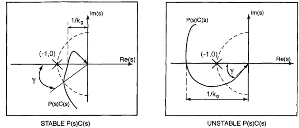
3.7 Evaluating the Controller Robustness . . . . 3.7.1 Measures of the Robustness . . . .

3.7.2 Implementing Rudder Limitations . . . .

3.7.3 Analysis of the Matlab Program for Testing the Controller

3.8 Sum m ary . . . .

4 IMPLEMENTATION OF THE HEADING CONTROLLER

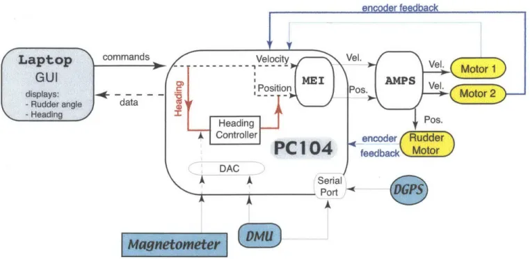
4.1 Boat Operating System . . . . 4.1.1 System Overview . . . . 4.1.2 System Components Description . . . . 4.2 Controller Specificities . . . . 4.2.1 Working requirements . . . . 4.2.2 Implementation . . . . 4.3 Sum m ary . . . . 5 TRACK KEEPING 5.1 Introduction . . . .

5.2 Kinematics for track keeping . . . . 5.3 Guidance by Line of Sight . . . . 5.4 Matlab Program for Track Keeping system

5.4.1 Overall Structure . . . . 5.4.2 Analyzis of the program . . . .

5.5 Implementing the Position Controller . . . . 5.6 Summary . . . .

6 TESTING THE BOAT

6.1 Testing Locations . . . .

6.2 Preparing the Boat for Outdoors Testing .

6.3 Presentation of the tests . . . .

6.3.1 Velocity Tests . . . .

6.3.2 Simple Turning Tests . . . . 6.3.3 Dieudonne spiral maneuver . . . .

6.3.4 ZigZag Maneuver . . . .

6.3.5 Circle Maneuver

6.3.6 Evaluating the Tactical Diameter Before Testing .

42 42 44 45 45 46 47 48 50 50 51 51 52 53 53 55 56 56 56 57 68 68 68 70 71 71 71 72 73 73 73 76 76 77 77 78 78 79 79 79 81 83 84

. . . .

7 RESULTS AND ANALYSIS 7.1 Velocity Tests ... 7.2 Turning Tests ... 7.2.1 Tests Description ... 7.2.2 Values of Ko and To . . . . . . . . . . 7.2.3 Analysis of a Turn ...

7.3 Results of the Circle Maneuver Tests .

7.3.1 Description of the Tests . . . .

7.3.2 Analysis of The Tests . . . . 7.4 Summary . . . .

8 CONCLUSION

8.1 Thesis Summary . . . .

8.2 Conclusions . . . .

8.3 Recommendation for Future Work . . . . .

A DDG51 Characteristics B SHIP MODEL PAYLOAD

C DMU TESTING

C.1 Test Bench . . . . C.2 Other Tests . . . .

D SHIP PATH USING DMU DATA

D .1 M ethod . . . .

D.2 Matrices Relations ...

E SLENDER BODY THEORY

E.1 Fluid force -Y hydrodynamic coefficients

E.1.1 Reference Frame ...

E.1.2 Elementary Fluid force ...

E.1.3 Total Fluid force ...

E.1.4 Y Hydrodynamic Coefficients . ...

E.2 Fluid Moment ...

E.2.1 Elementary Fluid moment ...

E.2.2 Total Fluid Force ...

E.2.3 Hydrodynamic Coefficients...

E.3 Computing SBT hydrodynamic coefficients E.3.1 Elementary added mass ...

E.3.2 "Rectangular Platform" estimation

E.4 Other ways to compute the hydrodynamic coefficients . E.4.1 Semi-empirical Methods and Regression Analysis E.4.2 Fossen's approximations . . . .

F SCALING & NON-DIMENSIONALIZATION

F.1 Scaling process ... F.2 Non-Dimensionalization . . . . 131 . . . 131 . . . 133 86 86 87 87 87 88 95 95 97 .103 105 .105 .106 .107 109 112 113 .113 .116 117 .117 .118 123 .123 .123 .124 .125 .126 .126 .126 .127 .127 .128 .128 .128 .129 .129 .130

.

G YAW RATE GRAPHS

Hanscom Swimming Pool- Feb. 2001 134

H FIFO'S AND THREADS 137

H.1 FIFO'S ... ... 137

H .2 T hreads . . . .. 138

H.2.1 Laptop Threads ... ... 138

H.2.2 PC104 Threads ... 138

I YAW RATE GRAPHS

MIT Alumni Swimming Pool, Dec. 2001 140

J GLOBAL RESULTS

MIT Alumni Pool - Dec. 2001 Tests 151

List of Figures

DMU reference frame . . . .

Boat equipment layout . . . . Body frame fixed with the boat . . . . Test Bench for the DMU. . . . . Reference frame of Magnetometer . . . . Matlab Graphical User Interface for data processing . . . . Reference frames and motion parameters . . . . Rudder Position . . . .

Comparison between the first and second order Nomoto models Ship Model Experience - Hanscom Swimming Pool . . . . Comparison between the first and second order Nomoto models Heading controller . . . . Gain scheduling controller . . . . Difference between a continuous and a digital controller . . . .

Sampling and Holding Process . . . .

Gain and Phase Margin Definitions . . . . 4-1 Boat Global Operating System . . . . 4-2 Ship model Graphical User Interface (on Laptop) . . . . .

4-3 Ship model GUI from [17] . . . .

4-4 PC104 software diagram . . . . 4-5 Laptop software diagram . . . .

5-1 Coupled position and heading controller . . . .

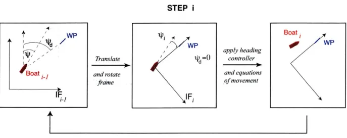
5-2 Step of the autopilot Matlab program . . . .

5-3 Result of the Matlab autopilot program . . . .

6-1 Path during a Dieudonne Spiral Maneuver (Stable Ship) .

6-2 Relation between rudder angle and yaw turning rate . . . 6-3 Overshoot and zigzag maneuver . . . . 6-4 Turning Test . . . . 7-1 Velocity Tests at the MIT pool and Towing Tank . . . . .

7-2 Velocities and Acceleration during a turn . . . .

7-3 X, Y and Z accelerations measured by the DMU . . . . .

7-4 Stabilized Pitch and Roll angles measured by the DMU . 7-5 Roll, Pitch and Yaw Rotation rates measured by the DMU

. 18 . . 19 . . 20 . . 21 26 . 31 . . . . 35 . . . 35 . . . 41 . . . 42 . . . 43 . . . 44 . . . 46 . . . . 50 . . . . 51 . . . . 52 . . . . 5 7 . . . 6 1 . . . 6 1 . . . . 6 7 . . . 6 8 . . . . 7 3 . . . 7 4 . . . . 7 5 . . . 8 0 . . . 8 0 . . . 8 2 . . . 8 3 . . . 8 7 . . . 9 1 . . . 9 3 . . . 9 3 . . . . 9 5

7-7 Comparison between the magnetometer heading and the yaw rate integration

C-1

C-2 C-3

C-4

Testing Configuration 1 for DMU Test Bench . . . . Testing Configuration 2 for DMU Test Bench . . . . Expected Measurement from the DMU . . . . Experimental Data from DMU . . . .

D-1 Method to obtain the ship path using the DMU data . . . . D-2 Comparison between the positions given by the GPS and the DMU method

. . . 113 114 . . 114 . . . 115 . . . 117 . . .121

E-1 Coordinate Systems for SBT . . . . E-2 Ship Approximation . . . . G-1 Experiments in Hanscom Pool - 1/2 . . . . G-2 Experiments in Hanscom Pool - 2/2 . . . . Yaw rotation rates curve fitting for different experiments (1/6) Yaw rotation rates curve fitting for different experiments(2/6) Yaw rotation rates curve fitting for different experiments(3/6) Yaw rotation rates curve fitting for different experiments(4/6) Yaw rotation rates curve fitting for different experiments(5/6) Yaw rotation rates curve fitting for full turn experiments(6/6) . . . 124 . . . 128 . . . 135 . . . 136 . . . 141 . . . 143 . . . 145 . . . 147 . . . 149 . . . 149

J-1 Turning Tests at 200 RPM and 30 deg. J-2 Turning Tests at 200 RPM and 35 deg. J-3 Turning Tests at 300 RPM and 10 deg. J-4 Turning Tests at 300 RPM and 20 deg. J-5 Turning Tests at 300 RPM and 30 deg. J-6 Turning Tests at 400 RPM and 10 deg. J-7 Turning Tests at 400 RPM and 20 deg. J-8 Turning Tests at 400 RPM and 30 deg. J-9 Turning Tests at 400 RPM and 35 deg. J-10 Turning Tests at 500 RPM and 10 deg. J-11 Turning Tests at 500 RPM and 20 deg. J-12 Turning Tests at 500 RPM and 30 deg. J-13 Turning Tests at 500 RPM and 35 deg. J-14 Turning Tests at 600 RPM and 10 deg. J-15 Turning Tests at 600 RPM and 20 deg. J-16 Turning Tests at 600 RPM and 35 deg. J-17 Turning Tests at 500 RPM and 20 deg. J-18 Turning Tests at 500 RPM and 30 deg. J-19 Turning Tests at 500 RPM and 35 deg. J-20 Turning Tests at 600 RPM and 10 deg. J-21 Turning Tests at 600 RPM and 20 deg. J-22 Turning Tests at 600 RPM and 35 deg. J-23 Turning Tests at 500 RPM and 20 deg. J-24 Turning Tests at 500 RPM and 30 deg. J-25 Turning Tests at 500 RPM and 35 deg. J-26 Turning Tests at 600 RPM and 10 deg. - Alumni Pool - Alumni Pool - Alumni Pool - Alumni Pool - Alumni Pool - Alumni Pool - Alumni Pool - Alumni Pool - Alumni Pool - Alumni Pool - Alumni Pool - Alumni Pool - Alumni Pool - Alumni Pool - Alumni Pool - Alumni Pool - Alumni Pool - Alumni Pool - Alumni Pool - Alumni Pool - Alumni Pool - Alumni Pool - Alumni Pool - Alumni Pool -Alumni Pool -Alumni Pool . . . 153 . . . 155 . . . 157 . . . 159 . . . 16 1 . . . 163 . . . 165 . . . 167 . . . 169 . . . 17 1 . . . 173 . . . 175 . . . 177 . . . 179 . . . 18 1 . . . 183 . . . 185 . . . 187 . . . 189 . . . 19 1 . . . 193 . . . 195 . . . 197 . . . 199 . . . 20 1 . . . 20 3 I-1 1-2 1-3 I-4 I-5 1-6 . . 97

Turning Tests at 600 RPM and 20 deg. Turning Tests at 600 RPM and 35 deg. Turning Tests at 700 RPM and 10 deg. Turning Tests at 700 RPM and 20 deg. Turning Tests at 700 RPM and 30 deg. Turning Tests at 700 RPM and 35 deg. Turning Tests at 800 RPM and 10 deg. Turning Tests at 800 RPM and 20 deg. Turning Tests at 800 RPM and 30 deg. Turning Tests at 800 RPM and 35 deg.

-Alumni Pool - Alumni Pool - Alumni Pool - Alumni Pool - Alumni Pool - Alumni Pool - Alumni Pool - Alumni Pool - Alumni Pool - Alumni Pool . . . 205 . . . 207 . . . 209 . . . 211 . . . 213 . . . 215 . . . 217 . . . 219 . . . 221 . . . 223

K-1 GPS position data - BAE Quarry (1/2) ... K-2 GPS position data - BAE Quarry (2/2) ... K-3 Circle Maneuver tests at 300 RPM and 10 deg. - BAE Quarry K-4 Circle Maneuver tests at 300 RPM and -20 deg. - BAE Quarry K-5 Circle Maneuver tests at 300 RPM and -30 deg. - BAE Quarry K-6 Circle Maneuver tests at 500 RPM and -10 deg. - BAE Quarry K-7 Circle Maneuver tests at 500 RPM and -20 deg. - BAE Quarry K-8 Circle Maneuver tests at 500 RPM and -30 deg. - BAE Quarry K-9 Circle Maneuver tests at 700 RPM and -10 deg. - BAE Quarry K-10 Circle Maneuver tests at 700 RPM and -20 deg. - BAE Quarry K-11 Circle Maneuver tests at 700 RPM and -30 deg. - BAE Quarry . . . 227 . . . 229 . . . 231 . . . 233 . . . 235 . . . 237 . . . 239 . . . 241 . . . 243 . . . 245 . . . 247 J-27 J-28 J-29 J-30 J-31 J-32 J-33 J-34 J-35 J-36

List of Tables

1.1 Principal characteristics of the DDG51 . . . . 2.1 Position of the DMU compared to the center of gravity of the boat . . . . 2.2 DMU data versus connector pin . . . . 2.3 Accelerometer Calibration Data . . . . 2.4 Gyro Calibration Data . . . .

2.5 Recommended Minimum Specific Data from the DGPS . . . . 3.1 Values of Dimensional and ND Hydrodynamic Parameters of the Scaled Boat . .

17 20 21 24 24 29 40

Experimental evaluation of the K ans T coefficients . . . 43

Non-dimensional values of K and T for different models . . . 48

RPM - Forward Velocity Correspondence . . . . 49

Nomoto's constants from experiments . . . 49

Rudder rotation rate limitations . . . 54

Ship Model Controller Robustness Characteristics . . . . 54

Ship Model Controller Close-Loop Poles . . . 55

Shell scripts for data transmission . . . 65

Laptop Fifo's list and description . . . 65

PC104 Fifo's list and description . . . 66

Turning radius according to [14] . . . . Turning radius according using hydrodynamic coefficients . . . RPM - Forward Velocity Correspondence . . . . Experimental evaluation of the K ans T coefficients . . . . Circle Maneuver Macros . . . . Tactical and steady turning diameters and steady yaw rates for GPS Velocity and Variation in sway velocity for the GPS . . . List and Heel at rest, Steady Roll angle during a turn . . . . . GPS lag and drift angle . . . . 85 85 . . . . circle maneuvers 88 89 97 98 100 . . . 103 . . . 104

A.1 Real DDG51 Parameters . . . 109

A.2 Propeller and LM2500 Characteristics . . . .. 110

B.1 Weight and position fo the equipment . . . 112

C.1 Macro Description . . . 113

H.1 FIFO list and data structure . . . 137

3.2 3.3 3.4 3.5 3.6 3.7 3.8 4.1 4.2 4.3 6.1 6.2 7.1 7.2 7.3 7.4 7.5 7.6 7.7

Chapter 1

INTRODUCTION

1.1

Background and Previous Work

1.1.1

DDG51 Model Hull Background

The hull used for this project is a 1:47 scaled model of a US Navy Arleigh Burke Class De-stroyer (DDG51). The dimensions of the real boat are given in Appendix A and the comparison between the model and the real boat is shown in Table (1.1). The hull was built around ten years ago at the David Taylor Model Basin. The hull is made of fiberglass and few pieces of wood at the bow, the stern and on the rim; it has a sonar dome shape at the bow. When given to the MIT Towing Tank, it was a bare hull and basically made only for towing tests. However, it was used for quite different experiments as described below.

The first study carried on this hull was a DPIV (Digital Particle Image Velocimetry) study on the hull. Then, the hull was used for the foilboat project (cf. [2]), which was quite successful.

A third study led to modify the hull in order to transform it into a remote control boat.

Two shafts and five-blade propellers were added, and two rudders were attached at the stern. The hull was also equipped with two half horse power DC brush motors to drive the two shafts and propellers and a small motor to activate the rudder. An on board computer was also added along with sensors (a six-axis inertial unit and a magnetometer). However, only a few tests were done at the towing tank and the model was never fully remotely controlled (cf. [22]).

Great progress was made on the ship model system by Stoffel (cf. [17]). Actually, Stoffel redesigned the whole operating system: the on board computer was changed and operated

under Linux and a relatively robust remote control program was built along with a data logging system. All the programs were written either in C or C++. A Differential GPS was added to the two other sensors. The boat was successfully tested at the MIT Towing Tank and at Hanscom Swimming pool.

1.1.2 Motivations

The naval ships of the next generation are being considered as having a reduced manning, so more and more control systems have to be developed: controlling the surge, sway, yaw motions, ship tracking, heading, fuel consumption optimization and engine propeller dynamics are a few examples. Ship motions and engine dynamics being multivariable systems, a MIMO (Multiple Input Multiple Output) study should be considered.// Even if a SISO (Single Input Single Output) PID controller is a great simplification compared to the real control case, it can serve as a solid ground to develop more complex controllers afterwards.

Then, considering the limitations and capabilities of actual simulation and design techniques, experimentation on ship models is still needed. Maneuvering of naval combatants is almost com-pletely neglected in the design process and usually the maneuvering capabilities are accepted as determined by the full-scale sea trials after the ship has been built. Consequently, an accurately scaled ship model remotely operated and equipped with controllers for the parameters men-tioned above could help to evaluate at a relatively low cost the maneuvering capabilities of the real ship. This could lead to some modifications in order to improve the real boat performance before the boat has actually been built.

1.2

Thesis Objectives

The main thesis objective is to design and implement a simple PID SISO heading controller for the model boat and test it successfully along with doing some other testing on the boat to characterize its maneuvering capabilities.

To achieve the thesis main goal, it was necessary to subdivide it into several specific objectives:

" acquire a full understanding of the system designed in [17],

" design a simple model of the boat yaw-sway behavior from available data and

experi-ments,

1.2 Thesis Objectives

INTRODUCTION 1.3 Thesis Contribution

" optimizing the preparation and time necessary for testing the boat,

" designing a sequence of tests that would fully reflect the boat maneuvering capabilities, " interpreting the results in order to refine the yaw-sway model and evaluate the

maneu-vering capabilities of the model boat.

In fact, the initial global goal of the thesis was broader and included building a surge controller in order to replicate the dynamics of the two LM2500 gas turbine of the real ship. This could not be achieved due to a lack of time, however the same method as the one used to design the heading controller can be used to design the surge controller.

1.3

Thesis Contribution

The thesis presents many processes that are part of the heading controller design and im-plementation and introduces the required concepts and procedures to build and implement the position controller. The thesis also provides several other main contributions:

" Keep the boat in a good working state and improve the boat layout and the reliability

of the boat system,

" document thoroughly the boat operating system, the way to prepare the boat for testing,

the way to operate it during the test and the way to post-process data. Organized documentation is really essential for all the work done in this thesis and in [17] to be used efficiently.

" develop simple and efficient Graphical User Interfaces (GUI) for the boat remote control

system and data processing,

" and finally provide data on the ship model that can be used for further maneuvering

studies.

1.4

Thesis Outline

The thesis organization follows the chronology of the work done. The five major steps of the work accomplished are each described in a chapter:

" Chapter 2: the subject of this chapter is the three sensors which equip the boat:

the inertial unit, the magnetometer and the DGPS. The main goal of the chapter is to describe data processing for each of the sensors along with the overall post-processing Matlab program. Accurate data processing is crucial to be able to interpret the results of the tests described in Chapter 6.

" Chapter 3: this chapter is mainly concerned with the design of a robust heading controller for the ship model. The biggest concern of the chapter is to find an accurate

plant model for the boat. The first order Nomoto model is used and the chapter presents several possible ways to obtain the parameters of this model. The method to verify the robustness of the controller is also described.

" Chapter 4: the goal of this chapter is to explain the actual boat operating system and

especially the modifications which have been applied to the system designed by Stoffel. The GUI, the remote control program and the implementation of the heading controller are described in detail.

" Chapter 5: this chapter gives indications on how to use the heading controller to build

a track controller.

" Chapter 6: its topic is the ship model testing, which was the ultimate goal of the project.

the choice of the testing locations is analyzed along with the necessary preparation before testing the boat. Finally the tests performed on the boat are thoroughly described.

" Chapter 7: all the results and data processing of the tests listed in Chapter 6 are

presented along with a conclusion.

1.4 Thesis Outline

Characteristics Real Ship Ship Model' Length (LOA2) 149.98 m 3.25 m Length (LBP3) 142.04 m 3.15 m Beam 17.98 m 44 cm Draft 6.1 m 15.2 cm Displacement 8340 T 864 kg Waterplane area 2029.23 m2 1 m2 LCG 5 0.85 m after midships 0.05 m

Block Coefficient 0.522 idem

Prismatic coefficient 0.615 idem

Top speed 32 knots (14m/s) 4.67 knots (2.4 m/s)

Sustained speed 20 knots (10.3 m/s) 2.9 knots (1.5 m/s)

Prop. diameter 5.18 m 10.8 cm

Number of propellers 2 2

Number of blade on one prop 5 (CP6) 5 (fixed pitch)

Table 1.1: Principal characteristics of the DDG51

'for LBP, LOA, B and D, measurements were taken on the model hull itself

2

Length Over All 3

Length Between Perpendicular 4

Estimated total weight

5

Longitudinal center of Gravity

Chapter 2

SENSORS

The boat uses the three following sensors:

" Three axis accelerometers and three axis gyros: DMU VGX from Crossbow (www.xbow.com).

In the rest of the thesis, it will be referenced to as DMU.

" Magnetometer: model 113 from Crossbow,

" Differential GPS (DGPS): DGPS 53 from Garmin (www.garmin.com).

In the following, data processing is described sensor by sensor.

2.1

DMU (Accelerometers and Gyros)

2.1.1 Coordinate System

The axis of the DMU are positioned as shown in Figure (2-1). For all the experiments,

I- -Y DMU Zbox

Bow of the boat wires

Z

SENSORS 2.1 DMU (Accelerometers and Gyros)

Propeller

Rudder motor _{Main motor B= 0.44 Magnetometer}

0 PC104

Aiur 22Bo Battery

MlcdoainlhebwDGPS

m ta eof pte Aerial SRudder Rudder motor plate

L =3.25 m

Figure 2-2: Boat equipment layout

due to, the layout of the equipment inside the boat (cf. Figure (2-2)), the wires will always be

placed facing the bow..

2.1.2 Importance of the Position of the DMU

Studying the movements of the boat means working with two coordinate systems:

" the inertial reference frame, which is Earth based. As the range used for testing the

boat is significantly smaller than the Earth dimensions and considering the fact that each test on the boat does not last more--than a few minutes, this frame will be considered

fixed. For the rest of this report, this frame will be referred to as IF (Inertial Frame), " the body fixed frame, which is attached the ship model. This frame is shown on Figure

(2-3). The origin of this frame is positioned at midships, X is pointing at the bow, Y is

pointing port and Z is pointing down. This is the frame used in references [3] and [8]. One obvious reason for positioning this frame at midships and not at the center of gravity (Cog) is because the center of gravity of the boat depends on the loading of the ship and thus can change over time. For the rest of this report, this frame will be referred to as

BF (Body Frame).

As it will be shown later, knowing the movement of the boat in the BF is crucial to the analysis of the boat behavior. However, the DMU gives the values of the accelerations and the

SENSORS

midships

x

Y

Figure 2-3: Body frame fixed with the boat Item Position of the Center

of Gravity wrt midships Total Payload -0.058 m

Hull + Payload -0.025 m DMU center -0.0475 m

Table 2.1: Position of the DMU compared to the center of gravity of the boat

to the position of the boat should be taken into account.

To determine the position of both the DMU and the Cog with respect to midships, a payload sheet was filled with all the weight and position data available for all the pieces of equipment inside the boat. The complete payload sheet is presented in Appendix B. A brief summary is presented in Table (2.1). In this table, the position of the center of gravity of the boat is only an estimation, but DMU and Cog are very close to each other and also close to midships. The center of the DMU is taken as the center of the sensor black box. Using those results, it was supposed for all data processing that the boat Cog , the DMU frame center and boat midships were merged.

2.1.3 DMU Data

The DMU has three different working modes (cf. [19]). The mode that was used is the so called angle mode which allows the gyro to output the stabilized pitch and roll angles along with the three angular rates and the three accelerations. The data available in the angle mode are given in table Table (2.2).

2.1.4 Building a Test Bench

Building a small testing facility for the DML-was a necessary step in understanding the way

SENSORS 2.1 DMU (Accelerometers and Gyros)

Pin Signal

5 X-axis acceleration (Analog Voltage)

6 Y-axis acceleration (Analog Voltage)

7 Z-axis acceleration (Analog Voltage)

8 Roll rate analog voltage

9 Pitch rate analog voltage

10 Yaw rate analog voltage

12 Roll analog voltage (stabilized Roll voltage)

13 Pitch analog voltage (stabilized Pitch voltage) Table 2.2: DMU data versus connector pin

,Figure 2-4: Test Bench for the DMU

shown on Figure (2-4) . One of the main motor of the DDG51 ship model was coupled to an axis on which a wooden plate was attached. The DMU was then attached on this plate and could thus be moved.

The motions of the motor were controlled using the remote control program of the DDG51 design by Stoffel (cf [17]). More precisely, the macro mode of this remote control program was used. This mode allows for each motion to set the RPM and the duration of the motion. The data from the DMU were recorded using the data logging feature of the remote control program. The main asset of such a testing device is that the rotation rates and accelerations are known. Thus, those values can be compared with the DMU logged data.

The test bench allowed to find two mistakes in the previous use of the DMU:

e the wrong working mode was used in [17], which led to having other measurements of the

x and y accelerations instead of the stabilized pitch and roll angles on pins 12 and 13 (cf.

2.1 DMU (Accelerometers and Gyros) SENSORS

2.1 DMU (Accelerometers and Gyros)

* the gravity components is opposite to the expected values on the x and y axis but the measured accelerations other than gravity are accurate. On the z axis the gravity compo-nent is measured accurately but the accelerations other than gravity are opposite to the real values.

Some of the tests performed with the DMU test bench are presented in Appendix C.

2.1.5 Processing the Data

All the data conversions are detailed in the DMU manual, reference [19]. Here are only mentioned the conversions used in the data processing programs.

The data from the DMU are collected via the Data Acquisition Card (model DAS16jr/12 from Computer Boards) as 12 bits numbers between 0 and 4096. The DAC has 16 analog input channels which can be sampled at a maximum rate of 10kHz. The analog output voltage of the DMU being between +5V and -5V, Equation (2.1) is used to convert the data of the DAC back into volts:

analog data - 2048

Vout[V] outtj4096 -9 10 (2.1)

where V0ut is the value in volts of the analog output voltage.

Then, each of the voltages has to be converted into the engineering units of the data they represent (M/s2 for accelerations, deg/s for rotation rates and deg for angles).

Acceleration Data

The analog outputs for acceleration are "raw data" from the DMU, so both offsets and sensitivity factors are needed to convert the voltage into engineering units. So for the accel-erations (pins 5, 6 and 7 of the DMU connector), Equation (2.2) is used for the conversion to

m/s2:

accel[m/s2

] = (Vut [V] - offset) - sensitivity - 9.81 (2.2) where the offsets and sensitivities have specific values for each of the three axis. The default values of the offsets and sensitivities are specific to each DMU and given in the specification sheet of the unit. For acceleration data, the specifications of the DMU used in the boat are mentioned in Table (2.3).

Rotation Rate Data

For the rotation rates (roll, pitch and yaw rates on pins 8, 9 and 10), the analog outputs are not the raw values from the sensors, they already have been processed by an internal converter. So the offsets of the axis are not needed and Equation (2.3) is used to convert the volts V0st

into */s:

V

ut [V ]

rate ['/s] = AR - 1.5.

4-09

[VI

4.096 [V]

where AR is the angular rate range of the sensor which is given in Table (2.4) for each axis of the gyro. The offsets and sensitivities are also given, even if they are not directly used here.

Stabilized Angles

As for the stabilized angles (pitch and roll angles), Equation (2.4) is the formula used to convert the analog data Vut into degrees:

angle [0] = 900 -

Vu [V]

4.096[V]

Axis Null Offset Sensitivity Range

(V)

(G/V)

(G)

X 2.570 1.007 2.000

Y 2.482 0.990 2.000

Z 2.480 1.009 2.000

Table 2.3: Accelerometer Calibration Data

Axis Null Offset Sensitivity Range

(V)

(deg/sec/V)

(deg/sec)

X

2.522

73.109

150.000

Y

2.513

63.598

150.000

Z

2.517

60.905

150.000

Table 2.4: Gyro Calibration Data

Then, before processing the data, it has to be noted that the DMU does not internally

correct for gravity. Consequently, the gravity has to be removed from the x, y and z

SENSORS

erations. To do so, the vector ' has to be projected on the axes of the DMU frame and each of its component then subtracted from the initial x, y and z accelerations.

2.1.6 Obtaining the Boat Data from the DMU Data

In have

order to obtain the boat parameters from the DMU parameters, three processing steps to be implemented:

1. modify the DMU data according to Section 2.1.4,

2. remove the gravity from the x and y axis using the stabilized pitch and gravity vector projected on the boat axes and noted ' is:

0 cos(q$) - sin($)

01

roll angles. The

cos(4) 0 - sin(b)

Co = 0 1 0

sin(#) 0 cos (0)

_j

(2.5)

3. since the position of the DMU frame compared to the body fixed frame has to be taken

into account, the DMU data have to be modified through the use of a rotation matrix. The Boat frame is obtained by a rotation of 7Tr around the z vertical axis, which is the

same for both frame. If ADMU and Aboat are respectively the acceleration vectors in the

DMU frame and in the boat frame, and if RDMU and Rboat are the rotation rate vectors:

-1 0 01 0 -1

0

The yaw rate and the z accelerations do not need to be changed.

2.1.7 Boat Path

It is possible to use the DMU data to obtain the path followed by the boat. The method is described in detail in Appendix D. It uses integration of the DMU data and the Euler angles. However, this method does not lead to good results, the integration of the DMU data not being precise enough. Some comparisons between the GPS path and the path obtained with DMU

Aboat

[

2.1 DMU (Accelerometers and Gyros)

g-' = C'P -Co -9,)

1

C4 = 0

2.2

Magnetometer

2.2.1

Specifications

The model 113 from Crossbow is designed to measure magnetic fields up to 1 Gauss. The

113 provides 3 analog output voltages proportional to the magnetic field magnitude measured

in three orthogonal directions.

The magnitude of the Earth magnetic field is between 0.6 gauss (at the poles) and 0.3 gauss (at the equator). The gauss is the unit used to measure the Earth magnetic field: 1 gauss = 10-3 testla. The gamma, 1 gamma = 10-6 gauss, is the unit used to measure the disturbances

of the Earth mean magnetic field.

One particularity of this sensor is that its level of noise is very low so that small magnetic signatures can be measured. However, this proves to be a drawback for our application since the DC brush motors used in the model boat generate magnetic field that can disturb the measurement of the magnetometer. Consequently, the sensor had to be placed the farthest away possible from the motors: at the bow of the boat. If the 113 is not disturbed by the magnetic field created the motors or any other exterior source of magnetic perturbation, it can theoretically provide a direction accuracy to better than 0.10.

2.2.2

Position of the Magnetometer in the Boat

It should be noted that the 3 fluxgate sensors of the magnetometer are positioned such that their axes do not form an direct orthogonal frame. The magnetometer is placed as shown on Figure (2-5).

Cables Magnetometer Box

Y

Figure 2-5: Reference frame of Magnetometer

2.2.3 Data Processing

The data from the magnetometer are fairly simple to process since there are no offsets. Only a constant factor is needed to convert the analog data into a engineering data in gauss measuring the intensity of the magnetic field: the sensitivity of the magnetometer is 4V/gauss for all three axes. The formula used to convert analog voltage data to physical data is given in Equation (2.7).

magnetic field [gauss] = analog data - 2048 10[V](2.7)

4096 4[V/gauss]

Then the value of the y axis is reversed to have the components of the magnetic field in the boat frame.

Heading

The magnetometer is mainly used to give the heading of the ship model by measuring the components of the Earth magnetic field. The heading can also be given by the GPS when GPS signals can be received, however GPS heading measurements are obtained only when the boat is moving, whereas the magnetometer can give heading measurements even when the boat is at a standstill.

A first approximation for data processing is to neglect the pitch and roll movements of

the boat. The heading of the boat is the angle between the North and the x axis of the ship model frame and is simply obtained using:

Xmagn > 0 - Boat heading = - arctan Yman) (2.8) \ Xmagn

Xmagn

<

Boat heading

-[arctan

180]

(2.9)

\ Xrmagn /

where heading is computed in degrees, which is more representative than radians, and Xmagn

and Ymagn are the measurements obtained respectively on the x and y axis of the magnetometer. Moreover, heading was chosen to be always given as an angle between 0 and 360 degrees, 0' being North, 900 being East, 1800 being South and 270' being West. So the result of Equations

(??) and (2.9) has to be adjusted for the angle to be in the [0 , 360] degrees interval.

The heading computation could be refine using the stabilized pitch and roll angles of the DMU,

however, since data processing is needed to obtain them, it may slow the heading display on the graphical user interface.

2.3

DGPS

2.3.1 Data Transmitted

The DGPS uses the World Geodetic System 1984 (WGS84) as an earth-centered ref-erence system to localize points. This WGS84 refref-erence system is an earth-centered ellipsoid with the following parameters:

" semi-major axis a = 6,378,137.00 meters

" inverse flattening

}

semi-minor axis).

For more information on the WGS84, the reference [12] can be consulted.

The DGPS has several working modes, each working mode corresponding to a specific output set of data. The set of data used is the Recommended Minimum Specific GPS/TRANSIT

Data (RMC). The set of data transmitted by this mode are given in Table (2.5)

2.3.2 Data Processing

Heading

Heading is obtained using data #8 in Table (2.5). The heading thus obtained is the true

heading (referenced to geographic North). For that data to be compared with the heading

given by the magnetometer (heading referenced to the magnetic North), data #10 (value of the magnetic declination) and #11 (direction of the magnetic declination, West or East) have to be used, using Equation (2.10):

true heading = magnetic heading +(E)

/

The magnetic declination is equal to 15.9 deg. W in Hanscom Air Force Base where the first tests of the ship model were performed, and it is equal to 15 deg. W in the BAE Systems

output sentence:

$GPRMC,<1>,<2>,<3>,<4>,<5>,<6>,<7>,<8>,<9>,<10>,<11>,<12>... ... *hh<CR>< LF >

< 1 > UTC time of position fix, hhmmss format

< 2 > Status, A=Valid position, V=NAV receiver warning

< 3 > Latitude, ddmm.mmmm format (leading zeros will be transmitted)

< 4 > Latitude hemisphere, N or S

< 5 > Longitude, ddmm.mmmm format (leading zeros will be transmitted)

< 6 > Longitude hemisphere, E or W

< 7 > Speed over ground, 000.0 to 999.9 knots (leading zeros will be transmitted

< 8 > Course over ground, 000.0 to 359.9 degrees, true (leading zeros will be transmitted)

< 9 > UTC date of position fix, ddmmyy format

< 10 > Magnetic variation, 000.0 to 180.0 degrees (leading zeros will be transmitted) < 11 > Magnetic variation direction, E or W (westerly variation adds to

the course over ground)

< 12 > _{Mode indicator (only output if NMEA 2.30 active), A=autonomous,} D=differential, E=Estimated, N=data not valid)

Table 2.5: Recommended Minimum Specific Data from the DGPS testing facilities, where the ship model was tested in January 2002.

Position and Trajectory

The position of the boat in the Earth coordinate system is given by data # 3 to 5 in Table

(2.5). The data can be plotted without any processing so that the actual position of the boat

will be given in degrees, minutes and seconds. However, given the small scale of the ship model trajectory, the trajectory can be projected onto an horizontal plane and thus can be plotted on a x-y plot in meters. The origin (0,0) of the plot is taken as the initial position of the boat, x pointing to the East and y pointing to the geographic North.

To obtain the x-y coordinates, the projection of the trajectory on a plane tangent to the initial point is used. Around the initial point, the ellipsoid can be approximated by a sphere of radius equal to the radius of the ellipsoid at the initial point, which is computed using Equation (2.11):

R= a

R =2 2 _(2.11)

11

where 0

lat,O is the latitude of the initial point. This previous equation is easy to obtain looking at a vertical slice of the 3D ellipsoid. The equation 2 + = 1 represents a two dimensional

ellipse, where a is the semi-major axis and b the semi-minor axis (f = a- ), and a (r, 0)

SENSORS

parametric representation of this 2D ellipse can be used to obtain Equation (2.11).

The positions are then computed using the iteration process of Equations (2.12) and (2.13):

Ax = R- A(latitude) (2.12)

Ay = R- cos(latitude) - A(longitude) (2.13)

where R is computed using Equation (2.11).

Velocity

The velocity can be obtained using two different ways:

" using data #7, which is the speed over ground,

" using the position data obtained at paragraph 2.3.2 and the time between two

measure-ments.

However, in both case, the speed will be the speed with respect to the ground and not with respect to the water.

Data #7 is in knots and can be converted into m/s using the following equation (1 knot = 1852 m/h):

[m/s] = [knots] .0.5144

To compute the absolute velocity from the position, Equation (2.14) is used:

velocity(i) = V( - Xz_ ₁)2

+

ti - ti-

The sign of the velocity can be obtained using the previous information along with the heading, but this was not done because a comparison of the absolute value of the velocity was enough to compare the two methods for computing the velocity.

2.4

Data Processing Program

All the data processing was done with Matlab. Since processing the boat data involved

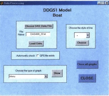
the display of many windows (one window for each type of data: accelerations, rotations rate etc. .. ), a Matlab Graphical User Interface was built to facilitate the task. The GUI window is

SENSORS 2.4 Data Processing Program

Figure 2-6: Matlab Graphical User Interface for data processing

For each test, at least three logfiles were available: one with DMU and Magnetometer data, another containing commands sent to the MEI card and a third one containing the MEI card data (data sent to the motors). For tests where the GPS signal could be received (outdoors conditions, Hanscom swimming pool), a GPS logfile was also available.

The functionalities of the GUI are the following:

" easy window management: all the data plots do not appear at once, the user actually

chooses which windows are displayed,

" possibility of plotting several sets of data on the same figures, each set of data being

displayed with a specific type of drawing line.

" automatic check if a GPS logfile exists, the Menu displaying the list of figures available

for plotting being updated in consequence. Available choices

are-2.4 Data Processing Program

SENSORS 2.4 Data Processing Program

SENSORS 2.5 Summary

without GPS: 1. Magnetometer raw/filtered data

2. DMU raw/filtered accelerations

3. DMU raw/filtered rotation rates

4. DMU filtered yaw rate

5. DMU Stabilized angles (roll/pitch)

6. DMU heading variation 7. Surge and Sway Velocities

8. DMU path

9. MEI data

10. MEI commands

with GPS:

same as without GPS plus:

11. GPS heading

12. DMU/GPS/Magnetometer headings

13. GPS trajectory

14. GPS+DMU trajectories 15. GPS velocity

* a summary graph containing the following plots: accelerations, rotation rates, stabilized angles, heading , surge and sway velocities and finally the ship model path.

2.5

Summary

This chapter was dedicated to the study of the three sensors which equip the boat: the mag-netometer, the DGPS and the 6-axis inertial unit. The understanding of their working is a key to being able to analyze the behavior of the boat during any testing. All the equations to con-vert the analog data which are logged by the ship model software were presented. Particularly, one has to be very careful on the position and orientation of each sensor frame with respect to the ship model frame.

Chapter 3

DESIGN OF A HEADING

CONTROLLER

3.1

Ship Steering Equations

3.1.1

Non-Linear Ship Steering Equations

Considering motions in the horizontal plane (i.e. 0 = 0 = p = q = w = 0, parameters defined on Figure (3-1)), also supposing the ship symmetric about the x-z plane and neglecting the influence of the vertical position of the center of gravity zG, the ship equations are:

X = m( - rv - xGr2) (3.1)

m( +ru+xG)

3.2)

N =Izz + MXG ( + ru) (3.3)

at

a

3.1.2

Linear Ship Steering Equations

In the previous equations, supposing the forward velocity of the ship is constant and equal to Uo and neglecting second order terms, the linear ship steering equations can be written

I EinI!Iin EI m ~ - -~ - - -

-DESIGN OF A HEADING CONTROLLER 3.1 Ship Steering Equations

X

p (roll angle)

... u (surge)

0 (pitch angle)

v (sway)

V

(yaw angle)

Earth Based Frame

r (yaw)

_1wvv

_x

YO

yZ w (heave)

0

_z

Y

8R>0

-r<O

-

--r

Figure 3-2: Rudder Position

as follows (cf [21]):

(3.4)

(3.5)

where v is the velocity along the y axis and r is the turning rate around the z axis assuming the sign conventions of a direct frame. The direct frame chosen is the frame illustrated on Figure

(3-1). The following linear decomposition of the hydrodynamic forces and moments is used,

keeping only the first order terms:

Y = Yb +Y+ +Yvv +Yrr +Y6R

N = N)b + Nr + Nvv + Nrr + NJR

(3.6)

(3.7)

where JR is the rudder angle, positive if the rudder is turned to port. The rudder angle

m(i) + Uor + xG0)

DESIGN OF A HEADING CONTROLLER 3.2 The Models of Nomoto

The yaw-sway equations can also be written in the following matrix form:

M + N = Rn

r r

the matrices being

M= m-Y m-Y#G

1

NY=

,

Y6

mxG - Nv Iz - Nr -N mxGUO - Nr N]

From those equation, the state-space model of yaw-sway movements is:

x = A x

+

where x is the state-space vector x = [v, r]T and A and bi are defined below:

A = -M-1 - N, b1 = M-1 - b

3.2

The Models of Nomoto

For more details about the models of Nomoto, references [10], [3] and [211 can be consulted.

3.2.1 Nomoto's Second Order Model

To obtain a direct relationship between the rudder angle JR and the turning rate r, the sway velocity can be eliminated in the two-variable Equations (3.4) and (3.5).

Thus, the Nomoto's second order transfer function between r and JR can be obtained:

_ KR(1 +Tas) r-(s) = 1 Ts(1 + TO) _(3.12) 6R (1

+

DESIGN OF A HEADING CONTROLLER 3.2 The Models of Nomoto

The parameters KR, T1, T2 and T3 of Nomoto's equation are defined by the following equations:

T1T2 = det(M) _det(N) (3.13) j11M22 + 22M21 - n12Tn21 ~~ n21M12 T1 + T2 = m det(N) (3.14) KR = n₂lb, - nub2 (3.15) det(N) KRT3 = - mub2 (3.16) det(N)

with mij and rij and bi are the elements of the matrices M, N and b defined in Equation

(3.9). Now, looking at how the angles have been defined (cf Figure (3-2)), a positive rudder

deflection implies a negative turning rate. However, the remote control system of the ship

model was designed such that the rudder angle is positive when the two rudders are turned to

starboard, so that when the rudder angle is positive the turning rate of the boat is also positive. Consequently, in order to design a controller that is compatible with those requirements, the following modified model will be used:

K = -KR, = -JR (3.17)

The time domain equation for the turning rate r is:

T1T21 + (Ti + T2)i- + r = K(6 + T36) (3.18)

The transfer function between r and J is:

r

(S)

+

6 (1+ Tis)(1 ₊ T2s)

The transfer function between 6 and the heading angle

(

S=

+

s s(1 + Tis)(1 + T2s)

Consequently, Nomoto's second order model is represented mainly by 4 coefficients:

9 three time constants: T1, T2 and T3. Usually, Ti is bigger than T2 and T3. Also, T2

DESIGN OF A HEADING CONTROLLER 3.3 Hydrodynamic Coefficients

e one turning ability coefficient K.

3.2.2 Nomoto's First Order Model

The simplification of the previous model was made by Nomoto and al. on the assumption that steering motions of ships are substantially first order phenomena. Consequently, the unique time constant T has to be chosen so that the first order simulating system coincides with the ultimate phase of the second order model. Nomoto and al. (cf. [10]) showed that the resulting simulation is satisfactory for a ship with relatively small T₁.

The goal of this first order model is to describe the steering qualities of ships with only two fundamental indices:

" an index of turning ability (K),

" an index of quick response in steering and the dynamic stability on course (T)

Nomoto's first order model is simply obtained by approximating the previous model using the effective time constant T = T1 + T2 - T3. The equations of this model are:

e Time domain equation:

Tr+r=K or T + b=K6 (3.21)

o Transfer function equation:

r K K

-(s) = or -(S) K (3.22)

j Ts+1 I s(Ts +1)

However, according to [3], the first order model should only be used at low frequencies. The models of Nomoto are very simple models and thus very useful to describe the heading as a function as the rudder angle. The next step in building the controller is to find the K and T coefficients using the hydrodynamic coefficients of the model DDG51 and experiments realized in [17].