Image description with generalized pseudo-Zernike moments.

HAL Id: inserm-00133663

https://www.hal.inserm.fr/inserm-00133663

Submitted on 6 Nov 2007

HAL is a multi-disciplinary open access archive for the deposit and dissemination of sci-entific research documents, whether they are pub-lished or not. The documents may come from teaching and research institutions in France or abroad, or from public or private research centers.

L’archive ouverte pluridisciplinaire HAL, est destinée au dépôt et à la diffusion de documents scientifiques de niveau recherche, publiés ou non, émanant des établissements d’enseignement et de recherche français ou étrangers, des laboratoires publics ou privés.

Image description with generalized pseudo-Zernike

moments.

Ting Xia, Hongqing Zhu, Huazhong Shu, Pascal Haigron, Limin Luo

To cite this version:

Ting Xia, Hongqing Zhu, Huazhong Shu, Pascal Haigron, Limin Luo. Image description with general-ized pseudo-Zernike moments.. Journal of the Optical Society of America. A Optics, Image Science, and Vision, Optical Society of America, 2007, 24 (1), pp.50-9. �inserm-00133663�

Image description with generalized pseudo-Zernike moments

Ting Xia

Laboratory of Image Science and Technology, Department of Computer Science and Engineering, Southeast University, 210096, Nanjing, China

Hongqing Zhu

Laboratory of Image Science and Technology, Department of Computer Science and Engineering, Southeast University, 210096, Nanjing, China

Huazhong Shu

Laboratory of Image Science and Technology, Department of Computer Science and Engineering, Southeast University, 210096, Nanjing, China

Centre de Recherche en Information Biomédicale Sino-français (CRIBs) Pascal Haigron

Laboratoire Traitement du Signal et de l’Image, Université de Rennes I – INSERM U642, 35042 Rennes, France

Centre de Recherche en Information Biomédicale Sino-français (CRIBs) Limin Luo

Laboratory of Image Science and Technology, Department of Computer Science and Engineering, Southeast University, 210096, Nanjing, China

Centre de Recherche en Information Biomédicale Sino-français (CRIBs)

Corresponding author: Huazhong Shu, Ph. D

- 1 -

HAL author manuscript inserm-00133663, version 1

HAL author manuscript

J Opt Soc Am A Opt Image Sci Vis 2007;24(1):50-9

This paper was published in Journal of the Optical Society of America. A, Optics, Image Science, and Vision and is made available as an electronic reprint with the permission of OSA. The paper can be found at the following URL on the OSA website:

Abstract

A new set of orthogonal moment functions for describing images is proposed. It is based on the generalized pseudo-Zernike polynomials that are orthogonal on the unit circle. The generalized pseudo-Zernike polynomials are scaled to ensure the numerical stability, and some properties are discussed. The performance of the proposed moments is analyzed in terms of image reconstruction capability and invariant character recognition accuracy. Experimental results demonstrate the superiority of generalized pseudo-Zernike moments compared with pseudo-Zernike and Chebyshev-Fourier moments in both noise-free and noisy conditions.

OCIS codes: 100.5010, 100.2960, 100.5760.

1. Introduction

In the past decades, various moment functions due to their abilities to represent the image features have been proposed for describing images.1-10 In 1962, Hu2 first derived a set of moment invariants, which are position, size and orientation independent. These moment invariants have been successfully used in the field of pattern recognition.3-5 However, geometric moments are not orthogonal and as a consequence, reconstructing the image from the moments is deemed to be a difficult task. Based on the theory of orthogonal polynomials, Teague6 has shown that the image can be easily reconstructed from a set of orthogonal moments, such as

Legendre moments and Zernike moments. Teh and Chin7 evaluated various types of image moments in terms of noise sensitivity, information redundancy and image description capability, they found that pseudo-Zernike moments (PZMs) have the best overall performance.

Recently, Ping et al.8 introduced Chebyshev-Fourier moments (CHFMs) for describing image. By analyzing the image-reconstruction error and image distortion invariance of the CHFMs, they concluded that CHFMs perform better than the orthogonal Fourier-Mellin moments (OFMMs), which was proposed by Sheng and Shen9 in 1994. Both CHFMs and OFMMs are orthogonal and invariant under image rotation.

In this paper, we propose a new kind of orthogonal moments, known as generalized pseudo-Zernike moments (GPZMs), for image description. The GPZMs are defined in terms of the generalized pseudo-Zernike polynomials (GPZPs) that are an expansion of the classical pseudo-Zernike polynomials. The two-dimensional (2D) GPZPs, ,are orthogonal on the unit circle with weights (1 – (zz*)1/2)α where

α

> –1 is a free parameter. The location of the zero points of real-valued radial GPZPs depends on the parameter

α

, so it is possible to choose appropriate values of

α

for different kinds of images. Experimental results demonstrate that the proposed moments perform better than the conventional PZMs and CHFMs in terms of image reconstruction capability and invariant pattern recognition accuracy in both noise-free and noisy conditions.

) , (_{z z}∗

V_pqα

The paper is organized as follows. In Section 2, we first give a brief outline of

PZMs. The definition of GPZPs, the corresponding weighted polynomials and the GPZMs is also presented in this section. Experimental results are provided to validate the proposed moments and the comparison analysis with previous works is given in Section 3. Section 4 concludes the paper.

2. Generalized pseudo-Zernike moments

In this section, we first give a brief outline of PZMs, they will also serve as a reference to compare the performance of GPZMs. We then present the GPZPs and establish some useful properties of them in the second subsection. The definition of GPZMs is given in the last subsection.

A. Pseudo-Zernike moments

The 2D pseudo-Zernike moment (PZMs), Zpq, of order p with repetition q is defined

using polar coordinates (r, θ) inside the unit circle as10,

θ

θ

θ

π

π rdrd r f r V p Z_pq 1 _pq( , ) ( , ) 2 0 1 0 *

∫∫

+ = , p = 0, 1, 2, …, ∞; 0 ≤ |q| ≤ p. (1) where * denotes the complex conjugate, and Vpq(r, θ) is the pseudo-Zernike

polynomial given by ) exp( ) ( ) , (r

θ

R r jq

θ

V_pq = _pq (2) Here R pq (r) is the real-valued radial polynomial defined as

₍

_{) (}

₎

p s q p s k pq r s q p s q p s s p r R − − =

∑

₋ − ₋ +₊ − _{+ −} = 0 ! | | ! | | 1 ! )! 1 2 ( ) 1 ( ) ( (3) The pseudo-Zernike polynomials satisfy the following orthogonality property

qk pl lk pq p rdrd r V r V

θ

θ

θ

π

δ

δ

π ) 1 ( ) , ( ) , ( 2 0 1 0 * + = ⋅

∫∫

(4)

where

δ

nm denotes the Kronecker symbol.

B. Generalized pseudo-Zernike polynomials

Wünsche11 recently presented the notion of generalized Zernike polynomials in the mathematical domain. Enlightened by the research work of Wünsche, we introduce generalized pseudo-Zernike polynomials with the notation in representation by a pair of complex conjugate variables (z = x + jy = r exp(jθ) and z* =

x – jy = r exp(–jθ)) and with real parameter

α

> –1 by the following definition ) , (z z∗ V_pqα ) ) ( 1 1 ; 1 ; 1 | | |, | ( |)! | ( ) 1 ( ) ( ) 1 ) ( 2 ( ) ( ) , ( 2 / 1 1 2 | | 2 / ) ( 2 / ) ( 2 / 1 ) 1 | | 2 , ( | | 2 / ) | (| 2 / ) | (| ∗ − − ∗ + ∗ + − − ∗ + ∗ − + − − − + − − + ⋅ = − ≡ zz q p q p F q p z z zz P z z z z V q p q p q p q q p q q q q pq

α

α

α α (5)

where denotes the Jacobi polynomials and 2F1(a, b; c; x) is the

hypergeometric function given by12

) ( ) , ( _u P_nαβ

∑

∞ = = 0 1 2 _{( ) !} ) ( ) ( ) ; ; , ( k k k k k k x c b a x c b a F (6)

Here (a)k is the Pochhammer symbol defined as

(a)_k =a(a+1)(a+2)...(a+k−1) with (a)0 = 1 (7) Using Eqs. (6) and (7), we obtain the following basic representation of GPZPs

2 / ) ( 2 / ) ( | | 0 1 2 1 | | * _{( )} )! 1 | | ( )! | | ( ! ) 1 ( ) 1 ( ) 1 ( )! 1 | | ( ) , ( p q p q s p q s s s p s q p pq z z s q p s q p s q p z z V + − ∗ − − − = − + + +

∑

− − + + − + − + + + =

α

α

α (8) In polar coordinate system (r, θ), Eq. (8) can be expressed as

) exp( ) ( )) exp( ), exp( ( ) , (

θ

α

θ

θ

α

θ

α _{r V r j r j R r jq} V_pq ≡ _pq − = _pq (9) where the real-valued radial polynomials Rα_pq(r) are given by

∑

− = − − + + + − − + + − + − + + + = | | 0 1 2 1 | | !( | | )!( | | 1 )! ) 1 ( ) 1 ( ) 1 ( )! 1 | | ( ) ( p q s s p s p s q p pq r s q p s q p s q p r R

α

α

α ₍₁₀₎

Comparing Eq. (3) with Eq. (10), it is obvious that

( ) ( ) (0,2| | 1)(2 1) (11) | | | | 0 _{= −} = + − r P r r R r R q q p q pq pq

Eq. (11) shows that the conventional pseudo-Zernike polynomials are a particular case of GPZPs with

α

= 0.

We now give some useful properties of radial polynomials Rα_pq(r).

a) Recurrence relations

The recurrence relations can be effectively used to compute the polynomial values. For radial polynomials given by Eq. (10), we derive the following three-term recurrence relations , for p – q ≥ 2 (12) ) ( ) ( ) ( ) (r M₁r M₂ R _1, r M₃R _2, r R_pqα = + α_{p− q} + α_{p− q} where ) )( 1 ( ) 2 )( 1 2 ( 1 q p q p p p M − + + + + + + =

α

α

α

(13) ) 1 2 ( ) 1 )( ( 1 ) 2 )( 1 ( 1 2

_α

_α

α

+ − − − + + + + + + + + − = p q p q p M q p p q p M (14) ) ( 2 ) 2 )( 1 )( ( ) 2 2 )( ( ) )( 1 ( 2 ) 1 2 )( 2 2 )( 1 )( ( 1 2 3

α

α

α

α

α

α

α

+ + − − − + + − + + + − + + + + + + + + − + − + + + = q p q p q p q p M q p p q p M q p q p p p q p q p M (15)

For the cases where p = q or p = q + 1, we have

q (16) qq r r Rα ( )= q q q q r q r q r R ( ) ( 3 2 ) 1 2( 1) , 1 = + + − + + + α α ₍₁₇₎

Note that the real-valued radial polynomials R_pqα (r) satisfy the symmetry

property about the index q, i.e., = , so that only the case where q ≥ 0 needs to be considered. ) (r Rα_pq ) (r ) ( , r R_pα_−q

The use of recurrence relations does not need to compute the factorial function involved in the definition of radial polynomials given by Eq. (10), thus decreasing the computational complexity and avoiding large variation in the dynamic range of polynomial values for higher order of p.

b) Orthogonality

The radial polynomials satisfy the following orthogonality over the unit circle Rα_{pq pl} q q lq pq q p p 2 ( + = p q α α 2)( | | ( + + − rdr r r R r Rα α α δ 1 | | 2 1 | | 2 1 0 1 | |) ) 1 ) 1 )( ( ) ( + + − + + −

∫

(18)

Eq. (18) leads to the following orthogonality of the GPZPs

[

]

pm qn q q mn pq q p p α π 2 ( 2 + + q p r r V r V δ δ α θ θ α α π α 1 | | 2 1 | | 2 * 1 0 2 0 2)( 1 | |) ) 1 | | ( ) 1 ( ) , ( ) , ( + + − + + + − −

∫ ∫

rdrdθ = (19)

The above equation shows that (1 – r)α is the weight function of the orthogonal relation on the unit circle, the integrals with such weight functions over polynomials within the unit circle converge in usual sense only for α > –1.

A usual way to avoid the numerical fluctuation in moment computation is by means of normalization by the norm. According to Eq. (18), we define the normalized radial polynomials as follows

1 | | 2 ) 1 | | 1 + + − + + q q p |)_{2| | 1} 2 ( ) ( ) ( ~ ₌ + q+ pq pq q p r R r Rα α | ( 2 )( 2 − + p π α α (20) Fig. 1 shows the plots of R~_pqα (r) with q = 10 and p varying from 10 to 14 for α being

0, 1 and 2, respectively. It can be observed that the set of radial polynomials R~_pqα (r)

is not suitable for defining moments because the range of values of the polynomials expands rapidly with a slight increase of the order. This may cause some numerical problems in the computation of moments, and therefore affects the extracted features from moments. To remedy this problem, we define the weighted generalized pseudo-Zernike radial polynomials by further introducing the square root of the weight as a scaling factor as

/2 1 | | 2 1 | | 2 ) 1 ( ) 1 | | ( 2 |) | 1 )( 2 2 ( ) ( ) ( α α α π α α r q p q p p r R r R q q pq pq _{− +} − − + + + + = + + (21) Fig. 2 shows the plots of weighted radial polynomials R_pqα (r) for some given orders

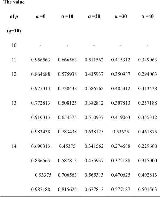
with different values of α. It can be seen that the values of the functions for various orders are nearly the same. This property is good for describing an image because there are no dominant orders in the set of functions V_pqα(r,θ) that will be defined below, therefore, each order of the proposed moments makes an independent contribution to the reconstruction of the image. Table 1 shows the zero point values of some weighted polynomials. It can be seen that the first zero point is shifted to small value of r as α increases. Moreover, the distribution of zero points for α between 10 and 30 is more uniform than α = 0. These properties could be useful for image description and pattern recognition tasks.

Let ) exp( ) ( ) , ( θ α θ α _{r R r jq} V_pq = _pq (22) we have

V_pq rθ V_nmα rθ rdrdθ δ_pnδ_qm π α ∗ ₌

∫∫

( , )[ ( , )] 2 0 1 0 (23)

C. Generalized pseudo-Zernike moments

The 2D GPZMs Z of order p with repetition q are defined as α_pq

θ θ θ π α α _{V r f r rdrd} Z_pq [ _pq( , )]* ( , ) 2 0 1 0

∫∫

= (24) The corresponding inverse transform is

( , ) ( , ) 0

θ

θ

_Zα_Vα _r r f p q pq pq

∑∑

∞ = = (25) If only the moments of order up to M are available, Eq. (25) is usually approximated by

∑

∑

∑

= > > ⎭⎬ ⎫ ⎩ ⎨ ⎧ + + = M p pq s q pq c q pq p c p R r Z q Z q R r Z r f 0 ) ( 0 ) ( 0 0 ) ( 0 ( ) 2 [ cos( ) sin( )] ( ) ) , ( ~

_θ

α α α

_θ

α

_θ

α ₍₂₆₎ where

θ

θ

θ

θ

θ

θ

π α α π α α rdrd q r f r R Z rdrd q r f r R Z pq s pq pq c pq ⋅ − = ⋅ =

∫∫

∫∫

) sin( ) , ( ) ( , ) cos( ) , ( ) ( 2 0 1 0 ) ( 2 0 1 0 ) ( q ≥0, (27)

For a digital image of size N × N, Eq. (24) is approximated by13, 14

( )exp( ) ( , ) ) 1 ( 2 1 0 1 0 2 R r jq f s t N Z N _{st st} s N t pq pq α

θ

α ₋ − =

∑∑

− = − = (28) where the image coordinate transformation to the interior of the unit circle is given by 2 1 , 1 2 , tan , ) ( ) ( _{1 2} 2 1 2 1 1 2 2 1 2 2 1 ⎟⎟ = ₋ =− ⎠ ⎞ ⎜⎜ ⎝ ⎛ + + = + + + = − _c N c c s c c t c c t c c s c r_st

θ

_st (29)

3. Experimental results

In this section, we evaluate the performance of the proposed moments. Firstly, we

address the problem of reconstruction capability of the proposed method, and compare it with that of CHFM. The recognition accuracy of GPZMs is then tested and compared with CHFM.

A. Image reconstruction

In this subsection, the image representation capability of GPZMs is first tested using a set of binary images. The GPZMs are computed with Eq. (28) and the image representation power is verified by reconstructing the image using the inverse transform (26). An objective measure is used to quantify the error between the original image f(x, y) and the reconstructed image fˆ(x,y), and it is defined as

∑∑

− (30) = − = − = 1 0 1 0 | )) , ( ˆ ( ) , ( | N x N y y x f T y x f

ε

where T(.) is the threshold operator

(31) ⎩ ⎨ ⎧ < ≥ = 5 . 0 0 5 . 0 1 ) ( u u u T

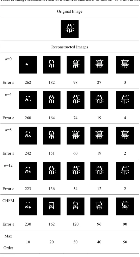
The uppercase English letter “E” of size 31 × 31 and a Chinese character of size 63 × 63 are first used as test images. Tables 2 and 3 show the reconstructed images as well as the relative errors for GPZMs with α = 0, 4, 8, 12, and CHFMs respectively. Other values of α have also been tested in this experiment, the detail reconstruction errors for GPZMs with α = 0, 10, 20, and CHFMs are shown in Figs. 3 and 4, respectively. As can be seen from the figures, the reconstruction error decreases for the same order of moment when the value of α increases. It can also be observed that the GPZMs (except for α = 0) perform better than the CHFMs, and the difference becomes more important when higher order of moments is used.

We then test the robustness of GPZMs in the presence of noise. To do this, we add respectively 5% and 10% of salt-and-pepper noise to the original image “E”, as shown in Figs. 5 and 6. The reconstruction errors for these two cases are shown in Figs. 7 and 8, respectively. The results show that the GPZMs with larger value of α produce less error when the maximum order of moments M is relative lower. Conversely, when the maximum order of moments used in the reconstruction is higher, the reconstruction error re-increases for larger value of α. This may be because the term (1 – r)α/2 appeared in the weighted radial polynomials is more sensitive to noise for large value of α. Another phenomenon that can be observed from these figures is that for a fixed value of α, the reconstruction error increases when the maximum order of moments M is higher. This is consistent with the conclusion made in the papers by Pawlak et al.15, 16 The reason is that higher order moments contribute to noise reconstruction rather than to the image.

B. Invariant pattern recognition

This subsection provides the experimental study on the recognition accuracy of GPZMs in both noise-free and noisy conditions. From the definition of the GPZMs, it is obvious that the magnitude of GPZMs remains invariant under image rotation, thus they are useful features for rotation-invariant pattern recognition. Since the scale and translation invariance of image can be achieved by normalization method, we do not consider them in this paper. Note that it is also possible to construct the rotation moment invariants that are derived from a product of appropriate powers of GPZMs17. However, the moment invariants constructed in such a way will have a large dynamic

range, this may cause problem in pattern classification. In our recognition task, we have decided to use the following feature vector taken into account the symmetry property of radial polynomials R_pqα(r)

V=[|Z₂₀α |,|Z₂₁α |,|Z₂₂α |,|Z₃₀α |,|Z₃₁α |,|Z₃₂α |,|Z₃₃α |] (32) where Z are the weighted GPZMs defined by Eq. (24). The Euclidean distance is α_pq

utilized as the classification measure

d (Vs, V t(k)) 2 (33) 1 ) ( ) (

∑

= − = T j k tj sj v v

where Vs is the T-dimensional feature vector of unknown sample, and V t(k) is the

training vector of class k. The minimum distance classifier is used to classify the images. We define the recognition accuracy η as 18

100% test in the used images of number total The images classified correctly of Number _× =

η

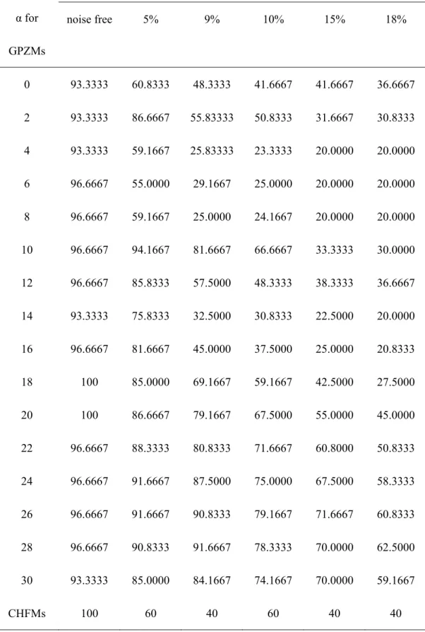
(34)

Two experiments are carried out. In the first experiment, a set of similar binary Chinese characters shown in Fig. 9 is used as the training set. Six testing sets are used, each with different densities of salt-and-pepper noises added to the rotational version of each character. Each testing set consists of 120 images, which are generated by rotating the training images every 15 degrees in the range [0, 360) and then by adding different densities of noises. Fig. 10 shows some of the testing images. The feature vector based on the weighted GPZMs with different values of parameter α is used to classify these images and the corresponding recognition accuracy is compared. The results of the classification are depicted in Table 4. One can see from this table that 100% recognition results are obtained, with α being 18 or 20, for noise-free images.

Note that the recognition accuracy decreases when the noise is high. Table 4 shows that the better recognition accuracy can be achieved for α between 20 to 30, and the corresponding results are much better than those with CHFMs.

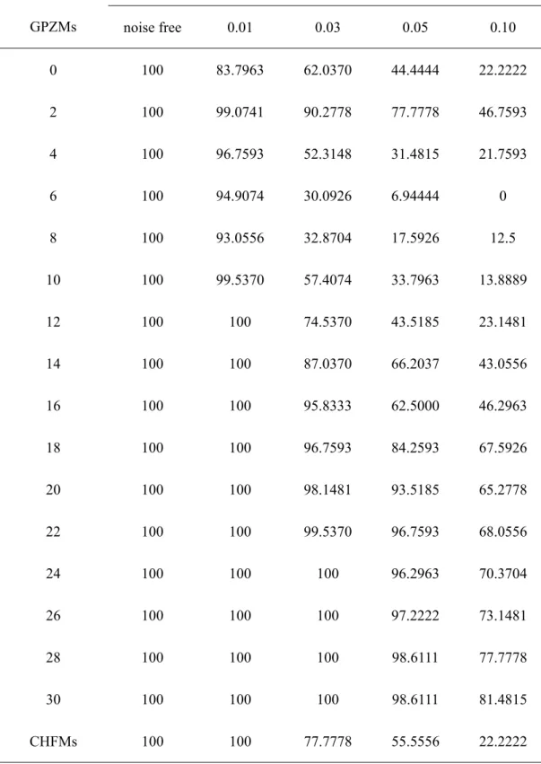
In the second experiment, we use a set of grayscale images composed of some Arab numbers and uppercase English characters {0, 1, 2, 5, I, O, Q, U, V} as training set (see Fig. 11). The reason for choosing such a character set is that the elements in subset {0, O, Q}, {2, 5}, {1, I} and {U, V} can be easily misclassified due to the similarity. Five testing sets are used, which are generated by adding different densities of Gaussian white noises to the rotational version of images in the training set. Each testing set is composed of 216 images. Fig. 12 shows some of the testing images, and the classification results are depicted in Table 5. Table 5 shows that the better results are obtained with α varying from 24 to 30.

4. Conclusion

We have presented a new type of orthogonal moments based on the generalized pseudo-Zernike polynomials for image description. We showed that the proposed moments are an extension of the conventional pseudo-Zernike moments, and are more suitable for image analysis. Experimental results demonstrated that the generalized Pseudo-Zernike moments perform better than the traditional pseudo-Zernike moments and Chebyshev-Fourier moments in terms of rotation invariant pattern recognition accuracy and image reconstruction error in both noise-free and noisy conditions. Therefore, GPZMs could be useful as new image descriptors.

Acknowledgements

This research is supported by the National Basic Research Program of China under grant 2003CB716102, the National Natural Science Foundation of China under grant 60272045 and Program for New Century Excellent Talents in University under grant NCET-04-0477.

References

1. R. J. Prokop and A. P. Reeves, “A survey of moment-based techniques for unoccluded object representation and recognition,” Comput. Vision Graph. Image Process. 54, 438-460 (1992).

2. M. K. Hu, “Visual pattern recognition by moment invariants,” IRE Trans. Inf. Theory IT-8, 179-187 (1962).

3. S. Dudani, K. Breeding, and R. McGhee, “Aircraft identification by moment invariants,” IEEE Trans. Comput. 26, 39-45 (1977).

4. S. O. Belkasim, M. Shridhar, and M. Ahmadi, “Pattern recognition with moment invariants: A comparative study and new results,” Pattern Recognit. 24, 1117-1138 (1991)

5. V. Markandey and R. J. P. Figueiredo, “Robot sensing techniques based on high dimensional moment invariants and tensor,” IEEE Trans. Robot Automat. 8, 186-195 (1992).

6. M. R. Teague, “Image analysis via the general theory of moments,” J. Opt. Soc. Am. 70, 920-930 (1980).

7. C. H. Teh and R.T. Chin, “On image analysis by the methods of moments,” IEEE Trans. Pattern Anal. Mach. Intell. 10, 496-513 (1988).

8. Z. L. Ping, R. G. Wu, and Y. L. Sheng, “Image description with Chebyshev-Fourier moments,” J. Opt. Soc. Am. A, 19, 1748-1754 (2002).

9. Y. L. Sheng and L. X. Shen, “Orthogonal Fourier-Mellin moments for invariant pattern recognition,” J. Opt. Soc. Am. A, 11, 1748-1757 (1994).

10. R. Mukundan and K. R. Ramakrishnan, Moment Functions in Image Analysis-Theory

and Application, (World Scientific, Singapore, 1998).

11. A. Wünsche, “Generalized Zernike or disc polynomials,” J. Comp. App. Math. 174, 135-163 (2005).

12. C. F. Dunkl and Y. Xu, Orthogonal polynomials of several variables, (Cambridge University Press, Cambridge, 2001).

13. C. W. Chong, P. Raveendran, and R. Mukundan, “The scale invariants of pseudo-Zernike moments,” Pattern Anal. Appl. 6, 176-184 (2003).

14. C. W. Chong, P. Raveendran, and R. Mukundan, “A comparative analysis of algorithms for fast computation of Zernike moments,” Pattern Recognit. 36, 731-742 (2003).

15. S. X. Liao, M. Pawlak, “On image analysis by Moments”, IEEE Trans. Pattern Anal. Mach. Intell. 18, 254-266 (1996).

16. S. X. Liao, M. Pawlak, “On the accuracy of Zernike Moments for Image Analysis”, IEEE Trans. Pattern Anal. Mach. Intell. 20, 1358-1364 (1998).

17. J. Flusser, “On the independence of rotation moment invariants”, Pattern Recognit. 33, 1405-1410 (2000).

18. P. T. Yap, P. Raveendran, and S.H. Ong, “Image analysis by Krawtchouk moments,” IEEE Trans. Image Process. 12, 1367-1377 (2003).

Tables

Table 1. Comparison of positions of the radial real-valued GPZP zeros with different α The value of p (q=10) α =0 α =10 α =20 α =30 α =40 10 - - - 11 0.956563 0.666563 0.511562 0.415312 0.349063 12 0.864688 0.975313 0.575938 0.738438 0.435937 0.586562 0.350937 0.485312 0.294063 0.413438 13 0.772813 0.910313 0.983438 0.508125 0.654375 0.783438 0.382812 0.510937 0.638125 0.307813 0.419063 0.53625 0.257188 0.355312 0.461875 14 0.690313 0.836563 0.93375 0.987188 0.45375 0.587813 0.706563 0.815625 0.341562 0.455937 0.565313 0.677813 0.274688 0.372188 0.470625 0.577187 0.229688 0.315000 0.402813 0.501563

Table 2. Image Reconstruction of the letter “E” of size 31×31 without noises Original Image Reconstructed Images α=0 Error ε 56 46 27 14 4 3 2 2 0 α=4 Error ε 47 31 16 4 3 2 2 0 0 α=8 Error ε 42 18 5 4 3 2 0 0 0 α=12 Error ε 29 13 4 4 2 0 0 0 0 CHFM Error ε 45 39 13 10 11 9 11 8 7 Max Order 4 6 8 10 12 14 16 18 20

Table 3. Image Reconstruction of a Chinese character of size 63×63 without noise Original Image Reconstructed Images α=0 Error ε 262 182 98 27 3 α=4 Error ε 260 164 74 19 4 α=8 Error ε 242 151 60 19 2 α=12 Error ε 223 136 54 12 2 CHFM Error ε 230 162 120 96 90 Max Order 10 20 30 40 50

Table 4. Classification results of the first experiment

Recognition accuracy ( %) under different salt and pepper noises Parameter α for GPZMs noise free 5% 9% 10% 15% 18% 0 93.3333 60.8333 48.3333 41.6667 41.6667 36.6667 2 93.3333 86.6667 55.83333 50.8333 31.6667 30.8333 4 93.3333 59.1667 25.83333 23.3333 20.0000 20.0000 6 96.6667 55.0000 29.1667 25.0000 20.0000 20.0000 8 96.6667 59.1667 25.0000 24.1667 20.0000 20.0000 10 96.6667 94.1667 81.6667 66.6667 33.3333 30.0000 12 96.6667 85.8333 57.5000 48.3333 38.3333 36.6667 14 93.3333 75.8333 32.5000 30.8333 22.5000 20.0000 16 96.6667 81.6667 45.0000 37.5000 25.0000 20.8333 18 100 85.0000 69.1667 59.1667 42.5000 27.5000 20 100 86.6667 79.1667 67.5000 55.0000 45.0000 22 96.6667 88.3333 80.8333 71.6667 60.8000 50.8333 24 96.6667 91.6667 87.5000 75.0000 67.5000 58.3333 26 96.6667 91.6667 90.8333 79.1667 71.6667 60.8333 28 96.6667 90.8333 91.6667 78.3333 70.0000 62.5000 30 93.3333 85.0000 84.1667 74.1667 70.0000 59.1667 CHFMs 100 60 40 60 40 40

Table 5. Classification results of the second experiment

Recognition accuracy ( %) under different σ2 _{Gaussian white noises}

Parameter α for GPZMs noise free 0.01 0.03 0.05 0.10 0 100 83.7963 62.0370 44.4444 22.2222 2 100 99.0741 90.2778 77.7778 46.7593 4 100 96.7593 52.3148 31.4815 21.7593 6 100 94.9074 30.0926 6.94444 0 8 100 93.0556 32.8704 17.5926 12.5 10 100 99.5370 57.4074 33.7963 13.8889 12 100 100 74.5370 43.5185 23.1481 14 100 100 87.0370 66.2037 43.0556 16 100 100 95.8333 62.5000 46.2963 18 100 100 96.7593 84.2593 67.5926 20 100 100 98.1481 93.5185 65.2778 22 100 100 99.5370 96.7593 68.0556 24 100 100 100 96.2963 70.3704 26 100 100 100 97.2222 73.1481 28 100 100 100 98.6111 77.7778 30 100 100 100 98.6111 81.4815 CHFMs 100 100 77.7778 55.5556 22.2222

Figure lists

1. Fig.1. The plots of normalized radial polynomials R~_pqα (r). Fig.1. a) α = 0;

Fig.1. b) α = 1; Fig.1. c) α = 2.

2. Fig. 2. The plots of weighted radial polynomials R_pqα(r)and their zero distributions with different values of α Fig.2. a) α = 0; Fig.2. b) α = 10; Fig.2. c) α = 20; Fig.2. d) α = 30; Fig.2. e) α = 40.

3. Fig. 3. Plot of reconstruction error for “E” without noise

4. Fig. 4. Plot of reconstruction error for the Chinese character without noise 5. Fig. 5. “E” added with 5% salt and pepper noises

6. Fig. 6. “E” added with 10% salt and pepper noises

7. Fig. 7. Reconstruction error for “E” with 5% salt and pepper noises 8. Fig. 8. Reconstruction error for “E” with 10% salt and pepper noises

9. Fig.9. Binary images as training set for rotation invariant character recognition in the first experiment

10. Fig.10. Part of the images of the testing set with 15% salt and pepper noises in the first experiment

11. Fig.11. Grayscale Images of the training set used in the second experiment

12. Fig.12. Part of the images of the testing set with σ2_{=0.10 Gaussian white noises in the}

second experiment

a) α =0

b) α=1

c) α=2

Fig.1. The plots of normalized radial polynomials R~_pqα (r).

Fig.2. a) α=0

Fig.2. b) α=10

Fig.2. c) α=20

Fig.2. d) α=30

Fig.2. e) α=40

Fig.2. The plots of weighted radial polynomials and their zero distributions with different values of α

Fig.3. Plot of reconstruction error for “E” without noise

Fig.4. Plot of reconstruction error for the Chinese character without noise

Fig.5. “E” added with 5% salt and pepper noises

Fig.6. “E” added with 10% salt and pepper noises

Fig.7. Reconstruction error for “E” with 5% salt and pepper noises

Fig.8. Reconstruction error for “E” with 10% salt and pepper noises

Fig.9. Binary images as training set for rotation invariant character recognition in the first experiment

Fig.10. Part of the images of the testing set with 15% salt and pepper noises in the first experiment

Fig.11. Grayscale Images of the training set used in the second experiment

Fig.12. Part of the images of the testing set with σ2_{=0.10 Gaussian white noises in the}

second experiment