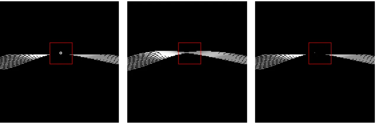
Strategy of computed tomography sinogram inpainting based on sinusoid-like curve decomposition and eigenvector-guided interpolation.
17
0
0
Texte intégral
Figure


Documents relatifs