A Half-Explicit Extrapolation Method for Differential-Algebraic Systems of Indix 3

A Half-Explicit Extrapolation Method for Differential-Algebraic

Systems of Index 3

ALEXANDER OSTERMANN

University de Genive, Section de mathimatiques, Case postale 240, CH-1211 Genive 24, Switzerland

[Received 1 May 1989]

The present paper is concerned with the numerical solution of differential-algebraic index 3 problems. We study an extrapolation method based on a variant of Euler's rule. This method only treats the algebraic variables implicitly, hence has computational advantages compared to fully implicit schemes. A numerical example in line with the theoretical results is included.

1. Introduction

IT is well known that extrapolation methods are an effective way to find the numerical solution of nonstiff and stiff differential equations with high accuracy, see Deuflhard (1985), Hairer, N0rsett, & Wanner (1987), Hairer & Lubich (1988), among others. In a series of papers several authors investigated the feasibility of extrapolation for the solution of differential-algebraic systems (Deuflhard, Hairer, & Zugck, 1987; Hairer & Lubich, 1987; Hairer, Lubich, & Roche, 1989; Lubich, 1989a). Yet, all methods considered in these articles were implicit or linearly implicit at least. Recently, Lubich (1989b) showed that Gragg's algorithm can be extended to index 2 problems in a quite direct way. The method retains the h2 expansion of the error and only treats the algebraic

components implicitly. A further extension to index 3 systems, however, does not seem to be possible without losing the h2 expansion. We shall therefore

generalize his ideas in another direction.

In the present article we propose an extrapolation method for index 3 problems that handles the differential components explicitly and only treats the algebraic variables implicitly, thus reducing the linear algebra considerably. In Section 2 we specify the class of differential-algebraic equations considered in this paper. We continue with a description of our basic method—a half-explicit Euler scheme—in Section 3. There we also prove the existence of an asymptotic expansion of the error, which gives the theoretical justification for extrapolation. In Section 4 we analyse the local error as well as the order of convergence for the resulting extrapolation method. A numerical example which is in line with the theoretical results is presented finally in Section 5.

It is worth mentioning that for the problems considered in this article the trapezoidal rule retains its h2 expansion of the error for the differential

components, but is only O(H) in the algebraic variables. The fully implicit midpoint rule, on the other hand, has no expansion at all.

2. Description of the problems to be studied

This paper treats the numerical solution of differential-algebraic systems of the form

y'=f(y,z), z' = k{y,z,u), 0 = g{y), (1) where /, k, and g have sufficiently many bounded derivatives. The system (1) is supposed to be of index 3 (in the sense of either Gear, Leimkuhler, & Gupta (1985) or of Hairer, Lubich, & Roche (1989)), i.e.

the matrix gy(y)fz{y, z)ku(y, z, u) has a bounded inverse

in a neighbourhood of the solution. (2a) (Here and in the following, partial derivatives are denoted by corresponding subscripts.)

Further it is assumed that k is linear in u, i.e.

k(y, z, u) = ko(y, z) + ku(y, z)u. (2b)

If one seeks a solution of (1) with an Euler-type method, this linearity assumption seems natural as it guarantees the existence of a solution for the implicit Euler discretization. (This subject is discussed in a remark following Theorem 6.1 in Hairer, Lubich, & Roche (1989).)

We suppose that the given initial values for the y and z components, y0 and ZQ

respectively, are consistent with (1), i.e.

«(*>) = o, gy(y0)f(yo,zo) = o. (2c)

Due to (2a, b), the initial value for the u component is uniquely determined by the relation

at the point (y0, ZQ, UQ). Anway, it will not enter the numerical method.

Examples for such index 3 problems are holonomic mechanical systems. As u normally plays the role of a Lagrange multiplier, its linear appearance is justified. For more details the interested reader is referred to Hairer, Lubich, & Roche (1989) and the literature cited there (e.g. Gear, Leimkuhler, & Gupta (1985) or Gear & Petzold (1984)).

3. h extrapolation for the half-expHdt Enler rule

For the numerical solution of (1) we consider the following half-explicit Euler rule

y*+i = y* + hf{yn, zn+l), (3a)

zn+1 = zn + hk(yn, zn, un+l), (3b)

0 = g(yn+i), (3c)

for n = 0 , 1,2,... .

The following theorem shows existence and uniqueness of the solution of (3) under appropriate assumptions.

THEOREM 1 Let (2) be satisfied in an h-independent neighbourhood of (r/, £) and assume that

Then the nonlinear system

y = ri + hf(ri,z), (4a)

2 = £ + hk(T,, £, u), (4b)

0 = g(y) (4c) possesses a unique solution for h «/i0, H>J//I u = 0(1).

Proof. Inserting (4a,b) into (4c) yields a nonlinear system for u

g(V + hf{t], t + hku(ri, £)«)) = 0, (5)

where t, = £ + hko{t], £). To study this equation, it is convenient to consider the

homotopy (as it is done in a similar way in Hairer, Lubich, & Roche (1989)) g(r, + hf{n, t + *«(»?> £)")) + (T - l)g(»J + A/(»J, f)) = 0. (6) For T = 0 a solution is given by v = 0. Note that for T = 1, (6) is equivalent to (5) with v = hu. We consider v as a function of x and differentiate (6) with respect to T. This yields

By assumption the second term is O(/i2), yielding the differential equation

&0» + hf(v, t + ku

(.n, 5)«))/z(»j, £ + *„(»?, £)«)*-(»?, £)o = o{h).

if = O(h)

and therefore

U(T) = \ v(t) dt = O(h) for Jo

Hence the differential equation possesses a solution at least for 0 «£ x « 1 and

hu = u(l) = O(h).

To prove uniqueness, we take a second solution & of (5) and denote the difference by Au = u — (L. Linearizing

0 = g(v + hf{n, t + hku(ri, Qu)) - g(ij + hf(ri, t + hku(V

immediately gives

and" hence Au = 0. Reinserting the unique solution u into (4b) and (4a) gives z and y explicitly. D

Remark. For the important special case—where / is linear in z—equation (5) can be solved by simplified Newton iterations with the A-independent matrix (gyfzku)(y0, ZQ) which is invertible by (2a).

Next, it will be shown that method (3) is well suited for h extrapolation. THEOREM 2 Under assumption (2) the method (3) is well defined for problem (1) for h small enough and its error possesses an h expansion of the form

Zn - z(xn) = h(bx(Xn) + ft) + - + h"(bN(Xn)

un - «(*„) = y° + h(cx(xn) + y\) + - + /."-'(

valid for 0 =£ nh =e const, with a^Xo) = 0, fi'n = 0 for n 5= 1, and •/„ = 0 for n 3= 2.

Proof. For the proof of Theorem 2 we shall use the ideas of Lubich (1989b) and Hairer, Lubich, & Roche (1989). The proof consists of two parts. First we will construct truncated expansions

xn)+ - + hN+1aN+l{xn),

K = u(xn) + y°n + h (C l( xn) + yl n) + • • • + h " ( cN( xn)

such that^o = >'o. ^) = ^o» and the defect of %+l, 2n+u un +, inserted into (3) is &+i = % + hf(Jn, fn+1) + O(hN+3),

2n+l = 2n+ hk(Jn, £„, an+l) + O(h"+2), (7)

The theorem then follows from a stability estimate given in (b).

(a) Truncated expansions: Inserting $n+l, 2n+u Qn+l, ?„, and 2n into (3) and

developing into Taylor series shows (writing fy(xn) instead of fy{y(xn), z(xn)),

etc.) + a[{xn) -fy(xn)ax(xn) -fz{xn)bx(xn) -fz{xH)z'{xn)] iym(xn) + \a\(xH) + a'2{xn) - fy(xn)a2(xn) - fz(xn)b2(xn) - \fz(xn)z\xn) -fz(xn)b[{xn) - ifM^))2 -fyz(xn)ai(xn)(z'(xn) + bM) - tfzz(xn)(z'(xn) + btix.))2] + O(h% 2n+i - £„ - hk(JH, £„, an+1) = hd^-ph - ku(x0)y'(\ + h2[\z"(xn) + b[(xn) - ky(xn)ai(xn) - kz(xn)b,(xn) - ku(xn)Cl(xn) - ku(xn)u'(xn)]

+ h26n0[-p2 - ku(x0)y\ - kz{x0)Ph - M*oK(*o)y? - ^«(Jto)(

+ h3[b2(xn) - ky(xn)a2(xn) - kz(xn)b2(xn) - ku(xn)c2(xn) - e2(xn)]

+ *3< U - 0 o " K(xo)y\ + e2] + O(h4),

= hgy(xn+i)a1(xn+l)

with the Kronecker symbol 6n0 (which is 1 for n = 0 and 0 otherwise). One

obtains (7) for N = 0 if

«!(*) =/,(*K0O +Ux)b1

(x) +f

(x)z'(x) - iy"(x),

b[(x) = k

(x)

(x) + *

(*)&ito + ku

(x)c,(x) + k

(x)u'(x) - iz"(x), (8)

0 = g

(x)a

(x),

k

(x

)tf=-pl (9)

After adding the component x' = 1, (8) is an index 3 system of the form (1). As in Hairer, Lubich, & Roche (1989) it is convenient to work with the projections

Q = Mxo)Mx0)/z(xo)fcu(xo)]-1sr(x0)A(x0) a n d P = I~Q Choosing

gy(xo)fz{xo)bx{xo) = hgy{x0)y\x0) - gy{x0)fz{x0)z'(x0),

gy(xo)fz(xo)ku(xo)cl(xo) = -gy(xo)/I(xo)61(xo) + hgy(xo)fz(xo)z"(xo)

gives consistent initial values for (8) and fixes Qbi(x0) as well as c^JCo). Now

multiplying equation (9) once with P and once with Q (and using Pku(x0) = 0)

determines the remaining coefficients of the expansion Pfi\ = 0, hence Pb^Xo) = 0 and

V? = \gy(Xo)fz(x0)ku(x0)]-lgy(x0)fz(x0)bl{x0).

The condition (7) for N = 1 yields a similar index 3 system for a2{x), b2{x), and

c2(x) with consistent initial values a2(x0) = 0 and gy(x0)fz(x0)b2(x0), c2(x0) suitably

chosen. To satisfy the equation

-p

+

(where er depends on known quantities only), we again apply P once and Q once,

Ppl = Peu ku(x0)Y\ = -QPl + Qe, = Qb2(x0) + Qex.

These conditions fix Pb2(x0) and yj. Repeating this procedure yields (7) for

arbitrary N.

(b) It remains to give the stability estimate. To this aim we will show inductively that the solution of (3) exists and that the differences Ayn+l =

y«+i-#.+i» etc. satisfy

Ayn+l = O(hN+l), Azn+l = O(hN+i), Aun+i = O(hN)

for nh =£ const.

By construction one has Ay0 = 0 and AZQ = 0. For the general step, one uses

inductively

yn = y(xn) + hax(xn) + O(h2), zn = z(xn) + O(h)

Thus, Theorem 1 guarantees a unique solution yn+i, zn+1, and un+1 of (3) and, as

un+l = 0(1) by Theorem 1, a Lipschitz condition for / and k immediately yields

the a priori estimates

Ayn+x = O(h), Azn+l = O(h).

Now linearizing the difference of (3) and (7) one obtains

Ayn+1 = Ayn + hft{fH, 2n+l)Azn+l + O(h \\Ayn\\ + h2 \\Azn+l\\) + O(hN+2), (10a)

hAzn+l = hAzn + h2ku(Jn, Sn)Aun+1 + O{h2 \\Ayn\\ + h2 \\Azn\\) +O(hN+3), (10b)

0 = & a+x ) ^ -+i + O(h \\AyH+1\\) + O(hN+2). (10c)

Inserting (10a) and (10b) into (10c) and extracting Aun+l from the resulting

equation gives

-h2(gyfzku)nAun+1 = {gy)nAyn + {gyfz)nhAzn

+ O(h \\Ayn\\ + h2 \\Azn\\) + O(hN+2) (11)

(with the notation (gyfI)n= gy($n)fz($n, £,)» etc.); Reinserting this into (10b) and

(10a) finally leads to the recursion

Ayn+l = (I-fzS)nAyn + (Jz)n(I - Sfz)nhAzn

+ O(h \\Ayn\\ + h2 \\Azn\\) + <Jzku)HO(hN+2) + O(hN+3), (12a)

hAzn+l = (/ - Sfz)nhAzn - Sn(J*S)HAyn

+ O(h \\Ayn\\ + h2 \\Azn\\) + (ku)nO(hN+2) + O(hN+\ (12b)

where S denotes the matrix kuigyf^y^gy. Now, direct application of Lemma 6.5 in Hairer, Lubich, & Roche (1989) gives the desired results

| | ^n + 1| | = O(hN+i), \\Azn+l\\ = O(hN+l),

and together with (10c) and (11) the estimate for the u component ||Aun+1|| = O{hN). D

4. Convergence of the extrapolation method

This section is devoted to extrapolation based on method (3). We want to investigate the local error as well as the order of convergence. To this aim we shall first define the extrapolation methods.

For a given sequence of positive integers nt < n2 < n3 < ••• and a basic stepsize

H>0, let hj = Hlnl denote the corresponding stepsizes and yh(x)=yn for

x =xo + nh. The tableau for h extrapolation is then given by

Each entry Tjk in this tableau can now be regarded as a numerical method for

solving equation (1). We shall denote this numerical solution at the gridpoints xo + mH by capitals Ym, Zm, and Um, componentwise. The aim of this section is

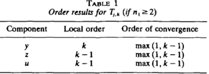
T A B L E 1

Component

y z u

Order results for

Local order k k-l k-l (ifn^l) Order of convergence max(l, max(l, max(l, k-l) k-l)

4.1 The Local Error

The assertion for the local error is proved by Theorem 2. If nx^2, each

extrapolation eliminates one power of h in the expansion of the theorem. Thus the local error satisfies

-[ z(x

+

H)

=

\ J '

(-1)*

/a

(x

+ H)\

b

(x

+ H) \

\c

(x

+ H)/

O(H

)

(cf. error formula for polynomial interpolation in Abramowitz & Stegun (1964: Formula 25.2.27)). Since ak(xo) = 0, the local error of the y component is

O(Hk+l), whereas it is O(Hk) for the other two components.

4.2 The Global Error

For k = 1 the result is an immediate consequence of Theorem 2. Therefore we have to consider k > 2 only. In this case the global error can be estimated by standard techniques like Lady Windermere's Fan (Hairer, N0rsett, & Wanner, 1987: p. 160). Figure 1 shows this fan for the y component.

To estimate the global errors Y°N-Y% and Z°N-Z% of the y and z

components, we analyse the propagation of the local errors, that means we

Xo+2H

estimate the differences Y'^1 — Y'N and Z'^x — Z'N in terms of the local errors

Y',~x - Y'I and Z',~l — Z1,. We suppose for a moment

\\g(Y'-1 + Hf(Y'-\ Z'-l))\\ « C0H2, \\g(Y'm + Hf{Y'm, Z'm))\\ « C0H2, (13)

which will be justified inductively below. Because of (13), Theorem 1 guarantees the existence of Y'~lu Y'm+U Z'~llt and Z'm+X. Using now the same techniques as

in the proof of Theorem 2, part (b), one can show that the differences AY*m+1 = Y'~li - Y'm+1 and AZ'm+l = Zl~\x - Z'm+1 satisfy again a recursion like

(12)—but with all derivatives now evaluated at the exact solution AVm+l = (/ -fzS)mAY'm + <Jz)m{l - Sfz)mHAZ'm

+ O(H\\AY'm\\+H2\\AZ'm\\), (14a)

HAZ'm+l = (/ - Sfz)mHAZ'm + Sm(JzS)mAY'm

+ O(H\\AY'm\\+H2\\AZ'm\\). (14b)

Application of Lemma 6.5 in Hairer, Lubich, & Roche (1989) with p = 0 thus yields, in the notation of Fig. 1,

and \\Z'^ - Z'N\\ *£ CHk. (15)

Summing up from / = 1 to N gives the order results for the y and z components as stated in Table 1.

To get the estimate for the u component we start with (10b). Using the notation of Section 3 for the current step at JC0 + mH we obtain

z)n(AZn+x ~ Azn) + O(Hk+2). (16)

To estimate the right-hand side, we multiply (10a) by (gy)n+\ which gives

0 = (gyUiAyn + h{gyfz)nAzn+, + h(gyfy)nAyn + O(Hk+2).

Here we used (gy)n+l = (gy)n + 0{h) and (gy)H+lAyn+l = O{Hk+2). Now

multiply-ing (10a) (for n replaced by n — 1) by (gy)n-u one similarly gets

(£y)n-lAyn =h{gyfz)nAzn + h{gyfy)nAyn + O{Hk+2).

A combination of the last two equations reads

h(gyfz)H(Azn+l - Azn) = -[(g,)f l +, + {gy)n-AAyn + O(Hk+2) = O(Hk+2)

which together with (16) implies the desired result

U'^-U'N = O(Hk). (17)

It remains to justify the assumption (13). By Theorem 2 it is satisfied for m = /. To treat the general case we use the fact that as long as Um - u(xo + mH) =

O(H), the constant Co does not affect the recursion (14). Thus, the constants in (15) and (17) can be chosen independently of Co> which justifies (13) recursively.

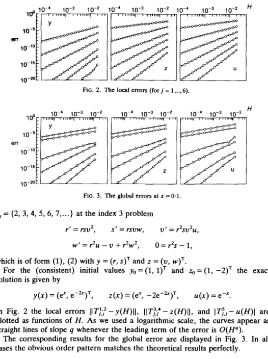
5. A numerical example

To show the relevance of our theoretical results to practical computations, we tested the extrapolation method (3) with the stepnumber sequence

,-2 H 10° 10- 5

en-ur

FIG. 2. The local errors (for/ = 1,._,6).

10"4 1(T3 10" 10~4 10"3 10" 10"s err 1 0 "1 0 1O"1S 1 0 "2 0 10"4 1 0 ^ 10" H

Fio. 3. The global errors at x = 0 1 . n, = {2, 3, 4, 5, 6, 7,...} at the index 3 problem

r = rsv , s = rsvw, v' = r2sv2u,

which is of form (1), (2) with y = (r, s)T and z = (t/, H»)T.

For the (consistent) initial values _yo = (l, 1)T and zo = (l,-2)T the exact

solution is given by

y(x) = (e*. z(x) = (e*, - u(x) = e"*.

In Fig. 2 the local errors \\T}?-y(H)\\, \\Tff- z(H)\\, and \Tjj- u(H)\ are

plotted as functions of H. As we used a logarithmic scale, the curves appear as straight lines of slope q whenever the leading term of the error is O(Hq).

The corresponding results for the global error are displayed in Fig. 3. In all cases the obvious order pattern matches the theoretical results perfectly.

Acknowledgements

I would like to thank E. Hairer and Ch. Lubich for their very helpful suggestions. They also gave the impetus for the present study.

This work has been supported by the 'Fonds national suisse de la recherche scientifique'.

REFERENCES

ABRAMOWITZ, M., & STEGUN, I. A. 1964 Handbook of Mathematical Functions. Dover Publ. Inc.

DEUFLHARD, P. 1985 Recent progress in extrapolation methods for ordinary differential equations. SIAM Review 27, 505-535.

DEUFLHARD, P., HAIRER, E., & ZUGCK, J. 1987 One-step and extrapolation methods for differential-algebraic systems. Numer. Math. 51, 501-516.

GEAR, C. W., & PETZOLD, L. R. 1984 ODE methods for the solution of differential/algebraic systems. SIAM J. Numer. Anal. 21, 716-728.

GEAR, C. W., LEIMKUHLER, B., & GUPTA, G. K. 1985 Automatic integration of Euler-Lagrange equations with constraints. /. Comp. Appl. Math. 12 & 13, 77-90.

HAIRER, E., & LUBICH, CH. 1987 On extrapolation methods for stiff and differential-algebraic equations. In: Numerical Treatment of Differential Equations (K. Strehmel, Ed.). Teubner-Texte zur Mathematik, Band 104.

HAIRER, E., & LUBICH, CH. 1988 Extrapolation at stiff differential equations. Numer.

Math. 52, 377-400.

HAIRER, E., LUBICH, C H . , & ROCHE, M. 1989 77K numerical solution of differential-algebraic systems by Runge-Kutta methods. Lecture Notes in Mathematics, vol. 1409,

Springer Verlag.

HAIRER, E., NORSETT, S. P., & WANNER, G. 1987 Solving Ordinary Differential

Equations I. Nonstiff Problems. Springer Verlag.

LUBICH, CH. 1989a Linearly implicit extrapolation methods for differential-algebraic

systems. Numer. Math. 55, 197-211.

LUBICH, CH. 1989b ^-extrapolation methods for differential-algebraic systems of index 2. To appear in IMPACT of Computing in Science and Engineering.