HAL Id: hal-02636464
https://hal.archives-ouvertes.fr/hal-02636464v3
Preprint submitted on 9 Jun 2020
HAL is a multi-disciplinary open access
archive for the deposit and dissemination of
sci-entific research documents, whether they are
pub-lished or not. The documents may come from
teaching and research institutions in France or
abroad, or from public or private research centers.
L’archive ouverte pluridisciplinaire HAL, est
destinée au dépôt et à la diffusion de documents
scientifiques de niveau recherche, publiés ou non,
émanant des établissements d’enseignement et de
recherche français ou étrangers, des laboratoires
publics ou privés.
A linearly polarized electromagnetic wave as a swarm of
photons half of which have spin –1 and half of which
have spin +1
Gerrit Coddens
To cite this version:
Gerrit Coddens. A linearly polarized electromagnetic wave as a swarm of photons half of which have
spin –1 and half of which have spin +1. 2020. �hal-02636464v3�
photons half of which have spin
−1
and half of which have
spin
+1
Gerrit Coddens
Laboratoire des Solides Irradiés,
Institut Polytechnique de Paris, UMR 7642,CNRS-CEA- Ecole Polytechnique, 28, Route de Saclay, F-91128-Palaiseau CEDEX, France
27th May 2020
Abstract. We illustrate our solution for the particle-wave duality and the paradox of the cat of Schrödinger on the example of the photons which occur in a linearly polarized electromagnetic wave. The +1 and −1 spin states correspond to the left and right circular polarizations, as pointed out by Raman and Bhagavantam [1]. This example provides also insight into the solutions of some other puzzles, e.g. how electromagnetic waves can propagate in vacuum, the supposed collapse of the wave function, the quantization of the electromagnetic wave, the reason for the Born rule and why we can solve quantum-mechanical wave equations by adopting boundary conditions that correspond to a coherent source even if the source is incoherent.
PACS. 03.65.-w, 03.65.Ca Quantum Mechanics
1 Schrödinger’s cat and the particle-wave duality
A stubborn problem in Quantum Mechanics1is the particle-wave duality, whereby it is proposed that a physical object like a photon or an electron can be both a particle and a wave, and that how it behaves depends on the experimental set-up. This is frankly incomprehensible, such that it has been often qualified as a quantum mystery. As this way of interpreting quantum mechanics is not satisfactory I thought we should find something more rational.2
In this document we will abandon the geometrical interpretation that electrons and photons would be both particles and waves and replace it by something that is more simple and free of mysteries. We will also provide a different geomet-rical interpretation for a wave function which is a superposition state of the type which occurs in the paradox of the cat of Schrödinger. Again, this will be much easier to make sense of.
The example of the double-slit experiment (e.g. for electrons) shows that the electrons reach the detector one by one as particles. The detector could e.g. be a photographic plate and one sees dot after dot appearing on the plate [2]. Therefore
1 In order to avoid all possible confusion I want to clarify the working assumptions underlying the present document. First of all we
are fully convinced of the fact that quantum mechanics and its algebraic rules to make the calculations are perfectly correct. To explain the fundamenta idea behind my endeavour it is perhaps good to consider an analogy. In algebraic geometry we define a correspondence between algebra and geometry, whereby everything in the geometry can be translated in a one-to-one fashion into algebra and vice versa. In quantum mechanics we perfectly know the algebra but the question how we should interpret it has not been settled. We do not know the geometry. In our analogy, we are looking for a geometry that would correspond to a more intuitive interpretation of quantum mechanics. We are thus not questioning quantum mechanics but only the way how it should be geometrically interpreted.
2 One could compare this particle-wave duality to what is claimed in the Christian religion: There is a Father, a Son and a Holy Ghost,
but there is only one God and this is a mystery. Dogmatic mystery is unacceptable in science. In fact, introducing such mysteries is a form of brainwashing. The person confronted with the contradictory “information” is startled and plunged into cognitive dissonance, because it is impossible to make sense of the contradiction which is imposed with authority as true. Taking advantage of this destabilization and the associated feeling of alienation, it becomes then easy to push him over into surrender mode. All this is typical of how authoritarian regimes install domination. In physics, the argument that a theory agrees with experiment is abusive and authoritarian when that theory is mathematically or logically ramshackle. Authority serves here to silence the questions the teacher himself cannot answer, because the problem of the meaning of quantum mechanics has never been settled. The teacher is now controlling the student’s mind and the indoc-trination can begin. Difficult challenging questions will no longer be asked, because the student has been made feel insecure and stupid. His only salvation to pass the examination will be to learn the stuff by heart and repeat it like a parrot. It is the better students who suffer from this the most.
2 G. Coddens: An electromagnetic wave as a swarm of photons
electrons are definitely particles. Gradually, after zillions of electrons have travelled through the double-slit the interference pattern appears. Contrary to what you have been told, this does not show that electrons are waves. It shows that the large number of electrons that have travelled through the set-up behaves like a wave. You should just sit down and reflect calmy about what I am telling you here to realize how you have been fooled with a leading argument. It is not the single electrons which are waves, it is the ensemble of electrons you have measured which looks like a wave. There is no need for theory to see that. All we need is serene unprejudiced observation. The conclusion is thus that electrons are particles and that it is the statistical ensemble of particles you have used in the experiment that behaves like a wave. This wave comes about without any interaction between the electrons, because one can assure that there is only one electron traveling through the set-up at the time. This is in marked contrast with a water wave, where the water molecules are also particles and not waves, but the macroscopic wave comes about by the interactions between these molecules. There must thus exist a phase relation between those electrons due to their initial conditions because you assume such a coherence for the wave.3There is then no longer a mystery. A wave function does thus never describe a single particle. It describes a statistical ensemble of particles. The wave function is a probability amplitude and probabilties are defined by considering the outcome of the experiment for a statistical ensemble of a large number of particles.4
It is therefore time to stop being cruel with cats. The wave function of Schrödinger’s cat does not describe a cat that is half alive and half dead. There are no such cats, because the wave function does not describe a single cat. It describes a statistical ensemble of cats. In this ensemble of cats, half of them are alive and half of them are dead. There is even a group theoretical justification for this solution of the paradox. There is a well-known argument due to Ehrenfest that a superposition state P
jcjψjdescribes an ensemble of particles whereby |cj|2are in the stateψj. We will now give a group-theoretical argument
to justify this for electrons. We propose to describe the spinning motion of the electron by spinors of SU(2) as described in [4]. In a group G, only one operation ◦ is defined, which one most of the time calls the product. In SU(2) the group is non-abelian and its 2 × 2 matrices represent three-dimensional rotations. The product of two group elements is defined, the sum is not. This is also true for rotations and especially for their representation matrices in SU(2). But in group theory, one nevertheless constructs all-commuting operators of a non-abelian group G. One considers then all operators of a same conjugacy class of elements h0= g ◦h◦g−1. Here h0and h are of the same conjugacy class, and g runs through G. Members of the same conjugacy class C are operations of the same geometrical type. E.g. they are rotations over the same angle but about different axes. The similarity transformation corresponds to a change of axis. An all-commuting operator is then defined as S =P
h∈Ch. This is
purely formal as the sum of group elements is not defined. And in textbooks one argues then ∀k ∈ G : k ◦ S = S ◦ k. It is a kind of annoying that this is purely formal, but it can be justified by proposing that k ◦ S = S ◦ k stands in reality for k ◦ C = C ◦ k, because the reasoning that occurs in both proofs is exactly the same. The latter identity is fully defined (k ◦C = {k ◦ g ∥ g ∈ C }) and exact.
This shows that a sum of group elements can be interpreted as representing a setS of group elements (in the example this is the conjugay class C ). By isomorphism, one can transpose this to the representation matrices D(g ). Then the sum P
g ∈SD(g ) stands for {D(g ) ∥ g ∈ S }. And we will have D(k)[Pg ∈SD(g ) ] = [Pg ∈SD(g ) ] D(k), when k ◦ S = S ◦ k. One can
now do the same with two electrons described by spinorsψ1andψ2of SU(2). The 2×1 spinors ψjare stenographic notations
for the 2×2 representation matrices D(gj) of group elements gj[5]. Hence we replace D(g1)|ψ1and D(g2)|ψ2, but we can then
no longer multiply to the right. And we have nowψ1+ ψ2as a representation of {g1, g2}. If there are 3 electrons that can be
described by g1and 2 electrons that can be described by g2, then {g1, g1, g1, g2, g2} (whereby the equal elements are tagged)
would describe this set of electrons and thus also 3ψ1+ 2ψ2. But in quantum mechanics there is now a twist, based on the
fact that ∀g ∈ G : [ψ(g )]†ψ(g) = 1. The spinors are normalized according to ψ†ψ = 1 because they represent SU(2) matrices. Hence counting a number of electrons cannot be done by adding quantitiesψ(g) but by counting quantities [ψ(g)]†ψ(g). Each count [ψ(g)]†ψ(g) = 1 counts one electron, the electron that tags g. We must thus count 3ψ†1ψ1+2ψ†2ψ2. And therefore
we must start from the set of quantities {p3ψ1,
p 2ψ2}, or
p 3ψ1+
p
2ψ2. Therefore, we come to the conclusion thatPjcjψj
represents a set of particles whereby |cj|2particles are in the stateψj, just as Eherenfest has told us. We have explained this
in more details in [5].
For photons the argument is different from the one for electrons. Here we use the idea that E2+ c2B2represents the total
energy. If the wave is monochromatic, all photons have the same energy and therefore E2+ c2B2is then a measure for the number of photons. In the Eq.1 below we haveψ†xψx= E2+c2B2, which represents the energy, and therefore also the number
of photons that contribute to this energy. Hence in both cases, the numbers of the particles in the states are proportional to
ψ†ψ. This can be considered as a derivation of the Born rule and the prescription of Ehrenfest. In the next Section we will
work out further the idea that photons are particles and that an electromagnetic wave must be a large collection of photons. The fact that we can succeed in working out this idea is in my opinion evidence for its validity.
3 IMPORTANT!!! Justifying that one can adopt boundary conditions that correspond to a coherent source, even when the source is
inco-herent, is a very important point, whose development we relegate to the Appendix, because it relies on a number of arguments that still have to be developed in the part of the main text that will follow.
2 Interpreting a linearly polarized electromagnetic wave as a swarm of photons
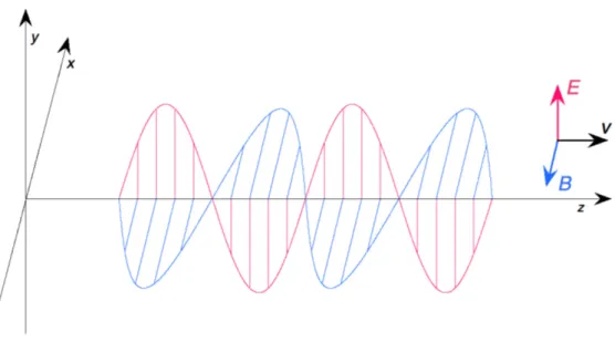
Fig. 1. Electromagnetic wave corresponding to Eq. 2.
We are used to discuss about polarizations of electromagnetic waves, but much less so about the spin of photons. Text-books tell us that photons have spin 1, which is puzzling, because this should lead to three substates with quantum numbers −1, 0, 1. But we only have linear polarizations −1 and +1. Where is the substate with quantum number zero? We will here explain the relationship between polarization and spin. It is important to have this connection, because in interactions we must be able to apply conservation laws. The basic quantity must therefore be the spin, not the polarization. We may note here that the discussion of the conservation law for spin and angular momentum is often tacitly omitted in text books of nuclear physics, which teach us e.g. the photoelectric effect or the Compton effect [6]. Only the conservation laws for energy and momentum are worked out. We are loosing some interesting information this way. Taking into account the conservation of spin and angular momentum shows that an electron must flip its spin when it absorbs a photon. This renders the abstract conservation law much more visual.
A linear polarization can be obtained as the superposition of two circular polarizations of opposite sign. If we accept that photons are particles with a spin then we must conclude that they must be circularly polarized such that a single photon can never have a linear polarization. It is only an ensemble of photons that can have a linear polarization. One should thus not try to derive Malus’ law in terms of photons that have a linear polarization. Just presenting photons with polarizations + or -as is done in the derivation of the Bell inequalities is also wrong (but this will not change the inequalities).
We will now try to understand how photons build an electromagnetic wave. We will consider first an electromagnetic wave that is linearly polarized along the x-axis and that propagates along the positive z-axis. The electric field and the magnetic field of a linearly polarized wave are in phase. Therefore we can have for the linear polarization along the x-axis in the Ox y plane: ψx= · Ex cBy ¸ = · E ıcB ¸ cos(ωt) (1)
We are expressing here the polarization with the aid of complex numbers. The y-direction corresponds then to the pre-factor
ı. By rotating this overπ/2 we obtain a linear polarization along the y-axis: ψy= · Ey cBx ¸ = · ıE −cB ¸ sin(ωt) (2)
4 G. Coddens: An electromagnetic wave as a swarm of photons
The electric and magnetic field are again in phase, but we are taking here sine waves in order to end up with dependences
e±ıωt later on.5Let us now construct the spin-up and spin-down states. This is just like a change of basis, but we will not
discuss the normalization of the basis vectors for the moment. We will just introduce some normalization here, and we will justify our choice later on. By summing we obtain:
ψL= 1 p 2(ψx+ ψy) = 1 p 2 · Ex+ Ey cBx+ cBy ¸ =p1 2 · E ıcB ¸ eıωt (3)
Now we add the factor that expresses the propagation along the positive z-axis. It must always have an argument with the combination kzz − ωt. But as we want to end up with a wave in eıωt we must thus take here the argument −(kzz − ωt).
ψL= 1 p 2(ψx+ ψy) = 1 p 2 · Ex+ Ey cBx+ cBy ¸ =p1 2 · E ıcB ¸ e−ı(kzz−ωt) (4)
By subtracting we obtain the other basis vector ( again not discussing its normalization):
ψR= 1 p 2(ψx− ψy) = 1 p 2 · Ex− Ey cBy− cBx ¸ =p1 2 · E ıcB ¸ e−ıωt (5)
We can finally add the terms that express the propagation along the positive z-axis:
ψR= 1 p 2(ψx− ψy) = 1 p 2 · E ıcB ¸ eı(kzz−ωt) (6)
Now if we want to go back to the original electromagnetic wave which is polarized along the x-axis, we have to take:
ψx=
1 p
2(ψL+ ψR) (7)
We assume now that each photon has an internal dynamics that generates an electromagnetic field which is (up the a nor-malization factor that gives it an energy ħω) the same as expressed in ψLorψR.6This way we can express the electromagnetic
wave as a swarm of photons where half of them have a left circular polarization and the other half a right circular polariza-tion. These left and right circular polarizations correspond to the spin states −1 and +1. We can now see the reason why we normalized withp1
2. In fact, when we have a superposition state cLψL+ cRψR, then the numbers of the photons in the states
ψLandψRare |cL|2and |cR|2. It is therefore that we must use the linear combinations:
ψx= 1 p 2(ψL+ ψR). (8) ψy= 1 p 2(ψL− ψR). (9)
This can be written as a transformation: · ψx ψy ¸ =p1 2 · 1 1 1 −1 ¸ · ψL ψR ¸ (10) The inverse transformation is then indeed:
· ψL ψR ¸ =p1 2 · 1 1 1 −1 ¸ · ψx ψy ¸ (11) This development must be seen as a simplifying Ansatz that solves a number of riddles of quantum mechanics in addition to those of the particle wave-duality and Schrödinger’s cat. It is the ensuing simplification that justifies it. First of all we can now clearly see that the electromagnetic wave is quantized. Secondly we can understand how an electromagnetic wave can propagate in vacuum. In principle there are no charges in vacuum. There is thus nothing the wave could jiggle to propagate itself. The wave propagates in the absence of any medium.7But by considering the wave as a swarm of photons, each of
5 In fact, as the polarization vector ofψ
yis just ı times the polarization vector ofψx, taking a cosine wave again would not lead to an
independent mode. Change from cosines to sines ensures independence.
6 Taking some liberties, we can express this by saying that the photon spins. This is analogous to the Ansatz that the electron spins
introduced in [4]. We are not able to to justify these assumptions by providing a dynamical model that would explain what produces the spinning motion. But in both cases we end up with a theory that is intelligible and reproduces the known theoretical results. The particles enter into a common descriptive framework. For the photon it is not possible to describe the spin dynamics in a co-moving frame as we did for the electron, because in the co-moving frame the time ought to be frozen.
which carries a small part of the field this conceptual problem disappears. This is perfectly analogous with the electrons in the double-slit experiment which traverse the set-up one by one without any interaction between them. They also do not need any medium to do their stuff like a sound or water wave. All they need is some clock of internal dynamics. Another problem that disappears is that of the collapse of the wave function, as in our approach all particles are always in well-defined places. The relationship between the photons and the wave is the same as in statistics when you make a histogram of a finite number of measured values and describe it by e.g. a continuous Gaussian distribution. The continuous wave function is a kind of coarse-grained mathematical ideal, suited to describe large ensembles of photons. Finally we would like to point out that also the electron wave function in the Dirac equation is a mixed state whereby the two components are obtained one from another by reflection (see [4], pp. 162-166).
If we want now a total of N photons in the wave at a certain spot r we must takepNψx(r). One may wonder why a photon
with spin 1 has only two substates −1 and +1. The reason for it will become clear in Section 3. It is because the linearly polarized electromagnetic wave has no zero-frequency component. As we can see on a drawing of such a wave in Fig. 1, it has nodes. The numbers −1, 0, and +1 do not have anything to do with some directions in space. They just correspond to frequencies (or actually to the prefactor m in eımφwithin the spherical harmonics Y`m(θ,φ), where we put φ = ωt in order to be able to use the mathematical tool to describe dynamics, just like we did for the electron in the Rodriguez formula). The waves are transverse. All the oscillations are inside a plane perpendicular to the direction of propagation. Therefore the group we must consider is the one of the rotations and reversals within the polarization plane. Rotations are obtained from an even number of reflections, while reversals are obtained from an odd number of reflections. These operations are abstract because they are not taking place in space-time but in the plane of electromagnetic polarization vectors.
If you consider a rotation as the product of an even number of reflections, then the state obtained by complex conjugation from it is the product of an odd number of reflections. In fact ı → −ı in eıφ→ e−ıφis a reflection with respect to the x-axis. The angular momenta are real, they can provide an optical torque and the effect of such torques has been measured[7]. They also play a rôle in selection rules for atomic transitions [1].
The 2 × 1 representations we developped above permit to calculate the numbers of the particles. Actually, a real wave would be described with a hull functionp
ρ(z), where ρ is the probability density, because the linearly polarized
electromag-netic wave will not have an infinite extent. It will rather be a wave train, with a coherence length. Herep
ρ(z) will only be
non-zero in some finite (moving) z-interval [z1, z2]. And you have then to normalize according to
Rz2 z1 Rx2 x1 Ry2 y1 ψ †ψdxd ydz = Nħω.
N would then be the total number of photons in the wave within the interval [ x1, x2] × [ y1, y2] × [ z1, z2], andρ = |ψ|2its
density. And the true wave will then be a kind of photon burst. We may note that the expressions forψL(r, t ) andψR(r, t ) do
not contain the variables x and y. The x and y coordinates can therefore be choosen at will. For the density this implies a homogeneous density throughout the planes z = K , where K is constant. Our wave function describes thus really a plane wave.
Let us remind that according to the group theory performing the sumψ1+ψ2of two spinors actually does not make sense
(See e.g. Ref [5]). An example is the sum of a spinorψ(s,2π) for a rotation around an axis s over an angle 2π and a spinor
ψ(s,4π) for a rotation around the same axis over an angle 4π. This sum is exactly zero and has no meaning whatsoever.
However when we have two photons, the wave functions contain the electric and magnetic fields of the photons and the fields of the photons would add up, if they were at exactly the same position at the same time. In general, this will not happen and the photons will be in different positions.
A number of properies, like Malus’ law, are rather easy to derive from a wave picture but much less so from a particle picture. Conceptually that made it difficult to solve the particle-wave duality for electromagnetic waves along the same line as for electrons. Interpreting the waves in terms of particles as we have done may be instrumental in figuring out a derivation based on the particle picture.
3 Fourier analysis
In the previous Section we have found the decomposition by a lot of guessing and intuition. When we go to more complicated situations that intuition may fail us. We therefore would like to replace it by a more algebraic approach. Let us try to find the decomposition by Fourier analysis. Let us first introduce the notation:
a = · Ex cBy ¸ , (12)
for the polarization vector ofψx. The Fourier coefficient for the e+ıφcomponent ofψxbecomes then:
1 2π Z 2π 0 ψx eıφdφ = a 2π Z 2π 0 cos(φ)eıφdφ = a 2π Z 2π 0 cos2(φ)dφ +ıa 2π Z2π 0 cosφsinφdφ =1 2a. (13)
6 G. Coddens: An electromagnetic wave as a swarm of photons 1 2π Z2π 0 ψx e−ıφdφ = a 2π Z2π 0 cos(φ)e−ıφdφ = a 2π Z2π 0 cos2(φ)dφ −ıa 2π Z 2π 0 cosφsinφdφ =1 2a . (14)
The Fourier coefficient for the e0ıφ= 1 component of ψxbecomes then:
1 2π Z 2π 0 ψx dφ = a 2π Z 2π 0 cos(φ)dφ = 0. (15)
The polarization vector ofψyis:
b = ıa = ı · Ex cBy ¸ = ı · E ıcB ¸ = · ıE −cB ¸ . (16)
We obtain for the Fourier component e+ıφofψy:
1 2π Z 2π 0 ψy eıφdφ = a 2π Z 2π 0 ı sin(φ)eıφdφ = a 2π Z 2π 0 ı cos(φ)sin(φ)dφ − a 2π Z 2π 0 sin2φdφ = −1 2a, (17)
for the Fourier xomponent e−ıφofψy:
1 2π Z 2π 0 ψy e−ıφdφ = a 2π Z 2π 0 ı sin(φ)e−ıφdφ = a 2π Z 2π 0 ı cos(φ)sin(φ)dφ + a 2π Z2π 0 sin2φdφ =1 2a, (18)
and for the Fourier component 1 = e0ıφofψy:
1 2π Z 2π 0 ψy dφ = a 2π Z 2π 0 ı sin(φ)dφ = 0. (19)
This justifies that photons with a quantum number 0 do not occur. As already stated, the electromagnetic wave has nodes, and therefore has no constant component. Finally, there is a renormalization to be done, because we must make the inten-sities comply with the rule that they are |cj|2rather than cj. We obtain then the same results as before. Independence of the
basis vectors corresponds here toR
ψ†
1ψ2dφ = 0 and normalization to R ψ †
1ψ1dφ = 1.
4 A remark on gravitons and gravitational waves
We think it could be useful to apply our solution of the particle-wave duality also to gravitons and gravitational waves even if we are not likely to be confronted with the issues of quantum mechanics in gravitation any soon. We consider thus the assumption that gravitons exist, which up to now has not been proved. The currently accepted notion is that gravitational waves are rippling the fabric of space-time. The point we want to make is that also gravitational waves do not need a medium. All they need is some periodic internal dynamics within the gravitons that can be used as a clock. These internal dynamics would mirror the dynamics you attribute to the wave. It could be done the same way by analyzing the polarizations of the waves like we did for electromagnetism.
Considering gravitational waves as deformations of space-time has one merrit: It is convenient. Since Euclid, geometry has become a part of mathematics, even if in the beginning it came from observation and was thus a kind of physics. The perfection of the theory was so great that it became considered as pre-existing any physics. It had become abstract and dematerialized. And in Newtonian physics it became a pre-existing playground which God had visited to lay down his laws of physics in it. We even thought at some point further back in time that the surface of the Earth was an infinite Euclidean plane, because our observations were too crude to notice the curvature. Only to find out later on that this infinite plane without curvature does not correspond to the physical reality and had been preconceived. The mathematics of this Euclidean plane were completely logical and contradiction-free, but they were not the mathematics that corresponded to the real situation. With the theory of relativity came the shock of realizing again that the Euclidean metric we had chosen for the vector space R4by which we presented space and time was perfectly logic and error-free but not the right one. But after that, the new
geometry, Minkowski’s space-time with it’s Riemannian pseudo-metric evolved again conceptually to the status of a perfectly logical pre-existing mathematical playground. But the lesson that we should have learned from special relativity is that space-time is created by electromagnetism. We are seeing straight lines because the atoms in the matter we use to visualize them are kept in place by electromagnetic interactions. It is the electromagnetic interactions which conjure up our perceptions of space and time. Space-time of special relativity is thus electromagnetic space-time. It is the space-time that corresponds to the invariance of the electromagnetic interactions. There is a deep connection between physics and the geometry we adopt to describe it and it is just not “geometry first”.
We must warn against the strongly suggestive character of geometrical theories that make them look as a piece of mathe-matics that pre-exists the physics. We can see that space-time cannot be the vector spaceR4we imagine it to be because the
Universe is expanding. Another idiosyncrasy introduced by this concept ofR4as a pre-existing mathematical playground for the laws of physics is the idea that the future would already exist. This takes the mathematical tool of the space-time vector spaceR4again really too serious. To define an infinite space-time vector spaceR4we would need to have clocks that are synchronized up to infinite distance. As Einstein synchronization must be carried out by sending light rays to and fro two observers, there is no way we can possibly achieve this. It is this synchronization procedure which is responsible for the su-perluminal phase velocity of the de Broglie waves. We must thus really keep in mind that space-time is a part of the physics, that it is created by the expansion of the Universe, starting from the big bang, and that it has to be a manifold rather than a vector space. General relativity states that space-time is curved. Our bodies, meter sticks or our tight ropes that we use to visualize a straight line would become curved if we were swirling around a very heavy object. It is then very practical to use the curves the objects are taking as geodesics in our calculations. The tight rope will still be as straight a thing as it gets. The curved geometry is really the best reference geometry we can use to describe our observations.
Describing things this way is really pragmatic. What it really acknowledges for is that two types of forces are shaping now our geometrical stage, rather than one. We can make the identification and claim that it is space-time which is curved. But this relies tacitly on the principle of equivalence, that all matter reacts the same way to gravity. If there were some type of matter that violates the equivalence principle, the universality of the geometry would break down. This shows that there is a tacit assumption underlying our philosophy. One can push this idea of universality to the limit where we consider that gravitational waves are deforming space-time, despite the fact that our local pragmatic choice of geometry ought to be flat because it is dominated by electromagnetism. That becomes then analogous to conceiving phonons in a crystal as deform-ing space-time, which is not truly convincdeform-ing an idea. Especially it conjures up the impression that space-time would be a medium like the aether, an elastic medium whose vibrations are the gravitational waves. That aether is now called the fabric of space-time. It could be wrong as many times before. We therefore think that it is better not to decide for the moment if this is true or otherwise. What we are arguing here is not a new theory, it is just a flashing warning light. One could wonder e.g. what our geometry would become when the four fundamental forces were acting at equal strength, or when gravitation overwhelms electromagnetism entirely like in a black hole. The way we cannot stop ourselves from falling into a black hole ressembles in this respect very much our notion of the passage of time. For the moment our choices do not have any prac-tical incidence on our physics. They are only changing the way we are telling the story. But we must be aware of the tacit assumptions that are underlying them. They could break down at some new stage of knowledge and then become an intel-lectual barrier against understanding the physics, just like Euclidean geometry was a conceptual barrier to be overcome in formulating relativity.
5
Appendix: Why we can use coherent-source boundary conditions for an incoherent source
What you do when you are solving a wave equation and impose the boundary conditions is assuming that the source is coherent.8We could e.g. consider plane waves impinging on a set-up, and then everywhere on the plane of the source, we would attribute the same phase to the particle by the boundary conditions. This is not self-evident because the source may be incoherent. This shows that in this kind of problem the phase itself is not important and that it is the phase difference built up starting from the source which counts. That is then the reason why we can act as though the source were coherent. It is this phase relation imposed at the source which applies then to all particles. In fact, we can put all initial phases equal to zero and keep in mind the error this induces. Then we can correct for this error again at the end. (If this were to be incorrect because e.g. an electron has undergone a spin flip during its trajectory, then the coherence of the wave solution would have been lost anyway). As what we finally measure is |ψ|2= ψ†ψ or |ψ|2= ψ∗ψ this will not change the experimental results. What counts in the end is the amplitude of the wave, not its phase.
This may sound absurd, because when you have two particles with dynamics described byψ1andψ2(e.g. within the
context of a Schrödinger equation), then correcting their phases byψ1→ ψ1eıα1andψ2→ ψ2eıα2, might destroy the
inter-ference inψ1+ ψ2: |ψ1+ ψ2|26= |ψ1eıα1+ ψ2eıα2|2. However, the idea that you should add up the two functionsψ1+ ψ2and
then square the result, is wrong and never applies. It belongs to the brainwash. Each particle must be counted in its own right, because the particles appear as dots on a detector screen one by one. Hence we must always determine the quantities of single particles according to |ψ1|2+ |ψ2|2, never according to |ψ1+ ψ2|2. When there is an interference pattern the weights
of the functionsψ1andψ2of two particles obey and comply already with the number of particles implied by the intensity
of the interference term |ψL+ ψR|2that you would write down according to the textbook rule, where R and L refer to the
left and the right slit, see Eq. 4 of Ref. [3]. E.g. if there were destructive interferenceψL(r) + ψR(r) = 0 there would be just
no particles described byψ1andψ2present in r, such that the weight coefficients c1(r) and c2(r) in c1ψ1+ c2ψ2would be
zero. To avoid confusion, it is perhaps instrumental to point out that we are considering hereψRandψLas spinor fields
con-structed from the histories of a huge set of particles j which have traveled through the set-up and whose individual dynamics
8 The situation addressed in this Appendix is different from the one of a coherent electromagnetic beam considered in the rest of the
paper. Here we consider the solution of quantum-mechanical wave equations, where one solves the equation by putting the phase at the source everywhere equal to zero.
8 G. Coddens: An electromagnetic wave as a swarm of photons
were described e.g. by spinorsψj(r, t ) along the paths r(t ), just like the electromagnetic wave is constructed from individual
photons.
If the particles are electrons and the wave functions are spinors of SU(2), the idea remains the same but the argument must be written differently, because the phases are rather changed by some rotationsψ1→ R1ψ1andψ2→ R2ψ2. The rest of
the argument remains mutatis mutandis the same because for the SU(2) matrices Rjwe have R†jRj=1. We can even consider
the case that the spins of the electrons emitted by the source are not aligned, but this is more elaborate. In fact, we must then reconstruct the SU(2) matrices D(g ) from their corresponding spinorsψ(g), develop the proof on the SU(2) matrices, and then switch back to the corresponding spinors in order to be able to derive the final result. The reason for this is that we can write a similarity transformation for the SU(2) matrices, but not for the spinors, because we cannot multiply a 2 × 1 spinor to the right with a 2 × 2 SU(2) matrix. The procedure to perform a similarity transformation on a spinor is visualized in the following equation and commuting diagram:
ψ(g) = · u v ¸ ↔ D(g ) = · u −v∗ v u∗ ¸ , ψ(g) ψ(h) y x D(g ) −−−−−−−−−−−−−−−−−→simililarity transformation D(g )→D(h)=R[D(g )]R−1 D(h) (20)
Within the context of the Dirac equation the analogous correspondence between the 4 × 1 spinors and the 2 × 2 repre-sentation matrices of SL(2,C) is given by Eqs. (4.9) and (5.58) in [4]. The relation between the 2×2 representation matrices of SL(2,C) and the 4×4 representation matrices in the Cartan representation of the Dirac formalism is also given in [4]. A change of axis s(g ) → s(h), embodied by a corresponding change of group elements g → h, is obtained by a similarity transformation D(g (0)) → D(h(0)) = R[D(g (0))]R−1, based on a rotation R. This will then evolve with time to D(h(t )) = R[D(g (t))]R−1(as proved in [4], pp. 310-313), whose spinorψ(h(t)) will comply now with the boundary conditions for a coherent source. The correction in the end to recover the correct incoherent-source value D(g (t )) = R−1[ D(h(t )) ] R is then just the reverse
similar-ity transformation. And then we will see that the spinorsψ(g(t)) and ψ(h(t)) will yield the same result [ψ(h(t))]†[ψ(h(t))] = [ψ(g(t))]†[ψ(g(t))] = 1. The main idea which makes this all work is that in a coherent process the spin axis does not change due to the interaction with the measuring device, else the process would be incoherent. A change of s would be accompanied with a corresponding change in the measuring device due to conservation laws. In the double-slit experiment this would e.g. permit to know through which slit the particle has gone. We may note that to our knowledge the issue that in general the source will be incoherent has never been addressed in examples of solving Schrödinger, Pauli or Dirac equations in textbook examples. The source has always been tacitly implied to be coherent by the choice of the boundary conditions. This has been then a kind of blind spot. The problem cannot be solved without a proper understanding of spinors and of the relationship between the particles and the waves. As said, what we are discussing here in this Appendix for wave equations is different from the situation we are studying in the rest of the document, which is that of a coherent electromagnetic beam.
References
1. C.V. Raman and S. Bhagavantam, Ind. J. Phys. 6, 353-366 (1931).
2. A. Tonomura, J. Endo, T. Matsuda and T. Kawaski, Am. J. Phys. 57, 647 (1986). 3. G. Coddens, ,https: //hal.archives−ouvertes.fr/cea−01459890v3
4. G. Coddens, in From Spinors to Quantum Mechanics, Imperial College Press, London (2015). 5. G. Coddens,https: //hal.archives−ouvertes.fr/cea−01572342v1.
6. P. Marmier and E. Sheldon in Physics of Nuclei and Particles (three volumes), Academic Press, New York, (1969). 7. Li He, Huan Li and Mo Li, Science Advances, 2(9), e1600485 (2016).