Development of a two-fluid, two-phase model for light water reactor subchannel analysis

FOR

LIGHT WATER REACTOR SUBCHANNEL ANALYSIS

by

JOHN EDWARD KELLY

B.S.N.E.,

University of Michigan, (1976} S.H., Massachusetts Institute of Technology, (1978)

SUBMITTED

IN

PARTIAL FULFILLMENT OF THE

REQUIREMENTS FOR THE

DEGREE OF

DOCTOR

OF PHILOSOPHY

at the

MASSACHUSETTS INSTITUTE OF TECHNOLOGY

AUGUST

1980

@

Massachusetts Institute of Technology

1980

Signatur.e of Author -

~~~nat~-~e

... _9_<1~8LIIIIC.,..te_d

______

_

Depart~t of Nuclear Engi~ng, August 8, 1980

Signature redacted

Certified by ,,,- ""' ---o~---0--#---T-h_e_s_i_s_S--up-e-.r-v_i_s_o_r

Signature redacted

Accepted by _ _ _ C_h_a_i_rm_a_n-,-b--D-e-~_..~-rt--~-e-rn-;-C-;nnn---g-t-t-.e-e_o_n_G_r_a_d_u_a_t_e_S_t_u_d~e-n_t_s

IRcHtV((J

rt-""'"'A "' "· •Mu.)

o~~T~~~1J&gi51;;u~

NOV

3

19SO

1.IBRARIES

DEVELOPMENT OF A TWO-FLUID, TWO-PHASE MODEL

FOR LIGHT WATER REACTOR SUBCHANNEL ANALYSIS

by

John Edward Kelly

Submitted to the Department of Nuclear Engineering on August 8, 1980 in partial fulfillment of the requirements for the Degree of Doctor of Philosophy in

Nuclear Engineering

ABSTRACT

The-problem of developing and assessing the two-fluid model computer code THERMIT for light water reactor (LWR) subchannel analysis

has been addressed. The developmental effort required a reformulation

of the coolant-to-fuel rod coupling so that THERMIT is now capable of

traditional coolant-centered subchannel analysis. A model that accounts

for mass, momentum and energy transport between mesh cells due to

turbulent mixing for two-phase conditions has also been introduced. This model is the first such attempt in a two-fluid context.

The liquid-vapor interfacial exchange terms in the two-fluid model have been modified for improved accuracy. A systematic evaluation

of the exchange models has been performed. The mass and momentum exchange rates between the vapor and the liquid for pre-CHF conditions were

evaluated by comparison to void fraction data in over 30 one-dimensional

steady-state experiments reported in the open literature. The

liquid-vapor energy exchange rate for post-CHF conditions was assessed using 15 steady-state, one-dimensional wall temperature measurements also found in the open literature. The two-phase mixing model has been evaluated using

G.E. and Ispra BWR and PWR rod-bundle measurements. Comparisons with these measurements have shown the appropriateness of this model. The assessment of the wall-to-coolant heat transfer model used steady-state, one-dimensional as well as transient, three-dimensional measurements. The comparisons resulted in a modification of the Biasi CHF correlation

to imptove 'its predictions.

THERMIT has been shown to accurately predict the thermal-hydraulic behavior of rod-bundles. Thus, it represents the first two-fluid computer code with this proven capability.

Thesis Supervisor: Mujid S. Kazimi

Title: Associate Professor of Nuclear Engineering

Thesis Reader: John E. Meyer..

ACKNOWLEDGEMENTS

The author would like to express his sincere gratitude to all those who assisted him in the preparation of this thesis. In particular, special recognition is given to the following individuals.

To Professor Mujid Kazimi who, as my thesis advisor has generously given his time and advice. _{His valuable comments and suggestions have}

greatly contributed to this thesis.

To Professor John Meyer who, as my thesis reader, has been very helpful during the course of this work.

To Professor Lothar Wolf, whose encouragement and advice have been greatly appreciated.

To Don Dube and Andrei Schor, who have shared with me many instructive discussions concerning THERMIT.

To Ping Kao, Samir Mohammed, Jim Loomis and Mahmoud Massoud who have assisted me in the computer related activities.

To Gail Jacobson and Riva Esformes who have typed this thesis.

To my wife, Sue, and all of my family whose constant encouragement and support have led to the successful completion of this work.

Finally, the financial support of Boston Edison Company, Consumers Power Company,.Northeast Utilities Service Company, Public Service

Electric and Gas.Company, and Yankee Atomic Electric Company under the sponsorhsip of the M.I.T. Energy Laboratory is greatly appreciated.

TABLE OF CONTENTS Section ABSTRACT ACKNOWLEDGEMENT S TABLE OF CONTENTS LIST OF FIGURES LIST OF TABLES NOMENCLATURE CHAPTER 1 - INTRODUCTION 1.1 Background 1.2 Research Objective 1.3 Development Approach

CHAPTER 2 - REVIEW OF PREVIOUS WORK

2.1 Introduction

2.2 Rod Bundle Analysis Techniques

2.2.1 Subchannel Analysis

2.2.2 Distributed Resistance Models

2.3 Two-Phase Flow Models

2.4 Description of THERMIT

2.4.1 Background

2.4.2 General Characteristics

2.4.3 Two-Fluid Model Conservation Equations 2.4.4 Finite Difference Equations

2.4.5 Constitutive Equations

CHAPTER 3 - DEVELOPMENT OF THERMIT SUBCHANNEL ANALYSIS

CAPABILITY 3.1 Introduction Page 2 3 4 7 12 14 17 17 19 21 23 23 29 29 32 33 35 35 35 38 40 49 52 52

Section

3.2 Geometrical Modeling Capability

3.3 Two-Phase Turbulent Mixing Model

3.3.1 Background

3.3.2 Model Formulation 3.3.2.1 Background

3.3.2.2 Analytical Formulation and

Discussion

3.3.2.3 Numerical Scheme

CHAPTER 4 - DEVELOPMENT AND ASSESSMENT OF THE

LIQUID-VAPOR INTERFACIAL EXCHANGE MODELS 4.1 Introduction

4.2 Assessment Strategy

4.3 Interfacial Mass Exchange

4.3.1 Background

4.3.2 Subcooled Vapor Generation Model

4.3.3 Droplet Vaporization Model

4.4 Interfacial Energy Exchange

4.5 Interfacial Momentum Exchange

CHAPTER 5 - ASSESSMENT OF THE TWO-PHASE MIXING MODEL

5.1 Introduction

5.2 G.E. 9 Rod Bundle Tests

5.2.1 Test Description

5.2.2 Single-Phase Comparisons 5.2.3 Uniformly-Heated Cases

5.2.4 Evaluation of Mixing Parameters

5.2.5 Non-Uniformly Heated Cases

Page 53 56 56 60 60 62 69 71 71 72 75 75 80 94 105 114 138 138 145 145 150 152 156 161

Section

5.3 Ispra BWR Tests

5.3.1 Test Description 3.3.2 Results

5.4 Ispra 16 Rod PWR Cases 5.4.1 Test Description 5.4.2 Results

5.5 Conclusions

CHAPTER 6 - THE HEAT TRANSFER MODEL

6.1 6.2 6.3 CHAPTER 7.1 Introduction Modifications Assessment 6.3.1 Steady-State Results 6.3.2 Transient Results

7 - CONCLUSIONS AND RECOMMENDATIONS

Conclusions

7. 2 Recommendations

REFERENCES

APPENDIX A DERIVATION APPENDIX B TWO-PHASE M

APPENDIX C HEAT TRANSFI

OF THERMIT GOVERNING EQUATIONS IXING MODEL ASSESSMENT RESULTS

ER CORRELATIONS 163 163 167 175 175 177 186 188 188 194 199 200 217 232 232 239 242 247 267 280

LIST OF FIGURES Figure 2.1 2.2 2.3 3.1 4.1 4.2 4.3 4.4 4.5 214-9-3

Fraction versus Enthalpy for Maurer 214-3-5

Fraction versus Enthalpy for Marchaterre

168

Fraction versus Enthalpy for Marchaterre 184

Temperature Comparisons for Bennett

5332

Temperature Comparisons for Bennett

5253

Temperature Comparisons for Bennett Case 4.6 Void Case 4.7 Void Case 4.8 Void Case 4.9 Wall Case 4.10 Wall Case 4.11 Wall Case 5442

4.12 Comparison of Wall Temperature Predictions Using Various r Models for Bennett Case 5332 4.13 Temperature Distributions for Subcooled Boiling

and Droplet Vaporization

Page 31 42 48 57 77 79 82 83

Coolant-Centered and Rod-Centered Layouts Typical Fluid Mesh Cell Showing Locations of Variables and Subscripting Conventions Typical Rod Arrangement in Transverse Plane

Illustration of Fuel Rod Modeling

Boiling Regimes in Two-Phase Flow in a Vertical Ttbe with Heat Addition

Illustration of Vapor Generation Rate, F, versus Equilibrium Quality, X

Illustration of Vapor Bubble Nucleation and Growth

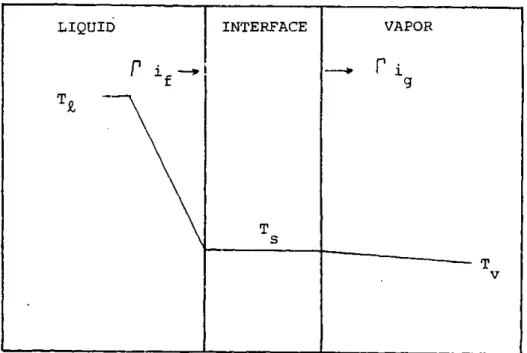
Typical Temperature Distributions in Subcooled Boiling

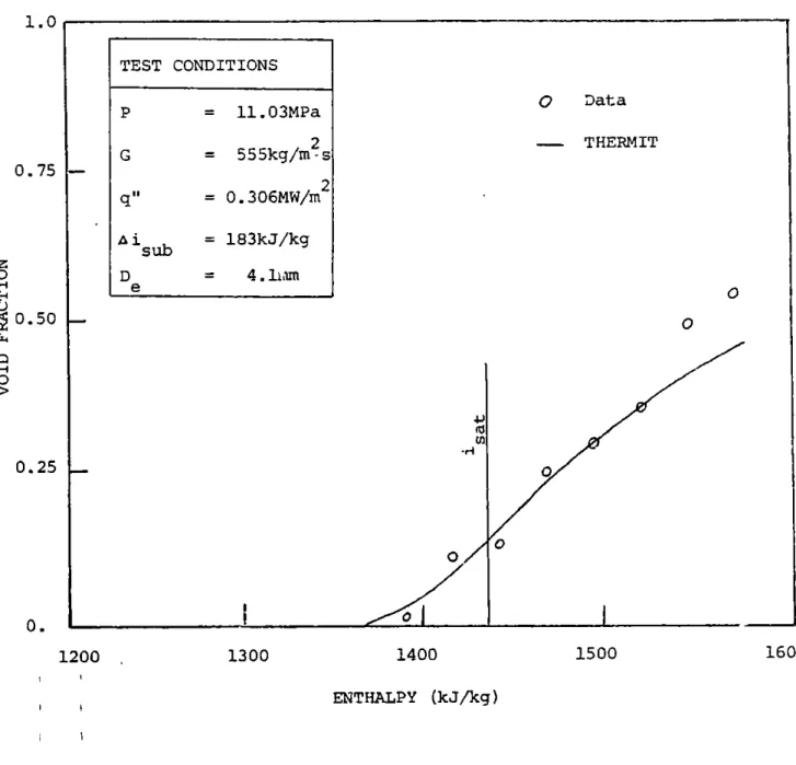
Void Fraction versus Enthalpy for Maurer

101 102 103 104 107 90 91 92 93

Figure Page

4.14 Predicted Liquid and Vapor Temperatures for l11

Maurer Case 214-3-5

4.15 Predicted Liquid and Vapor Temperatrues for 112

Bennett Case 5336

4.16 Typical Flow Patterns in Two-Phase Flow 115

4.17 Void Fraction versus Enthalpy for Maurer 129

Case 214-3-4

4.18 Void Fraction verius Enthalpy for Christensen 130

Case 12

4.19 Void Fraction versus Enthalpy for Christensen 131

Case 9

4.20 Void Fraction versus Enthalpy for Marchaterre 132

Case 185

4.21 Void Fraction versus Enthalpy for Christensen 134

Case 12

4.22 Comparison of Predicted Slip Ratios for 135

Christensen Case 12

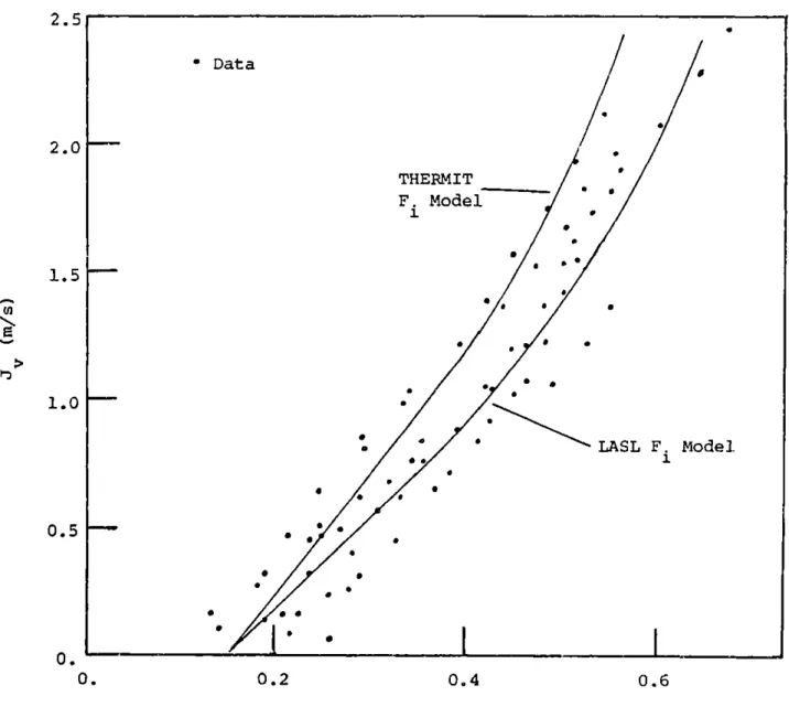
4.23 Vapor Superficial Velocity versus Void Fraction 137

for Christensen Data

5.1 Cross Sectional View of G.E. 9 Rod Bundle Used 146

in Mass Velocity and Enthalpy Measurements

5.2 Radial Peaking Factors for Non-Uniformly Heated 148

Cases

5.3 Comparison of Measured and Predicted Mass 151

Velocities for G.E. Isothermal Tests

5.4 Comparison of Measured and Predicted Exit Quality 153

in Corner Subchannel for G.E. Uniformly Heated

Cases

5.5 Comparison of Measured and Predicted Exit Quality 154

in Edge Subchannel for G.E. Uniformly Heated

Cases

5.6 Comparison of Measured and Predicted Exit Quality 155

in Center Subchannel for G.E. Uniformly Heated Cases

Figure

5.7 Comparison of Measured and Predicted Mass Velocities for G.E. Uniformly Heated Tests

5.8 Comparison of G.E. 2E Cases with 6M Varied

from I to 10

5.9 Comparison of THERMIT Predictions for Case 2E2 with Variations in KM

5.10 Comparison of Measured arid Predicted Quality for G.E. Non-Uniformly Heated Tests

5.11 Comparison of Measured and Predicted Mass Velocities for G.E. Non-Uniformly Heated Tests

5.12 Cross Sectional View of Ispra BWR Test Section

5.13 Comparison of Measured and Predicted Exit Quality

in Subchannel 2 - Ispra BWR Tests

5.14 Comparison of Measured and Subchannel I versus Bundle Ispra BWR Tests

5.15 Comparison of Measured and Subchannel 5 versus Bundle Ispra BWR Tests

5.16 Comparison of Measured and Subchannel 4 versus Bundle Ispra BWR Tests

5.17 Comparison of Measured and Velocities for Subchannels

BWR Tests

Predicted Quality for

Average Quality

-Predicted Quality for

Average Quality

-Predicted Quality for

Average Quality

-Predicted Mass 1 and 2 - Ispra

5.18 Comparison of Measured and Predicted Mass Velocities for Subchannel 4 and 5 - Ispra

BWR Tests

5.19 Cross Sectional View of Ispra PWR Test Section 5.20 Comparison of Measured and Predicted Exit

Quality for Subchannel 1 versus Bundle Average Quality - Ispra PWR Tests

5.21 Comparison of Measured and Predicted Exit Quality for Subchannel 2 versus Bundle Average Quality - Ispra PWR Tests

Page 157 159 160 162 164 165 169 170 171 172 173 173 176 179 180

Figure Page

5.22 Comparison of Measured and Predicted Exit 181

Quality for Subchannel 3 versus Bundle Average Quality - Ispra PWR Tests

5.23 Comparison of Measured and Predicted Exit 182

Quality for Subchannel 4 versus Bundle Average Quality - Ispra PWR Tests

5.24 Comparison of Measured and Predicted Exit 183

Quality for Subchannel 5 versus Bundle

Average Quality - Ispra PWR Tests

5.25 _{Comparison of Measured and Predicted Mass 184}

Velocities for Ispra PWR Tests

5.26 _{Comparison of Measured and Predicted Mass 185}

Velocities for Ispra PWR Tests

6.1 Typical Boiling Curve 189

6.2 BEEST Heat Transfer Logic 193

6.3 Modified Heat Transfer Logic 198

6.4 Typical Wall Temperature Distribution for 201

Bennett Case 5273

6.5 Comparison of Measured and Predicted Pre-CHF 203

Wall Temperatures for Bennett Case 5332

6.6 Comparison of Measured and Predicted Pre-CHF 204

Wall Temperatures for Bennett Case 5276

6.7 Comparison of Measured and Predicted Pre-CHF 205

Wall Temperatures for Bennett Case 5253

6.8 Comparison of Measured and Predicted Pre-CHF 206

Wall Temperatures for Bennett Case 5394

6.9 Comparison of Measured and Predicted Pre-CHF 207

Wall Temperatures for Bennett Case 5451

6.10 Illustration of Mass Velocity and Quality 213

Dependence of Biasi CHF Correlation

6.11 Cross Sectional View of G.E. 9 Rod Bundle Used 219

in Transient CHF Tests

6.12 Comparison of MCHFR Predictions versus Time for 221

Figure Page

6.13 Comparison of MCRFR Predictions versus 222

Time for Case 9-170

6.14 Comparison of MCEFR Predictions versus 223

Time for Case 9-175

6.15 Comparison of MCHFR Predictions versus 224

Time for Case 9-179

6.16 Comparison of Biasi Correlation Predictions 226

for Case 9-151 with Modified Grid Coefficients

6.17 Comparison of Biasi Correlation Predictions with 228

a Tighter Convergence Criterion (Case 9-179)

6.18 Comparison of Measured and Predicted Maximum 229

Wall Temperatures for Case 9-179

6.19 Comparison of Measured and Predicted Maximum 231

Wall Temperatures for Case 9-151

A.1 Illustration of Control Volume Containing 252

LIST OF TABLES

Tableage

2.1 Features of Some Thermal-Hydraulic Computer Codes 24

2.2 Thermal-Hydraulic Code Classification Criteria 25

2.3 Summary of Two-Phase Flow Models 27

2.4 Summary of Transport Processes 50

3.1 Implicit Heat Transfer Algorithm 55

4.1 Summary of Assessment P.rogram 74

4.2 Test Conditions for One-Dimensional Steady-State 89

Data

4.3 Test Conditions used to Develop Saha Correlation 97

for Post-CHF

4.4 Bennett Test Conditons for CHF in Tubes 100

4.5 Summary of Liquid-Vapor Intezfaciai Forces 121

4.6 Comparison of Viscous Force Coefficients 124

4.7 Comparison of Inertial Force Coefficients 126

5.1 Test Conditions for Rod-Bundle Experiments 143

6.1 Summary of Heat Transfer Correlations 192

6.2 CHF Comparisons for Bennett Test Cases 211

6.3 CHF Comparisons for Bennett Test Cases with 216

Corrected Biasi Correlation

6.4 Summary of Transient CHF Cases 218

7.1 Summary of Modifications and Improvements Made 233

in THERMIT

A.1 Summary of Terms Used in Conservation Equations 250

B.1 Test Conditions for- Rod-Bundle Experiments 268

B.2 Comparison of Measured and Predicted Exit Mass 269

Velocities for Isothermal Tests in 9 Rod G.E. Tests

B.3 Comparison of Measured and Predicted Exit Quality Distributions for Uniformly Heated 9-Rod G.E. Cases B.4 Comparison of Mass Velocity Heated Cases B.5 Comparison of Mass Velocity BWR Cases

Measured and Predicted Quality and Distributions for G.E. Non-Uniformly

Measured and Predicted Quality and Distributions for Ispra 16-Rod

c0.1 Heat Transfer Correlations

270

274

276

A Area Cd Drag Coefficient C Specific Heat D Diameter e Internal Energy F Gravitational Force

F _{Vapor-Liquid Interfacial Momentum Exchange Rate}

Ft Turbulent Momentum Exchange Rate

F Wall Frictional Force

g Gravitational Constant

G Mass Flux

H Heat Transfer Coefficient

i Enthalpy

J v Superficial Vapor Velocity

k Thermal Conductivity

K Mixing Model Parameter

M

L Length

P Pressure

Pr Prandtl Number

Qi

Interfacial Heat Transfer Rate

Qt Turbulent Heat Transfer Rate

QW Wall Heat Transfer Rate

i Power

q"I Heat Flux R b Bubble Radius

Nomenclature (continued)

Re Reynolds Number

S Slip Ratio (V /V

S ij Gap Spacing Between Coolant Channels

t Time

T Temperature

Td Bubble Departure Temperature

V Velocity

VR Relative Velocity (Vv - V)

W Volume

W' Turbulent Mixing Rate

WI" Turbulent Mass Flux t

W t Mass Exchange Due to Turbulence

X Quality

a Void Fraction

a Surface Tension

Parameter Defined in Eq. (3.33)

r Vapor Generation Rate

p Density

11 Viscosity

0 Mixing Model Parameter

E/ Turbulent Velocity

Generalized Mixing Rate Term

T Turbulent Shear Force

Subscripts i,j,k f g s v w Nodal Locations Saturated Liquid Saturated Vapor Liquid Saturation Vapor Wall Superscripts

x,y,z Spatial Directions

Anticipated Transient Without Scram Boiling Water Reactor

Critical Heat Flux

Critical Heat Flux Ratio Critical Power Ratio

Departure from Nucleate Boiling Loss of Coolant Accident

Light Water Reactor

Minimum Stable Film Boiling Pressurized Water Reactor Acronyms_ ATWS BWR CHF CHFR CPR DNB LOCA LWR MSFB PWR

1.0 INTRODUCTION

1.1 Background

Light water reactor safety research is ultimately aimed at ensuring that the public will not be adversely affected if any of a variety of

anticipated or postulated reactor accidents should occur. This

require-ment is met by specifying operational design limits that are based on

conservative assumptions for the behavior of the reactor. Reactor safety

research is primarily concerned with validating the appropriateness of these limits as well as assessing the margins- present in these limits.

In order to study the normal and abnormal transient behavior of nuclear reactors, many complex-phenomena and systems need to be analyzed. One of the major areas which must be investigated.:is the thermal-hydraulics of the reactor system. Included here are the reactor core heat removal

system, the secondary heat removal system (if present) as well as any

auxillary systems which are related to removal of heat from the reactor. Since most of the radioactive inventory is contained within the reactor

core, the preservation of the core integrity is essential. Moreove;,.the most likely radioactivity release mechanisms result from a thermally

induced failure of the fuel rod cladding. Thus, the thermal-hydraulic behavior of the core is generally the most important consideration of

reactor safety analysis.

In order to meet the objective of accurately predicting the thermal-hydraulic field in the reactor core a number of analytical tools have

been developed. These range from simple one equation models, used to predict a particular phenomenon, to large computer codes which attempt

to analyze the entire reactor system. Typically, the most widely used and generally the most useful tools are the thermal-hydraulic computer codes. Simply stated, these codes attempt to numerically solve the mass, momentum and energy conservation equations for a particular geometrical

configuration and for the conditions of interest. Since the conservation

equations must be supplemented by empirical correlations needed to describe specific phenomena, the thermal-hydraulic computer codes are engineering analysis tools which combine basic physics with empirical models.

In the past few years, the need for improved analysis of nuclear reactor safety has lead to the rapid development of advanced methods for

multidimensional thermal-hydraulic analysis. These methods have become

progressively more complex in order to account for the many physical phenomena which are anticipated during both steady-state and transient

conditions. In particular, the modeling of two-phase flow, which is

required for both BWR and PWR systems, is especially complex. In two-phase flows, both thermal and mechanical non-equilibrium between the two phases can exist. These non-equilibrium effects take the form of sub-cooled boiling, vapor superheating and relative motion of the two phases. In order to have realistic calculations, these physical phenomena must be accounted for in the numerical method.

The numerical methods must also be capable of analyzing the many

flow patterns which occur in postulated transients. For example, in a

loss of coolant accident (LOCA) or a severe anticipated transient without scram (ATWS), flow reversal or counter-current flow may occur in the

reactor core. Elaborate solution techniques have been developed specifi-cally to be able to describe fluid fields with no restriction on speed or direction.

cable for all transients, it is necessary that a code be able to analyze all anticipated flow conditions in problems for which the code is applied.

The only practical way to realize the needed flexibility is to combine

realistic physical models with unrestricitive numerical solution

techniques. Hence, the trend in current thermal-hydraulic safety research

is to pursue the development of such codes.

1.2 Research Objective

As discussed in the previous section, the thermal-hydraulic computer codes play a key role in LWR safety analysis. However, due to the limita-tions of present day computers, precise details of the thermal-hydraulic behavior can only be determined for a relatively small region of the

core. The response of the entire reactor can be determined if large

control volumes are used. However, within these volumes information

about the temperature and flow distribution is lost. If these distribu-tions are important for assessing the safety of the reactor, then detailed modeling is required. By using smaller control volumes, for example

sub-channels, sufficient temperature and flow information can be determined, but only for limited regions of the core. For instance, the largest

region which might be analyzed on a subchannel basis would be one BWR

8 x 8 assembly. Nevertheless, if the limiting region of the core can be identified, then this type of detailed analysis is sufficient to

evaluate the safety of the reactor.

A number of power and flow transients do require detailed subchannel

previous computer codes, which have used subchannel modeling, have either

lacked a realistic two-phase flow model (e.g. COBRA IV [1]) or lacked an

unrestricted solution technique (e.g. COBRA-IIIC [2]). Consequently, the

applicability of the previous codes is somewhat limited.

In view of the shortcomings of the previous codes, a new code which does not suffer from these deficiencies has been developed. Using the computer code THERMIT [31 as a framework, the present developmental effort has expanded the capabilities of THERMIT such that the new version of THERMIT can successfully analyze subchannel geometry [4].

THERMIT has been selected for this project due to its two-phase flow model and solution technique. The two-fluid, two-phase model which is used in THERMIT realistically allows for thermal and mechanical non-equilibrium between the phases. This feature permits description of the

complex phenomena encountered during transients. The solution technique

is a modification of the ICE method [5,6], and is capable of predicting

the flow conditions with minimum restrictions.

The primary application of this new version is transient analysis of

LWR rod bundles on a subchannel basis. Although depressurization

tran-sients (i.e. LOCA) have not been excluded as possible applications of this code, these transients are not the primary type of transient under

consid-eration. Rather, anticipated or near-operational power and flow transients

are the main focus of the present development considerations. By

concen-trating on non-depressurization transients, the code can be validated for

several practical conditions. Furthermore, the proper analysis of a LOCA

generally requires modeling the entire reactor system and THERMIT has been designed for core analysis only. Consequently, the applications for this new tool are limited to cases which can be analyzed by modeling only the

core and supplying appropriate core flow boundary conditions. Neverthe-less, these cases represent a large number of problems with practical interest.

With the ability to analyze subchannels, THERMIT is the first two-fluid model code with this capability. Due to the advanced treatment of the two-phase flow and reliable solution method, this code represents a significant addition to the area of rod-bundle thermal-hydraulic analysis. Other multi-fluid codes that may be used for subchannel applications are still under development at Argonne National Laboratory (COMMIX-2 (7-1) and Battle Pacific Northwest Laboratory (COBRA-TF [8]).

1.3 Development Approach

The development of this new version of THERMIT has been accomplished using the following strategy:

(1) Modify the code structure and numerical method as necessary,

(2) Verify, extend, and assess the constitutive models,

(3) Assess numerical properties of the code, and

(4) Implement improved models as necessary.

This strategy is actually iterative in nature. That is, as the need for improved models is found, code modifications and assessment are subsequent-ly required. Hence, the above steps overlap one another.

This development can be divided into two main steps. The first step

has involved modifying the original version of THERMIT so that subchannel geometry could be analyzed. This modification has affected both the geo-metrical modeling capability as well as the physical modeling. The

geo-metrical modeling changes were required so that the traditional

physical modeling wer necessary to account for turbulence effects in

single phase and two-phase flows for rod-bundle analysis. After reviewing

previous work in Chapter 2, the significant work related to this modifica-tion effort is discussed in Chapter 3.

After implementing the capability for subchannel analysis, the second

step has been the validation and assessment of the code. A strategy has

been adopted which allows for independent assessment of the various

con-stitutive models using open literature experimental measurements.

Measure-ments typical of expected subchannel conditions have been compared with the code's predictions in this effort. These comparisons are useful for both validating the predictive capability of the code as well as identi-fying areas which require improvement. The net result of this assessment effort is that the code can be used with confidence for subchannel appli-cations. The results of this assessment are discussed in Chapters 4, 5

and 6.

A listing of the actual computer code will not be given here due to

its length. Rather, the interested reader is referred to reference 9 which contains detailed information on the usage of this new version of THERMIT. Sample problems as well as input instructions are given in this

2.0 REVIEW OF PREVIOUS WORK

2.1 Introduction

Nuclear reactor thermal-hydraulic safety research encompasses both

experimental and analytical investigations. The experimental research

attempts to measure and identify the important variables in both

single-phase and two-single-phase flows. The analytical research attempts to develop

methods which numerically solve the equations describing the heat transfer and fluid dynamics in a reactor. Elabocate numerical methods have evolved which rely heavily on the use of digital computers. Conceivably, if all of the significant physical phenomena are considered in the computer code, then accurate predictions of the flow conditions can be obtained. These-methods can also analyze conditions which could not be directly measured. The only practical limitation of these methods is the problem

size which a computer can accomodate in terms of both storage and execution times.

Since this thesis has been concerned with the development of the

thermal-hydraulic computer code, THERMIT, it is instructive to review the

general characteristics of nuclear reactor thermal-hydraulic codes. The

key features of a few of these codes are presented in Table 2.1. As

discussed by Massoud [13j, it is possible to classify the codes according

to the criteria summarized in Table 2.2. The first major division is re-lated to the code's capability to handle one component or the entire by-draulic loop. Loop codes analyze a number of components simultaneously and,

Features of Some Thermal-Hydraulic Computer Codes

Computer Type of Method of Two-Phase Solution Technique

Code Analysis Analysis Flow Model

COBRA IIIC [2] Component Subchannel Homogeneous Equilibrium Marching Method

COBRA IV [1] Component Subchannel Homogeneous Equilibrium Marching Method or

I.C.E. Method

WOSUB [10] Component Subchannel Drift Flux Marching Method

COMMIX-2 [7] Component Distributed Two-Fluid I.C.E. Method

Resistance

THERMIT [3] Component Distributed Two-Fluid I.C.E. Method

Resistance

TRAC [12] Loop Distributed Two-Fluid or Drift Flux I.C.E. Method

Resistance

TABLE 2.2

Thermal-Hydraulic Code Classification Criteria

1. System Analysis Capability

A. Loop Codes

B. Component Codes

i. Subchannel Analysis

ii. Distributed Resistance Analysis

iii. Distributed Parameter Analysis

2. Two-Phase Flow Model

A. Homogeneous Equilibrium Model

B. Drift-Flux Model

consequently, analysis is not as detailed as found in the individual com-ponent codes. However, the component codes must have appropriate boundary

conditions supplied from external calculations. This prevents accurate

modeling of the coupling between the component and the rest of the system. Naturally, loop codes do not suffer from this problem.

Component codes, specifically those intended for rod-bundle analysis, can be further classified according to their analysis method. This

topic has been reviewed by Sha [14]. Three types of methods can be

identified; subchannel analysis, distributed resistance analysis and

dis-tributed parameter analysis. Each of these analytical techniques has

certain advantages and disadvantages relative to the other methods.

Sub-channel analysis techniques permit fairly detailed analysis of the flow,

but are limited by inherent assumptions concerning the flow. Distributed

resistance methods can analyze either large or small regions but require

the accurate determination of the flow resistances. The distributed

parameter analysis method gives the most detail of the flow structure, but is limited to small regions. All gf the core component codes use

one of these three analysis techniques.

The second major division is the type of two-phase flow model. The

important types of models which have been incorporated into

thermal-hydraulic codes include the homogeneous equilibrium model (HEM), the drift-flux model, and the two-fluid model. Essentially, the type of

two-phase model refers to the number of conservation equations which are

used to describe the two-phase flow, as summarized in Table 2.3. As the

number of conservation equations increases, the number of constitutive

models also increases. However, with more equations, accurate results are more likely to be predicted for severe conditions. The more general

Summary of Two-Phase Flow Models [151

Two-Phase Conservation Equations Constitutive Laws Imposed Restrictions On:

Flow Model

Mass Energy Momentum F

Q

r

Q

Fi Phasic Phasic Phatic

W W Temperatures Velocities Distributions

Homogeneous 1 1 1 1 1 0 0 0 Equal Equal Uniform

Drift Flux 2 1 1 1 1 1 0 0 T -T Slip None

Relahion Relation

4 Equation 1 2 1 1 2 0 1 0 None Slip Uniform

Relation

Models 1 1 2 2 1 0 0 1 T -T₂ None Uniform

Relation

Drift Flux 2 2 1 1 211 1 0 None Slip None

Relation

5 Equation 2 1 2 2 1 1 0 1 T -TR None None

Relation

Models 1 2 2 2 2 0 111 None None Uniform

Two-Phase Conservation Equations Constitutive Laws Imposed Restrictions On:

Flow Model

Mass Energy Momentum F 1 P Q F Phasic Phasic Phasic

Temperatures Velocities Distributions

Two-Fluid 2 2 2 2 2 1 1 1 None None None

Three-Fluid 3 3 3 3 3 2 2 2 None None None

(Liquid,

Vapor and

Liquid Drops)

equations also allow better physical modeling which is essential for the description of two-phase flow.

Since the present work is concerned with the application of the two-fluid model code THERMIT to detailed rod-bundle analysis, it is useful to discuss in detail both the type of analysis techniques and the two-phase

flow models. The analysis techniques are discussed in Section 2.2 while

the two-phase flow models are discussed in Section 2.3. Following this

discussion, the specifics of the THERMIT computer code will be given in

Section 2.4.

2.2 Rod-Bundle Analysis Techniques

As discussed in the previous section, three types of techniques are

available for rod-bundle analysis. These include subchannel analysis,

distributed resistance analysis and distributed parameter analysis. The

distributed parameter methods are limited to very small regions and will not be discussed here. The other two methods, however, are very useful for analyzing the entire rod-bundle and are discussed in detail.

2.2.2 Subchannel Analysis

Of all the methods developed for analyzing the thermal-hydraulic

behavior in complex rod-bundle geometry, the subchannel method has been found to be particularly well-suited. Weisman and Bowring [16] and

Rouhani (17] have reviewed this type of analysis and present the following

view of traditional subchannel analysis.

In this method, the rod-bundle cross section is subdivided into a number of parallel interacting flow subchannels. Conventionally these subchannels are defined by lines joining the fuel rod center (see Figure

2.la). This choice is somewhat arbitrary and other choices are possible,

such as the lines of zero shear stress (see figure 2.lb) [12]. This latter type of subchannel is referred to as a rod centered subchannel while the former type is called a coolant centered subchannel.

Once the radial plane has been defined, each subchannel is divided axially into a number of intervals (nodes) which are typically between

8 and 30 cm long. For each node, which can be thought of as a control volume, a set of mass, energy, axial momentum and transverse momentum conservation equations are written and solved with an iterative technique.

The main assumptions of this method are:

(1) The detailed velocity and temperature destributions within

a subchannel are ignored;

(2) The transverse nomentum equation is simplified due to the

assumption of predominantly axial flow.

The first assumption reflects the fact that only spatially averaged

parameters are contained in the conservation equations. Consequently,

the distributions within the control volume can not be calculated. The second assumption means that, due to the predominance of the axial flow, the transverse momentum exchange can be crudely represented without

introducing significant errors. Hence, the transverse momentum equation

is usuallr much simpler than the axial momentum equation.

A number of- computer codes have been developed which use the

sub-channel analysis method. Among these are included COBRA IIIC [2], COBRA-IV [1] and WOSUB (10]. These codes treat most of the

important phenomena in the same way and in each code a marching type

solution method is utilized. (COBRA-IV also contains a modified I.C.E. method [19] for transient analysis.) The marching method begins the

- I

-Figure 2.1b: Rod-Centered Subchannel Layout

.IMF-- nowalm--- Immmwmr

calculation of the flow parameters at the core inlet and moves upward,

in a stepwise manner, simultaneously solving the conservation equations for all subchannels, at each axial level. Typically, more than one sweep through the core will be required to obtain a converged solution.

Therefore, the marching method is basically an iterative technique.

For steady-state, single-phase conditions, the subchannel codes can generally predict the correct flow distributions in rod-bundles [16]. However, for two-phase conditions or severe transients, the use of the subchannel codes may not be strictly valid. For example, comparisons of COBRA-IIIC with steady-state two-phase flow measurements have indicated that the correct flow and enthalpy distributions could not be calculated

[10]. Also, if a strong perturbation causes large lateral flow, then the basic assumption in these codes is violated. Furthermore, if reverse flow should occur, then the marchiAg type solution method will fail

un-less appropriately modified. Consequently, although useful for many

rod-bundle problems, the subchannel codes are limited in their applica-tions.

2.2.2 Distributed Resistance Models

In order to eliminate the assumptions and restrictions of the

sub-channel methods, distributed resistance models have been developed. These

models also referred to as porous body models, use orthogonal coordinates and geometrically similar control volumes. The name for this method is

due to the fact that frictional resistances are distributed throughout

each of the control volumes. Quasi-continuum governing equations are

written for the conservation of mass, energy or momentum and no

no restrictions are placed on the flow conditions. However, as in the case of subchannel analysis, the details of the flow structure within a control volume cannot be determined.

By employing Cartesian coordinates, the geometrical noding of the

rod-bundle can be the same as for subchannel analysis (i.e., for square

bundles). Hence, the information obtained by the distributed resistance

method is at least as detailed as that found in subchannel methods. Of

course, the governing equations in the distributed resistance methods are more general than those in subchannel analysis methods.

However, the key to successful use of this method is the correct formulation of expressions for the transport processes in the control

volume (i.e., heat transfer, friction, etc.). These processes can be

described for most conditions, but completely general formulations are

noc possible. However, these processes can usually be defined for many

cases of practical interest.

A number of computer codes use the distributed resistance method.

Among these are COMMIX-1 [11], TRAC [121, and THERMIT [3]. Each of

these codes use some form of the I.C.E. solution technique [6]. This technique coupled to the full three-dimensional representation of the distributed resistance method allows for the calculation of flow reversal, recirculating flow and even counter-current flow in two-phase conditions. With the ability to analyze these conditions, the above codes represent

powerful tools for steady-state and transient thermal-hydraulic analysis

of rod-bundles.

2.3 Two-Phase Flow Models

important feature to be defined is the two-phase flow model. A wide variety of possibilities exist for describing the two-phase flow.

These range from describing the two-phase flow as a pseudo single-phase flow to a multi-component flow (e.g., liquid, vapor and droplets). The various possibilities are summarized in Table 2.3. Generally, as the

two-phase flow model becomes more complex (i.e., more equations), more constitutive equations are required to represent the various interactions between the phases.

The homogeneous equilibrium model (HEM) is the simplest of these models. It assumes that the vapor and liquid are in thermal equilibrium and that there is no relative velocity between the two phases. These assumptions are clearly limiting, but may be adequate for certain flow

conditions. Extensions of this model to include relative velocity (slip)

and thermal non-equilibrium (subcooled boiling) effects are possible using empirical models.

The drift flux models, either the four or five equation models add some complexity to the two-phase flow description. By treating the vapor

and liquid phases as separate streams still in thermal equilibrium, these

methods allow for accurate velocity predictions.

In the two-fluid model, separate conservation equations are written for the vapor and liquid phases. This model allows a very general

des-cription of the two-phase flow. However, it also introduces a large

number of constitutive equations. The most important relations are

those which represent the transfer of mass,

r,

transfer of energy, Qi, and transfer of momentum, F, ,across liquid-vapor interfaces. The advan-tages of using this model is that physically based mechanistic models can be formulated for these terms which should be valid over a wide range

of conditions.

An extension of the two-fluid model is the three-fluid model in which the three-fluid fields are the vapor, liquid and droplet fields. COBRA-TF

[8

]

is an example of such a model. This formulation, while introducing more constitutive models, seems to contain the necessary capability to

analyze complex flow situations such as the reflood stage of a LOCA.

However, for all but reflood analysis, the two-fluid model is probably

general enough to describe the important non-equilibrium effects.

Con-sequently, THERMIT which uses the two-fluid model, is expected to provide a good description of most two-phase conditions.

The complexity of the two-phase flow model is seen to depend on the

assumptions concerning the non-equilibrium phenomena. Mixture models,

that is either the homogeneous equilibrium or the drift flux models,

contain one or more restrictions on either the thermal or mechanical non-equilibrium in the flow. Only when both phases are represented with separate conservation equations can all the non-equilibrium effects

be modeled.

2.4 Description of THERMIT

2.4.1 Background

It is instructive to review the key characterisitcs of THERMIT prior to the description of the modifications involved in the present work. The characteristics include the conservation equations, finite difference equations and constitutive models.

2.4.2 General Characteristics

at MIT under EPRI sponsorship, solves the three-dimensional, two-fluid equations describing the two-plir;e flow and heat transfer dynamics. This two-fluid model uses separate partial differential equations expressing conservation of mass, momentum, and energy for each individual fluid phase. _{By using this two-fluid model, thermal and mechanical}

non-equilibrium between the phases can exist, only requiring that mathematical expressions for the exchange of mass, momentum and energy be available. Such a formalism allows very general and physically reasonable modeling 'of relative motion of the phases and of thermal non-equilibrium.

A second important feature of the THERMIT fluid dynamics is the

three-dimensional representation of flow is x-y-z geometry. Previous

codes (e.g., COBRA-IIIC) have used a subchannel model which assumes

predominantly axial flow. The rectangular coordinate system in THERMIT

is well-suited for either core-wide or subchannel analyses. THERMIT also

offers the choice of either pressure of velocity boundary conditions

at the top ana botuom of the core. This feature permits realistic modeling of the core boundary conditions and is important for reactor transient

analysis.

A third important feature of THERMIT is the heat transfer modeling. A radial heat conduction model (with gap conductance between the fuel

pellet and cladding) is used with a continuous general boiiing curve describing heat transfer to the fluid both below and above the critical heat flux. _{The boiling curve is based on recommendations by Bjornard}

[20] and consists of five basic regimes: convection to liquid, nucleate

boiling, transition region, stable film boiling, and convection to vapor. The heat flux is modeled as a heat transfer coefficient times a wall-fluid temperature difference in all regimes except in the transition

region, where the heat flux is computed for each phase.

The final important feature of THERMIT is the numerical method used to solve the fluid dynamics equation. A semi-implicit technique is used

which is a modified version of the I.C.E. method [5,6]. As such, the method has a stability restriction in the form of a maximum allowable time step:

At < (Az/Vk min (2.1)

where Az is the mesh and Vk is the larger of the phase velocities. How-ever, the method is not restricted by the direction or speed of the flow. Furthermore, convergence can be obtained at each time step if the

time step is sufficiently small.. Consequently, this numerical method

is ideally suited for severe transient analysis.

Although coarse mesh sizes had originally been envisioned when using THERMIT, there is no intrinsic reason to prohibit the code's

application to small mesh size problems; up to a point. From a numerical

point of view, the solution method does not explicitly restrict the size of the mesh. However, due to stability considerations, a linear mesh size smaller than 0.2 mm may lead to numerical problems [21]. Since this

limit is at least 30 times smaller than subchannel size, no instabilities would be expected for subchannel applications.

Overall.then, it can be stated that THERMIT is a very powerful analytical tool. This code contains an advanced two-phase model and a fairly unrestricted solution.technique. Also since the code is

theor-etically not restricted to large mesh applications, THERMIT would seem

to be well-suited for subchannel applications. However, as will be dis-cussed in Chapter 3, the original version of THERMIT had certain

geo-metrical and physical characteristics which prevented accurate sub-channel analysis. Hence, the code needed to be modified to permit this type of application.

2.4.3 Two-Fluid Model Conservation Equations

The governing equations of the two-fluid model in THERMIT, which are the mass, energy, and momentum conservation equations for each phase, can

be derived from local, instantaneous conservation equations. The general

procedure is to average the equations over time and then average them over an arbitrary volume. The result is a set of time and space averaged

conservation equations which contain a number of integral terms. Examples

of this type of derivation can be found in references 22 and 23.

The THERMIT conservation equations are derived in Appendix A. This derivation begins by applying the appropriate time and space averaging

operators to the local, instantaneous balance equations. The assumptions

required to obtain the THERMIT equations are given and,by suitable

re-arrangement, the appropriate two-fluid model equations are obtained. The major simplifying assumptions are:

(1) that viscous stress and energy dissipation can be

neglected, and

(2) that the liquid and vapor pressures are assumed to be equal within any control volume.

The assumption concerning the viscous and energy dissipation terms is appropriate due to the relatively small value of these terms. The

assumption of uniform pressure is also appropriate provided the size of

the volume is not too large.

set of equations:

Conservation of Vapor Mass

T (pv) + -(pV) = 1-tv

Conservation of Liquid Mass

S[(1-a) _p 9]

atk

Conservation

-

(p vev)

+

=

Q

+Q-io

Conservat ion + V[(1-a)pv] =

-F-

W of Vapor Energy V(ap e V) + P 0-(V + P v v v v at Qtv of Liquid Energy

[(l-a)pk] + V-[(1-a)p e V ] + P V.(i-a)o]

aQQ

-

Pa

_{= Q}

_{- Q}

-Qtk

Conservation of Vapor Momentum

V + + + +

ap --- X+czpY

*V

?V

+ctVP =- F

- F

v at v v v v wv iv

4. 4+

+

cpvg -

Ftv

Conservation of Liquid Momentum

(+ p+ (1-a) VP = -

-F

+ (1-a g + w -

9

+ (1-a)P gz (2. 2a) (2.2b) (2.2c) (2.2d) (2.2e) (2.2f)

The notation for these equations can be found in the Nomenclature section.

A few important characteristics of these equations should be discussed.

First, it is seen that all the important transport mechanisms are included. In particular, the terms describing the turbulent transport effects are included in these equations. In the original version of THERMIT, these terms had been neglected. However, for subchannel applications, as well as large fluid plena applications, it is imperative that these terms be included. The turbulent transport terms are discussed in detail in section 3.3.

A second feature of the equations concerns the representation of the

interfacial heat and momentum exchange terms. As written, these terms include the effects of mass transfer between the phases. That is, the interfacial heat transfer term,

Q.,

includes heat conduction between the phases as well as the heat transfer due to mass transfer (e.g.,

evap-oration). _{Similarily, the interfacial momentum exchange term, Fi,}

includes the momentum exchange due to mass transfer. In the original version of THERMIT both of these mass transfer effects had been neglected. The absence of the momentum exchange contribution is probably appropriate

due to its relatively small value for most problems. However, the energy

exchange contribution is comparAble with the other terms and, hence, has

now been included in the present formulation. Further details on these

models may be found in Chapter 4.

2.4.4 Finite Difference Equations

The finite difference equations which approximate the above

reference 3. The procedure for obtaining the difference equations is to

approximate the temporal and spatial derivatives by difference operators. Since a semi-implicit differencing method is used, the temporal deriva-tives are replaced by a forward difference operator. The other terms are treated either implicitly or explicitly depending on the term. New

time variables are represented with the superscript n+l while old time variables are superscripted with an n. Source terms are treated as

implicitly.as possible, but do contain some variables evaluated at the old time. Consequently, source terms are superscripted with n+1/2 to indicate their semi-implicit formulation.

The spatial discretization of the equations requires a three-dimen-sional grid to be overlayed on the geometrical configuration under con-sideration. Rice this grid has been defined the locations of the variables

are determined. The convention for associating the variables with a

particular mesh cell is illustrated in Figure 2.2. All unknowns except

the velocities are associated with cell centers. The velocity components

normal to that face are defined. On cell faces, subscripts for the cell-centered quantities are i,

j,

and k, while on cell faces half

incre-ments are used (e.g., 1+1/2, j, k). In order to simplify the following equations, only the half integral subscripts will be retained (e.g.,

Pi+

1/2 refers to P i+1/2,j,k)'

With this background information, the finite difference equations

will now be given. In the mass and energy equations control volume flux

balances are used to approximate the divergence terms. With this approxi-mation the equations are:

tV4

k-+ v x Vi. _l i,j,k

fv

/ / / / / /

Vi+

Cell Centered Quantities: P, Tv' T' eV . ' PV' P ' (,

Figure 2.2: Typical Fluid Mesh Cell Showing Locations of

Variables and Subscripting Conventions

/ x i+

Vapor Mass

(ap V)n+ l apV)n 1n x l

v v -+

_{LA/ PQv(v n+1 1+1/2}

At

- [A(ap)"(V) _{n+i-1/2 + [A(apv)}

n n+1

j+1/2

v v j-1/2 + v k+1/2 - [A(ap

)nz(Vz

n+1 v v k-1/2j Sn+l/2 n+1/2 tv Liquid Mass ( (1-cx) p dn+1 -(l~cPz) n

At

+1

-[A( (,a) P.) n yn+1 -/2+

-

_{[A((1--)p )n)n+}

1

1/2

+ -

[A((1-a)pz)

n 1n+1] _ _]n+1/2 k-1/2 [A((1-a)p(V)n+ i+/ [A((1-a) p nY) n+1j+1/2 [A((1-a) nVz) n n + 1/ n+1/2 wt 9 Vapor Energy (czp e )n+1

v v

n S(czv

e

+1

[ipn + +/ n1+1/2 At -

[Pn

+

(pv

-1/₂

]v[Acn (

+1 i-1/2 + [pn + (pve)?+!2[An( _n+ljl, 2 -

[

+

_J-1/2

(2.3c)

continued

(2.3a)

(2.3b)

+Pfl + (pev)n _{I[Acf(VZ)fl+l]I} v v +l/2 v k+1/2 (2.3c) concluded - [Pn + (pe1) - ₂][Aa?(Vz) n+1₁

]

+ Pn a+1 -

an

n+1/2 n+i/2 _ n+1/2 At WvQtv Liquid Energy ((i-a)pPe₂ )n+1_ -((l-a)pke )n _(2.3d) At + Pn + (P e ) +₁/₂][A(l-a)n(Vt) n+1, 1 - _{[Pn + (p e ) -n/2][A(la)n xn+l} -+ [Pn -+ (P e ) +1 1 2][A(l-)n l n+V) +l / - [Pn + (pzet)?-j/₂

I[A(l-c)n

_n+1 j-/]2

j-l/2

+ [Pn + (P e )k+n +(pe)k1/22P, 2][A(1-)n zn+lk+k+l/2 - Pn + (P e ) -i₂][A(ct)n (Vn+ 1 _k-l/2 n

(+1

- an n+1/2 n+1/2 n+1/2 - P At )%9Jz

N

t2.

For the momentum equations, the equation for a particular direction is differenced between the centers of the two appropriate cells. Conse-quently, tbe mesh used in the momentum equations is different than that used in the mass and energy equations. Since there are a total of six momentum equations all having the same form, only the z-direction vapor equation will be given. _{The other equations are found by permutation.}

The vapor z-direction momentum equation is given by

(zyn+l

zynz

[(V,)

l -

(Vv)

( Pj]

1 2

x

( sv)

ap)n v v k+1/2+ a) n xV)Ax v(k+1/₂ At + v k+1/2 v k+1/2 Axk+1/2 + (VZV))A zV l v k+1/2 _{Ay k+1/2 + (V )+/2 z k+l/2} Sk+ k + zk+1/2 Az n+1 /2 n al k~ -Pk~l (Fz )

n+l/2 (F

z

)f+l/2

k+

_{1 2}

[AZkk+1/2

l=

- (w k+l/2 - iv k+1/2

-Qap g)

n

(F n

(2.4)

v k+1/2 tv k+1/2

.A few important features of these equations need to be highlighted.

First of all, it is seen that values are required for the unknowns at locations other than those defined by the noding convention. For example in the mass equation, the quantity (pv)1+ ₁/2 is required. For all such

terms in the mass and energy equations the donor cell logic is used.

Mathematically this can be expressed as

Ci+1 i+1/2 <0

Ci+/

=

(2.5)

C i+12 - C if Vi+1/2 >e0

where C is the quantity of interest (i.e., a,

P,

Pv' p etc.).

In the momentum equations, no such general rule exists for specifying

variables at locations other than the noding convention. Instead, each

required term is specified separately. The expression for (cPv)k+1/2 is given by

where Ck+l AZk+ + (AZk 'k+1/2 =AZk+ + AZk(2.7) and (pv k+l AZk+l + v AZk (2.8) v k+1/2 - AZk+1 + AZk

Every velocity except (V Z)k+1/2 needs to be difined since they are not at the- aprior defined location. These velocities are defined by:

k+1/2 j-1/2 + v)j+1/2 v+(v j-1/2, k-l

+ (V

j+/2,

k+ (2.9)

(1?) =!1I(VX) +(x) (X

vk+1/2 4 v 1-1/2 + (V 1+1/2 v -/2, k+

+ (V')5+ 1/2 k+1 (2.10)

Finally for the convective operators, which use the donor cell logic, the following expressions are used:

(V)i+1, k+11/ - () (Vkx

(

A

V z

A

X -1

/ 2

v k

+/

2

<

0

x v_ . (V)k+1/2 - (-Vv)i ₁, k+1/2 if (it) 0 AX-1/2 vk+1/2 (2.lla)

A V

z

AY

J+1/2

y v_ AY

_k+1/2

(VZ)k+1/

₂

_j-

k+l1/2

AY j-1/2

(VZ)k+3/2

-(Vv)k+l/2

(v

_ZAvz AZ k+1 AZ k+kl2

_(zvz

.

(VZ)k+1/29V;)k-1/2

AZ k

where the mesh

(AX) i+1/2

v

k+1/2 ' (2.lb) if (VY) _{1 2} 0

if

(V

_v

z)

_k+1/21

,

2

<0

(2.lIc)

if

(VZ) / 0

v k+lI/ 2

.0"

spacing are given by

(AXi+1

A)

1+

2

(AYJ+1

+AY.)

-

j+1

₂ (2.12a) (2. 12b)

The second important feature of the equations is the definition of the transverse flow areas (i.e., AX and AY). As the rows of rods are transversed, the cross-sectional area normal to the x (or y) direction changes with x (see Figure 2.3). Since the momentum equation control volumes do not coincide with the mass and energy control volumes' it is necessary to carefully define these areas. To be consistent, the cell averaged transverse flow areas must be used [3]. This requirement is the origin of the concept of a distributed resistance approach in which

Momentum Equation Control Volume - 0

L

(D

0..00 U .I- lljlllllll IU00_________ Mass or Energy Equation Control Volume

x

Figure 2.3: Typical Rod Arrangement in Transverse Plane 0

0

0

-49-the structure and associated resistances are averaged over -49-the control

volume. By using volume averaged flow areas, the transverse velocity

and flow areas are consistent so that continuity of mass and energy can be achieved.

2.4.5 Constitutive Equations

The two-fluid formulation of the conservation equations introduces terms which represent the transfer of mass, energy or momentum in a given control volume. These transport processes occur at one of the four types of interfaces found in a control volume. These interfaces include:

(1) Wall-Liquid Interfaces within cell volume

(2) Wall-Vapor Interfaces within cell voldme

(3) Liquid-Vapor Interfaces within cell volume

(4) Inter-Cell Interfaces at cell boundary

Table 2.4 summarizes the transport mechanisms which occur at each interface.

The wall friction and wall heat transfer terms are common to all thermal-hydraulic codes. However, f9r the two-fluid model, the total friction or

heat transfer must be apportioned into liquid and vapor components.

A unique feature of the two-fluid equations is that the transport of mass, energy and momentum; across liquid-vapor interfaces must be

modeled explicitly. These interfacial exchange terms while presenting complex interactions, do allow for general modeling of phasic non-equil-ibrium.

Across the interchannel interfaces turbulent eddy transport leads to the transfer of mass, energyand momentum. The terms which represent these transport mechanism are referred to as the turbulent mixing terms. These terms account for the coolant-coolant interactions which occur due

TABLE 2.4

Summary of Transport Processes

Wall to Coolant F Fwy

QuV

Liquid to Vapor F₁

Qi

- Wall Frictional Force on the Liquid - Wall Frictional Force on the Vapor

Wall Heat Transfer to the Liquid

- Wall Heat Transfer to the Vapor

- Interfacial Mass Transfer Rate

- Interfacial Momentum Exchange Rate

- Interfacial Heat Exchange Rate

Inter-Cell w tv

WtR,

Qtv Qt F tv Ft P. - Turbulent - Turbulent - Turbulent - Turbulent - Turbulent - Turbulent

Vapor Mass Exchange Rate Liquid Mass Exchange Rate Vapor Energy Exchange Rate Liquid Energy Exchange Rate Vapor Momentui Exchange Rate Liquid Momentum Exchange Rate