Microbial abundance, activity and population genomic profiling with mOTUs2

HAL Id: hal-02281129

https://hal.archives-ouvertes.fr/hal-02281129

Submitted on 7 Jan 2020

HAL is a multi-disciplinary open access

archive for the deposit and dissemination of

sci-entific research documents, whether they are

pub-lished or not. The documents may come from

teaching and research institutions in France or

abroad, or from public or private research centers.

L’archive ouverte pluridisciplinaire HAL, est

destinée au dépôt et à la diffusion de documents

scientifiques de niveau recherche, publiés ou non,

émanant des établissements d’enseignement et de

recherche français ou étrangers, des laboratoires

publics ou privés.

Distributed under a Creative Commons Attribution| 4.0 International License

profiling with mOTUs2

Alessio Milanese, Daniel Mende, Lucas Paoli, Guillem Salazar, Hans-Joachim

Ruscheweyh, Miguelangel Cuenca, Pascal Hingamp, Renato Alves, Paul

Costea, Luis Pedro Coelho, et al.

To cite this version:

Alessio Milanese, Daniel Mende, Lucas Paoli, Guillem Salazar, Hans-Joachim Ruscheweyh, et al..

Mi-crobial abundance, activity and population genomic profiling with mOTUs2. Nature Communications,

Nature Publishing Group, 2019, 10 (1), �10.1038/s41467-019-08844-4�. �hal-02281129�

Microbial abundance, activity and population

genomic pro

filing with mOTUs2

Alessio Milanese

1

, Daniel R Mende

2

, Lucas Paoli

3,4

, Guillem Salazar

3

, Hans-Joachim Ruscheweyh

3

,

Miguelangel Cuenca

3

, Pascal Hingamp

5

, Renato Alves

1,6

, Paul I Costea

1

, Luis Pedro Coelho

1

,

Thomas S.B. Schmidt

1

, Alexandre Almeida

7,8

, Alex L Mitchell

7

, Robert D. Finn

7

, Jaime Huerta-Cepas

1,9

,

Peer Bork

1,10,11,12

, Georg Zeller

1

& Shinichi Sunagawa

3

Metagenomic sequencing has greatly improved our ability to profile the composition of

environmental and host-associated microbial communities. However, the dependency of

most methods on reference genomes, which are currently unavailable for a substantial

fraction of microbial species, introduces estimation biases. We present an updated and

functionally extended tool based on universal (i.e., reference-independent), phylogenetic

marker gene (MG)-based operational taxonomic units (mOTUs) enabling the pro

filing of

>7700 microbial species. As more than 30% of them could not previously be quanti

fied

at this taxonomic resolution, relative abundance estimates based on mOTUs are more

accurate compared to other methods. As a new feature, we show that mOTUs, which

are based on essential housekeeping genes, are demonstrably well-suited for quanti

fication

of basal transcriptional activity of community members. Furthermore, single nucleotide

variation profiles estimated using mOTUs reflect those from whole genomes, which allows

for comparing microbial strain populations (e.g., across different human body sites).

https://doi.org/10.1038/s41467-019-08844-4

OPEN

1_{European Molecular Biology Laboratory, Meyerhofstr. 1, 69117 Heidelberg, Germany.}2_{Daniel K. Inouye Center for Microbial Oceanography Research and} Education, University of Hawaiʻi at Mānoa, 1950 East West Road, Honolulu, USA 96822, United States.3Department of Biology, Institute of Microbiology and Swiss Institute of Bioinformatics, ETH Zürich, Vladimir-Prelog-Weg 4, 8093 Zürich, Switzerland.4Department of Biology, École normale supérieure, 46 rue d’Ulm, 75005 Paris, France.5Aix Marseille Univ, Université de Toulon, CNRS, IRD, MIO UM 110, 13288 Marseille, France.6Candidate for Joint PhD degree from EMBL and Heidelberg University, Faculty of Biosciences, Heidelberg, Germany.7European Molecular Biology Laboratory, European

Bioinformatics Institute (EMBL-EBI), Wellcome Genome Campus, Hinxton CB10 1 SD, UK.8Wellcome Trust Sanger Institute, Wellcome Genome Campus, Hinxton CB10 1SA, UK.9Centro de Biotecnología y Genómica de Plantas, Universidad Politécnica de Madrid (UPM) - Instituto Nacional de Investigación y Tecnología Agraria y Alimentaria (INIA), Campus de Montegancedo-UPM, 28223 Pozuelo de Alarcón, Madrid, Spain.10_{Max Delbrück Centre for Molecular} Medicine, Robert-Rössle-Str. 10, 13092 Berlin, Germany.11_{Molecular Medicine Partnership Unit, Heidelberg, Germany.}12_{Department of Bioinformatics,} Biocenter, University of Würzburg, Am Hubland, 97074 Würzburg, Germany. These authors contributed equally: Alessio Milanese, Daniel R Mende. Correspondence and requests for materials should be addressed to G.Z. (email:[email protected]) or to S.S. (email:[email protected])

123456789

M

icroorganisms live in complex communities of

inter-acting species that impact life on earth and geochemical

processes in the environment. It is thus of fundamental

interest to accurately profile and compare the composition of the

communities they form. The most common approach for

microbial community profiling is by classification of PCR

amplicon sequences from the small subunit ribosomal RNA gene

(i.e., the 16S rRNA gene of bacteria and archaea). While powerful,

this approach is also known to introduce biases in composition

estimates due to, for instance, variations in 16S rRNA gene copy

numbers per genome (Supplementary Figure 1), unequal

effi-ciencies of PCR-primers in different species

1, 2

_{as well as the}

use of different sub-regions of this gene

3

_{. In addition, the high}

level of its sequence conservation limits the power for resolving

closely related organisms

4

.

More recent methods sample environmental DNA directly by

shotgun sequencing (metagenomics), which resolves some of

these biases. Different strategies have been introduced to

deter-mine microbial community compositions from metagenomic

data. One approach is based on classifying sequencing reads using

publicly available and taxonomically annotated reference genome

sequences of

‘known’ species. The resulting read abundance

dis-tributions require subsequent normalization by genome length

5,6

to derive relative abundances of individual species

(Supplemen-tary Figure 1). Rather than using whole genomes, an alternative

approach is to quantify read coverage of genes that are found to

be clade-specific based on analyzing current reference genome

databases

7

_{. If such marker genes occur only once per genome,}

then the resulting read coverages do not need to be normalized by

copy number or genome length. However, a downside to any

method depending on prior knowledge of genome sequences is

that genomically uncharacterized taxa remain unaccounted for,

which can lead to inaccurate relative abundance estimates at

species-level resolution (Supplementary Figure 1).

Taxa that are missed by such reference-dependent methods can

collectively be referred to as biological

‘dark matter’

8

_{. These}

include organisms—hereon referred to as ‘unknown’ species—

that may be detected, but remain difficult to quantify using

standard methods and up-to-date genome databases. To

over-come this issue, we previously introduced a profiling tool that

uses universally occurring, protein coding, single copy

phyloge-netic marker gene (MG)-based operational taxonomic units

(mOTUs) as an approach to capture and quantify microbial taxa

at species-level resolution in metagenomic samples

9

. mOTUs are

built on the basis of MGs from both known and unknown species,

the latter of which are extracted from existing metagenomes,

enabling higher taxonomic resolution and more accurate

quan-tification of species when profiling new microbial communities

9

_.

Here, we present an updated and functionally extended

pro-filing tool, the mOTU profiler version 2 (mOTUs2), which

con-solidates data from >3100 metagenomic samples into an updated

mOTU database to substantially improve the representation of

human-associated and ocean microbial species. Evaluations of

mOTUs2 relative to state-of-the-art methods demonstrate

improved sensitivity and quantification accuracy for both known

and unknown species. We illustrate how species missed by other

approaches can skew relative abundance estimates from

compo-sitional metagenomic data. Moreover, mOTUs enable quantifying

baseline transcriptional activity of microbial community

mem-bers from metatranscriptomic data, while avoiding quantification

artefacts due to the use of non-housekeeping genes. Finally,

heterogeneous populations of microbial strains have been

reported in metagenomic studies to co-exist in a given microbial

community, differ between individuals and environmental

sam-pling sites, and remain stable over time

10–12

_{. We show that}

dif-ferences between such strain populations can be estimated using

the MGs of mOTUs as an efficient alternative to using whole

genome sequences for metagenomic single-nucleotide-variation

profiling.

Results

Reference-extended

microbial

community pro

filing with

mOTUs2. We

first identified 40 previously selected and

bench-marked MGs in a total set of >25,000 sequenced genomes

13

_.

To obtain species-level taxonomic groups of (possibly redundant)

sequences, we clustered these genomes based on a calibrated

cutoff of 96.5% sequence identity

4

_{into 5232 non-redundant,}

reference MG-based operational taxonomic units (ref-mOTUs)

that contained more than half of a subset of ten MGs that

were found suitable for metagenomic analyses

9

. Next, we

assembled >3100 metagenomes from studies that included, as

a requirement, a large number of systematically processed

sam-ples per biome (Supplementary Data 1). These comprised

1210 samples from major human body sites (oral, skin, gut

and vaginal

14, 15

_{), an additional 1693 samples from various}

human gut metagenomic studies including different disease

cohorts

16–21

_{and 243 ocean water samples}

22

_{. MGs predicted in}

these assemblies were clustered into marker gene clusters

(MGCs). Finally, we devised an improved method for

co-abundance-based binning of the MGCs into metagenomic

mOTUs (meta-mOTUs) applying the same inclusion criterion

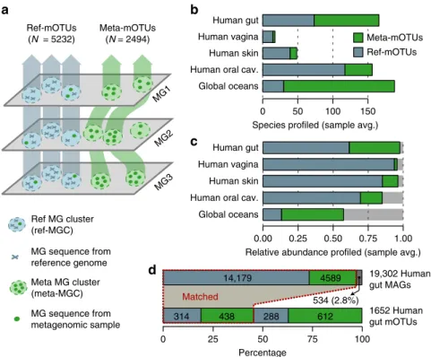
(>5 MGs per mOTU) as for ref-mOTUs (Fig.

1

a, Methods).

To evaluate the binning accuracy of meta-mOTUs, we assessed

individual MGCs in terms of taxonomic consistencies (Methods),

variations in abundance, prevalence and GC-content of individual

MGCs in comparison to ref-mOTUs (Supplementary Figure 2,

Methods). Overall, we found high agreement in all categories.

For example, at the species level, >97% (s.d.: ±1.5%) of

meta-mOTUs are expected to be completely consistent in their

taxo-nomic annotation (Supplementary Figure 2a), despite known

incongruencies between species name assignments and MG-based

sequence divergence

4

.

After quality control, the resulting 2494 meta-mOTUs,

together with the 5232 ref-mOTUs, comprise the updated mOTU

database. Compared to the previous version, these numbers

correspond to a 3-fold and 7-fold increase in known and

unknown species, respectively, that can now be profiled using

mOTUs2. Taxonomic ranks for each mOTU were assigned by a

last common ancestor-based consensus assignment

(Supplemen-tary Figure 3, Methods). Also, phylogenetic reconstruction shows

that meta-mOTUs were sampled from a broad taxonomic

distribution (Supplementary Figure 4), including from taxa that

were hypothesized to represent novel phyla

23

_{. Across all included}

biomes (four major human body sites and the ocean), the number

and fraction of unknown species (85%) were highest in ocean

water samples (Fig.

1

b), which is in congruence with previous

results

22

_{. Notably, even in presumably well-explored human gut}

samples, we found that more than half of the species still lacked

sequenced representatives in our reference genome database

13

(Fig.

1

b, c). A breakdown of mOTUs by biome showed that

ref-mOTUs are often detected in multiple biomes, while

meta-mOTUs tend to be more biome-specific (Supplementary

Figures 5a, b). As shown by rank-abundance analyses, we

find

meta-mOTUs to be well distributed across the range from

dominant to rare species (Supplementary Figure 6). Finally, the

MGCs that could not be binned were used to quantify the

cumulative abundance of organisms that are known to be present,

but not quantified as mOTUs (Methods). This fraction was

higher for the ocean than for samples from human body sites

(Fig.

1

c), which may be improved by increasing the number of

profiled ocean metagenomes in the future.

We next evaluated the sensitivity of mOTUs2 for unknown

species and assessed the resulting impact on relative abundance

estimations compared to other approaches. To accomplish this,

we analyzed the correspondence between mOTUs and

metagen-ome assembled genmetagen-omes (MAGs). MAGs involve binning

assembled metagenomic contigs by sequence composition and/

or read abundance variation as a strategy to detect and

genomically characterize organisms found in environmental

samples

24

_{. Thus, similar to meta-mOTUs, MAGs may include}

taxa that are not yet represented in genomic databases, and thus

provide a way to test if and how many environmental microbes

would be captured by mOTUs. More specifically, we

recon-structed MAGs from 4880 published human gut metagenomes

(Supplementary Data 2) and used 1845 MAGs identified in ocean

water samples as a subset of 8000 recently published MAGs

23

_.

Using these MAGs, we determined how many of them could be

assigned to previously known (ref-mOTUs) vs. unknown species

(meta-mOTUs) and evaluated the impact on relative abundance

estimations. We found that >97% of MAGs from human gut

samples were represented by mOTUs (Fig.

1

d). Among these,

76% could be matched to ref-mOTUs and the remainder to

meta-mOTUs. In addition, although the majority of the MAGs could

be assigned to mOTUs, they represented only 42% of all human

gut meta-mOTUs. For ocean water MAGs, 55% were represented

by mOTUs (19% of these matching ref-mOTUs), while MAGs

represented only 25% of ocean meta-mOTUs (Supplementary

Figure 7). Our results indicate that the most abundant organisms

in the human gut are already represented in public genome

databases, whereas a substantial additional fraction becomes

accessible through metagenomic data analysis. While assembly

opens possibilities for many additional analyses, higher sequence

coverage is required for the reconstruction of high-quality MAGs

than for mOTUs, explaining why meta-mOTUs capture many

more species. In the ocean, even some of the most abundant

species still appear to lack representative genomic

informa-tion (Supplementary Figure 7).

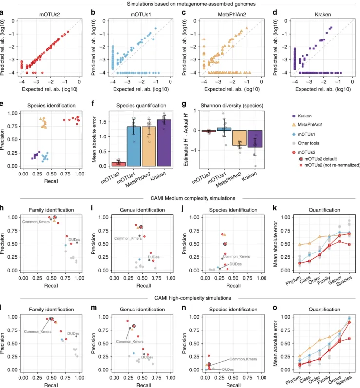
Next, we assessed the advantage of using a

reference-independent method for species quantification in microbial

communities. To this end, we compared mOTUs2 with two

popular reference-dependent approaches, as well as its original

version (mOTUs1

9

_{), using: (i) simulated metagenomes from}

human gut-associated MAGs (Supplementary Figures 8, 9 and

Methods), (ii) the Critical Assessment of Metagenome

Inter-pretation (CAMI) dataset

25

(Supplementary Figures 10, 11), and

(iii) the simulated metagenomes used to evaluate MetaPhlan2

7

_for

benchmarking (Fig.

2

; Supplementary Data 3, 4; Supplementary

Table 1). Our results based on simulated MAGs show that in

terms of precision, mOTUs2 and MetaPhlan2 outperformed

mOTUs1 and Kraken (Fig.

2

e). The fact that the

reference-dependent methods MetaPhlan2 and Kraken can only detect

genomes that are closely related to those present in current

reference databases was well reflected in a reduced sensitivity,

higher mean absolute error and deviations from expected

taxonomic diversity estimates (Fig.

2

e–g). Additional simulations

showed that relative abundance estimates may be highly

inaccurate when solely relying on reference genomes if unknown

species are present in medium to high abundance (Supplementary

Figures 9, 11). For the CAMI dataset, our results show that the

mOTUs2 profiler outperformed many other tools (Fig.

2

h–o;

Supplementary Figures 10, 11). More specifically, mOTUs2 not

only outperformed mOTUs1 at all taxonomic ranks, but also

other tools, including MetaPhlan2 above the genus level for

medium complexity simulations and above the species level for

high complexity samples (Fig.

2

k, o). We should note that in the

CAMI benchmark (and the OPAL evaluation tool

26

_{) profiled}

abundance data are re-normalized based on the detected taxa (see

0.00 0.25 0.50 0.75 1.00 0 50 100 150 Human gut Global oceans Human vagina Human skin Human oral cav.

Human gut

Global oceans Human vagina Human skin Human oral cav.

Meta-mOTUs Ref-mOTUs Ref MG cluster (ref-MGC) Meta MG cluster (meta-MGC) MG sequence from reference genome MG sequence from metagenomic sample

a

b

c

d

19,302 Human gut MAGs 0 25 50 75 100 Percentage Matched 1652 Human gut mOTUs 14,179 4589 534 (2.8%) 314 438 288 612 MG1 MG2 MG3 Ref-mOTUs (N = 5232) Meta-mOTUs (N = 2494)

Relative abundance profiled (sample avg.) Species profiled (sample avg.)

Fig. 1 Construction of marker gene-based OTUs (mOTUs) for metagenomic profiling. a Schematic illustration of the mOTUs concept (Methods). b The observed richness of ref-mOTUs (containing exclusively MG sequences from reference genomes; blue) and meta-mOTUs (containing only MG sequences from metagenomes; green) per biome, andc mean cumulative relative abundance of species profiled across 2481 metagenomic samples. d Correspondence between mOTUs and 19,302 metagenome assembled genomes (MAGs) from the human gut. While less than 3% of MAGs are not represented (dark grey bar), mOTUs allow for profiling of 900 species not captured by MAGs. Source data are provided as a Source Data file.

Estimated H ' -Actual H'

Shannon diversity (species)

Mean absolute error 0.00 0.25 0.50 0.75 1.00 0.00 0.25 0.50 0.75 1.00 Recall Family identification Family identification Genus identification Genus identification Precision

mOTUs1 MetaPhlAn2 Kraken

−4 −4 −3 −3 −2 −2 −1 −1 0 0 −4 −3 −2 −1 0

Expected rel. ab. (log10)

Species quantification Quantification Quantification Species identification Species identification Species identification Expected rel. ab. (log10)

−4 −3 −2 −1 0

Expected rel. ab. (log10)

−4 −3 −2 −1 0

Expected rel. ab. (log10)

Predicted rel. ab. (log10) −4 −3 −2 −1 0 Predicted rel. ab. (log10) −4 −3 −2 −1 0 Predicted rel. ab. (log10) −4 −3 −2 −1 0 Predicted rel. ab. (log10) mOTUs2 Common_Kmers DUDes 0.00 0.25 0.50 0.75 1.00 0.00 0.25 0.50 0.75 1.00 Recall 0.00 0.25 0.50 0.75 1.00 Recall 0.00 0.25 0.50 0.75 1.00 Recall 0.00 0.25 0.50 0.75 1.00 Recall 0.00 0.25 0.50 0.75 1.00 Recall Precision 0.00 0.25 0.50 0.75 1.00 Precision Common_Kmers DUDes 0.00 0.25 0.50 0.75 1.00 Precision 0.00 0.25 0.50 0.75 1.00 Precision 0.00 0.25 0.50 0.75 1.00 Precision 0.00 0.25 0.50 0.75 1.00 Recall 0.00 0.25 0.50 0.75 1.00 Precision 0.00 0.25 0.50 0.75 1.00 Common_Kmers DUDes _Mean absolute e rror 0.00 0.25 0.50 0.75 1.00 Mean absolute error Common_Kmers _DUDes Common_Kmers DUDes _{Common_Kmers} DUDes PhylumClassOrderFamilyGenusSpecies PhylumClassOrderFamilyGenusSpecies

a

b

c

e

f

g

d

h

i

j

k

l

m

n

o

Kraken MetaPhlAn2 mOTUs1 Other tools mOTUs2

mOTUs2 (not re-normalized) mOTUs2 default

MetaPhlAn2 Kraken mOTUs1

mOTUs2

Simulations based on metagenome-assembled genomes

CAMI Medium complexity simulations

CAMI high-complexity simulations

MetaPhlAn2 Kraken mOTUs1 mOTUs2 –1 0 1 0.0 0.5 1.0 1.5

Fig. 2 Evaluation of mOTU profiling on simulated samples. Benchmarks of quantification accuracy (a–g) on ten simulated metagenomic samples (Methods) containing MAGs with (n = 50) and MAGs without (n = 50) a representative reference genome sequence, (h–o) and the CAMI challenge datasets25_{.a–d A representative simulated metagenome (out of ten; Supplementary Figures 8, 9) analysed with four profilers. e Precision-recall}

plot, where each data point corresponds to one of the ten simulated samples. Mean absolute error (MAE, also referred to as L1 norm) (f) and differences of the Shannon diversity index (g) from the expected values (error bars in f and g show standard deviation). h–j Average precision-recall values over the two medium complexity samples and (l_{–n) average precision-recall values over the five high complexity samples of the CAMI dataset (see} also Supplementary Figure 10). Each precision-recall plot containsfive values for mOTUs2, which correspond to different sets of parameters: high precision (-l 140 -g 6), default (-l 100 -g 3), recall (-l 75 -g 3), high recall (-l 50 -g 2) and maximum recall (-l 30 -g 1), indicating the versatility of mOTUs2 in optimising precision or recall. In (k) and (o), mean absolute errors (MAE; referred to as L1-norm in CAMI) at different taxonomic ranks are shown for several tools. For mOTUs2, results for two options of calculating relative abundances are shown: one with relative abundances re-normalized based on detected taxa, which is enforced in the CAMI evaluation (but artificially deteriorates quantification accuracy), and one without this additional re-normalization (see main text and Supplementary Figure 11 for details). Data are provided in Supplementary Data 3, 4. Other taxonomic profilers (MetaPhyler, TIPP, Taxy-Pro, FOCUS, CLARK, Quickr) evaluated in CAMI25_{are denoted by grey dots. Source data are provided}

Supplementary Figure 11b). This re-normalisation procedure

penalises tools, such as mOTUs2, that can account for the relative

abundance of unknown taxa (Supplementary Figures 1, 11b).

This feature leads to improved quantification (hence, a

further reduction of the mean absolute error), in particular at

the species level (Fig.

2

k, o; Supplementary Figure 11a). Finally,

since Kraken was not included in the CAMI benchmark

25

_dataset,

we compared the performance of mOTUs2 to the results

reported for the evaluation of MetaPhlan2

7

_{, which included}

Kraken

6

_{. We}

_{find that mOTUs2 and MetaPhlan2 performed}

similarly, while both (and mOTUs1) outcompeted Kraken

(Supplementary Table 1).

Given that profiling unknown species in addition to those

represented in genome databases significantly improves relative

abundance estimates, we sought to assess potential impacts on

describing community structural properties. The total number

of detected species and their relative abundance distribution

determines the alpha diversity of a microbial community. This

parameter is of fundamental interest in microbial ecology

including in studies of gastrointestinal diseases

27

_{. As the}

quantitative breakdown of unknown species into mOTUs

provides more accurate estimates of relative species abundances,

measures for alpha diversity, such as the Shannon index (H’),

were expected to be more accurate for mOTU-based profiles

compared to reference-dependent approaches (based on

simula-tions, Fig.

2

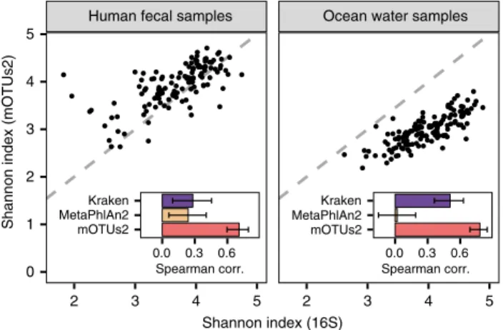
g). To test this further using real microbial

community

data,

we

compared

mOTUs2

to

reference-dependent methods against 16S rRNA gene-based approaches.

In two example data sets, one from a colorectal cancer study

21

(n

= 129) and one from an ocean ecosystem survey

22

_(n

_{= 139),}

we found mOTUs2 profiles to have higher correlations with

16S rRNA gene-based estimates of alpha diversity (Spearman

R

= 0.71, P < 0.0001 and R = 0.78, P < 0.0001, respectively) than

the reference-dependent methods (Fig.

3

and Supplementary

Figure 12).

We also assessed the performance of methods at estimating

how similar taxonomic compositions are between samples (beta

diversity). For this, we used data from healthy individuals who

donated samples from four different major body sites on multiple

sampling occasions

14

, so that composition similarities could be

compared

within

and

between

individuals.

Given

that

compositional differences are expected to be smaller within than

between individuals

14

, we tested in how many cases a sample

from one subject would be most similar to another sample from

the same individual (and body site) than from any other sample

in the set of >1200 samples tested. As a result, we found

that mOTUs2 performed similarly to the reference-dependent,

clade-specific gene-based method

7

_{, while both outperformed the}

whole genome-based method used by Kraken

6

(Supplementary

Figure 13).

Unbiased metatranscriptomic profiling using marker genes.

Although metagenomics data can be used for taxonomic profiling

of microbial communities, it does not allow determining whether

community members are physiologically active or not. Analogous

to DNA for metagenomics, metatranscriptomics refers to the

sequencing of reverse-transcribed RNA present in a microbial

community. Depending on environmental conditions, the

num-ber of transcripts per cell varies for most genes. An exception to

this are housekeeping genes that are expressed constitutively and

with low variability under different conditions. Thus, the

abun-dance of transcripts from such genes should strongly correlate

with the abundance of active cells in a community. As all ten

MGs are universal and involved in the highly conserved process

of translating mRNA to proteins, we hypothesized that

meta-transcriptomic abundances would serve as particularly good

proxies for relative cell abundances. To test this, we compared

mOTUs2 to reference-dependent methods that have been used in

recent metatranscriptomic studies

28, 29

_{or analysis workflows}

30

relating metatranscriptomic profiles to microbial abundance

and/or activity. More specifically, we correlated matching

meta-genome and metatranscriptome profiles from human stool

sam-ples

31

_{. At the species level (Fig.}

₄

_{a, Supplementary Figure 14),}

mOTUs2-based correlations were considerably higher (median

Spearman’s R = 0.76) than for reference-dependent methods

(R

= 0.37 and 0.45). Furthermore, we summarized mOTU

abundances at the class level and computed all pairwise distances

for all metagenomic and metatranscriptomic profiles to test for

each metagenomic profile whether the most similar

metatran-scriptomic profile matched the same sample. For mOTUs2,

this was the case for 92% of the samples compared to 78% and

64% for reference-dependent methods (Fig.

4

b, Supplementary

Figure 15).

MG-based SNV pro

filing for microbial population analyses.

Originally, the ten MGs were identified as a subset of candidate

phylogenetic marker genes deemed suitable for reconstructing

the tree of life

32

_{due to their universal occurrence and low}

rate of horizontal gene transfer

33

_{. These properties provided us}

with the opportunity to test how well single nucleotide variation

(SNV) profiles of microbial populations could be recapitulated

by the MGs comprising mOTUs as a compute-efficient

alter-native to using whole reference genome sequences. To this end,

we generated metagenomic SNV profiles

34

_{for sets of samples}

from different human body sites and ocean water using

ref-mOTUs and representative genome sequences as reference

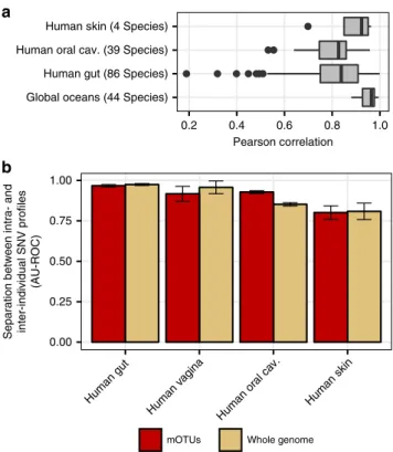
databases. Despite some differences between biomes (Fig.

5

a)

and a few species, we found overall that the distances of SNV

profiles using MGs were highly correlated (R > 0.8; Pearson) with

those obtained using whole genomes. For example, we

find

almost perfect correlations for ocean microbial species (median

R

= 0.96), and for most gut microbial species (median R = 0.84)

including those for which sub-species population structure was

recently identified

12,15,35

_{(Supplementary Figure 16).}

Having established the possibility of resolving mOTUs below

the species level, we addressed the question of how variable

Human fecal samples Ocean water samples

2 3 4 5 2 3 4 5 0 1 2 3 4 5 Shannon index (16S)

Shannon index (mOTUs2)

0.0 0.3 0.6 mOTUs2 MetaPhlAn2 Kraken 0.0 0.3 0.6 mOTUs2 MetaPhlAn2 Kraken Spearman corr. Spearman corr.

Fig. 3 Reference-extended mOTUs for microbial community diversity profiling. Shannon index was calculated based on 16S rRNA gene (16S) fragments (x-axis) and mOTUs (y-axis), respectively, for 129 human faecal samples (left) and 139 ocean water samples (right). Mean Spearman correlation of diversity estimates based on 16S and three metagenomic profiling tools (Kraken, MetaPhlAn2 and mOTUs2) are shown in the insets. Error bars delineate 95% con_{fidence intervals after bootstrapping. Source} data are provided as a Source Datafile.

microbial strains populations were over time in different human

body sites. Previously, microbial strain populations were shown

to display a high degree of individuality e.g., in the gut, skin, and

oral sites

11,36,37

_{. However, a comparative analysis of the degree}

of individuality of strain populations across different human

body-sites has not yet been performed. Using both ref-mOTUs

and meta-mOTUs, we compared strain population similarities

of body site samples collected in the HMP project

14,15

_{and found}

that stool and vaginal samples display the highest degree of

individuality, followed by oral and skin samples. Again, these

results were highly consistent with those obtained for reference

genomes (Fig.

5

b and Supplementary Figure 17).

Discussion

The original development of the mOTU profiler was driven by the

motivation to extend reference-dependent profiling of human gut

microbial species to uncharacterized taxa. As more environments

are subjected to metagenomic profiling, more data sets

are becoming available that can be used for approaches based

on binning genes by co-abundance analysis. With the inclusion of

new microbiomes, we found that some human body sites are very

well represented by available reference genomes (in particular skin

and vagina). In contrast, more than 50% of gut microbial species

still lack representative reference genomes (see also ref.

38

),

which may seem unexpected, but this estimate is in the same

range as reported for an independent approach

39

_{. This may in}

part be due to methodological improvements in the binning of

MGs into meta-mOTUs (Methods), increasing the number of

potentially uncharacterized species that can be profiled. In

addi-tion, we included not only more samples, but also data from a

number of disease-related studies (e.g., CRC, liver cirrhosis, type 2

diabetes) with large geographic distribution both contributing to

an extended diversity of species that were not profiled previously.

These may include species of particular relevance for

differ-entiating healthy from diseased states. Furthermore, our results

highlight the critical need to generate more reference genomes

for the ocean environment where we

find only 15% of species

to have a representative genome sequenced. Future efforts could

aim at extracting MGs from high-quality MAGs and single

amplified genome sequences to incorporate these into the mOTU

database.

Although metagenomics data can be used to profile the

abundance of microbial taxa in a given community, they do not

inform us as to whether they are also (transcriptionally) active.

To discern genomic potential from activity, the combined use

of metagenomics with metatranscriptomics profiling is becoming

increasingly popular. Here, we found that metatranscriptomic

abundances of mOTUs are highly correlated with metagenomic

abundances, which highlights the property of MGs as

con-stitutively expressed housekeeping genes across different

condi-tions. This suggests that mOTUs should be useful for normalizing

metatranscriptomics data for differential gene expression

ana-lyses. Other methods depending on genes that are conditionally

or variably expressed are demonstrably less suitable for this

approach and may also give the misleading impression that

many taxa are rare, but highly active, or abundant, but inactive or

dead (Supplementary Figure 15).

Spearman correlation 0.00 0.25 0.50 0.75 0.64 0.44 0.78 0.45 0.92 0.66 Average Verrucomicrobiae Negativicutes Methanobacteria Gammaproteobacteria Erysipelotrichia Deltaproteobacteria Coriobacteriia Clostridia Betaproteobacteria Bacteroidia Bacilli Actinobacteria Correct matches Kraken MetaPhlAn2 mOTUs2

a

b

0.66 0.58 0.60 −0.05 0.84 0.11 0.64 0.75 −0.05 0.91 0.19 0.15 0.88 0.25 0.21 0.16 0.37 0.52 0.44 0.58 0.73 0.45 0.36 0.44 0.90 0.64 0.86 0.42 0.59 0.67 0.80 0.73 0.87 0.87 0.16 0.42 1.1e–05 2.9e–11 2.9e–11 0.2 0.4 0.6 0.8 Spearman correlation Kraken MetaPhlAn2 mOTUs2

Fig. 4 Metatranscriptomic abundance profiling with mOTUs2. a Spearman correlation between matched metagenomic and metatranscriptomic pro_{files obtained from 36 faecal samples with Kraken, MetaPhlAn2 and} mOTUs2. mOTUs2 profiles (red) show significantly higher correlation than the other two methods (paired two-sided Wilcoxon test, boxplots show the median correlation as horizontal lines and interquartile ranges as boxes, whiskers extend at most 1.5 times the interquartile range).b The top-row represents the proportion of cases in which the distance (log-Euclidean) between metagenomic and metatranscriptomic pro_{files was smallest for} the same sample. Below is a taxonomic breakdown (12 most abundant classes) of correlations between metagenomic and metatranscriptomic profiles. For each class, the highest correlation value across the tested methods are shown in bold. Source data are provided as a Source Datafile.

Global oceans (44 Species) Human gut (86 Species) Human oral cav. (39 Species) Human skin (4 Species)

0.2 0.4 0.6 0.8 1.0

Pearson correlation

Separation between intra- and inter-individual SNV profiles

(AU-ROC)

mOTUs Whole genome

a

b

0.00 0.25 0.50 0.75 1.00 Human gut Human v agina Human or al ca v. Human skin

Fig. 5 Marker gene-based SNV profiles are comparable to those using whole genomes.a Pearson correlation coefficients for MG- and genome-based SNV profiles across species and biomes in the HMP (N = 2807) and ocean dataset (N = 139). Median correlations (Pearson’s r) are shown as horizontal lines and interquartile ranges as boxes. Whiskers extend at most 1.5 times the interquartile range.b Intra- and inter-individual distances of SNV profiles were compared using the area under the receiver operating characteristic curve (AU-ROC) to determine the degree of individuality of microbial strain populations for different human body sites (see also Supplementary Figure 17). Error bars delineate 95% con_{fidence intervals} after bootstrapping. Source data are provided as a Source Datafile.

The computation of metagenomic SNV profiles to study

microbial strain population differences is both resource and

time-consuming when using methods based on whole reference

gen-ome sequences

34,38

_{. We show that the use of mOTUs provides a}

fast and efficient alternative for profiling abundant species in

microbial communities. In addition to the improved efficiency,

mOTUs enable studying differences in strain populations of

species that currently lack a representative genome sequence. This

may be particularly relevant for disease-associated species and

biomes for which only few reference genomes are available. A

breakdown of intra-individual strain population similarity by

species also allows for distinguishing those with high specificity,

potentially under the control of the immune system, from those

that only transiently populate their host. Promising applications

of this approach could include testing the efficacy of

strain-retention after faecal microbiota transplantation

10

_{or studying}

dispersal patterns of microbial populations in the environment.

Methods

The mOTUs2 profiler. The mOTU profiler version 2 (mOTUs2) is a stand-alone, open source, computational tool that estimates the relative abundance of known as well as genomically uncharacterized microbial community members at the species level using metagenomic shotgun sequencing data. The taxonomic profiling method is based on ten universally occurring, protein coding, single-copy phylo-genetic marker genes (MGs), which were extracted from more than 25,000 refer-ence genomes13_{and more than 3100 metagenomic samples (Supplementary} Data 1; in total ca. 367,000 non-redundant MG sequences). The MGs were grouped into >7700 MG-based operational taxonomic units (mOTUs) that represent microbial species, many of which (ca. 30%) still lack sequenced reference genomes. In addition to (i) taxonomic profiling, the tool allows for (ii) basal transcriptional activity profiling of community members using metatranscriptomic data as well as (iii) determining proxies for strain population genomic distances based on single-nucleotide variations (SNVs) within the phylogenetic marker genes that comprise mOTUs.

Generation and annotation of the mOTUs2 database. The mOTUs2 profiler relies on a custom-built database of MG sequences extracted from reference gen-omes (ref-MGs) and from metagenomic samples (meta-MGs). The reference genomes were grouped into species-level clusters (specI clusters) and MG sequences from these reference genomes were grouped based on their specI affiliation into reference marker gene clusters (ref-MGCs). These ref-MGCs were augmented by MGs and the remaining MGs were clustered into meta-MGCs. MGCs of different MGs were subsequently grouped based on their specI affiliation or binned based on co-abundance analysis into reference genome-based mOTUs (ref-mOTUs) and metagenomic mOTUs (meta-mOTUs), respectively. The resulting mOTUs were quality-controlled, compiled into a sequence database for short-read mapping and taxonomically annotated. Regular updates of the of the mOTU database will be made available at:http://motu-tool.org.

Collection of MGs from reference genomes and metagenomes. The 25,038 reference genomes used for the mOTU database were downloaded from the pro-Genomes database13_{. Metagenomic data were downloaded from the Genbank} Sequence Read Archive (https://www.ncbi.nlm.nih.gov/sra) and the European Nucleotide Archive (https://www.ebi.ac.uk/ena) (accession numbers are listed in Supplementary Data 1). Most samples were obtained from human microbiome studies, including 1210 samples from different major human body sites (oral, skin, gut and vaginal14,15_{and 1693 further samples from various human gut} micro-biome studies16–21_{. In addition, we used 243 metagenomic samples from an ocean} microbiome study22_{. All samples were processed for marker gene identification}9_. Briefly, quality-controlled raw sequencing reads were subjected to metagenomic assembly and genes predicted on contiguous sequences longer than 500 base pairs (bp). MGs were subsequently extracted using the fetchMGs tool (available athttp:// motu-tool.org/fetchMG.html). In short, fetchMGs identifies MGs using HMM models built with HMMER3 (http://hmmer.org) applying a set of optimized cutoffs4,9_{, and extracts corresponding nucleotide sequences with the Seqtk tool.} With this workflow we extracted a set of 40 MGs (COG0012, COG0016, COG0018, COG0048, COG0049, COG0052, COG0080, COG0081, COG0085, COG0087, COG0088, COG0090, COG0091, COG0092, COG0093, COG0094, COG0096, COG0097, COG0098, COG0099, COG0100, COG0102, COG0103, COG0124, COG0172, COG0184, COG0185, COG0186, COG0197, COG0200, COG0201, COG0202, COG0215, COG0256, COG0495, COG0522, COG0525, COG0533, COG0541, COG0552)32,33_{from all 25,038 reference genomes. Not all of these} genes are currently suitable for metagenomic applications due to high rates of ambiguous mapping of short reads owing to highly conserved regions within MG sequences as well as lower assembly rates observed for some MGs4,9_{. Hence, a}

selected subset of ten MGs (COG0012, COG0016, COG0018, COG0172, COG0215, COG0495, COG0525, COG0533, COG0541, COG0552) was extracted from genes that were predicted in metagenomes as described above.

Grouping of MGs into ref-MGCs and meta-MGCs. Reference genomes were processed and clustered into specI clusters to build ref-MGCs4_{. To this end, we} calculated pairwise global nucleotide identities for all genome for each of the 40 MGs using vsearch (version v1.9.3)40_{. Genome-to-genome distances were} calcu-lated as the gene length-weighted arithmetic mean of the individual MG sequence distances. The resulting distance matrix was used as input for average linkage clustering using an optimized cutoff of 96.5% nucleotide identity4_{, resulting in} 5306 specI clusters. To assess the quality of grouping genomes into specI clusters, we tested whether the taxonomic annotations of the individual genomes provided by the NCBI were congruent (Supplementary Figure 18). More specifically, all specI clusters were annotated taxonomically in accordance to their member genomes. SpecI clusters were either homogeneous (all members had the same species-level annotation), heterogeneous (different species annotations found in the same cluster) or undetermined (clusters only containing genomes with non-binomial species names such as: Synechocystis sp. PCC 6803). We further evaluated how many NCBI species names occurred multiple times (in different clusters). Subse-quently, the ten MGs suited for metagenomics were extracted from the specI clusters resulting in over 51,000 ref-MGCs.

To enable the profiling of species that are not yet represented by reference genomes, we extracted MG sequences from metagenomic assemblies using the fetchMGs tool. For clustering, wefirst calculated all pairwise distances between MGs from ref-MGs and meta-MGs using vsearch (version v1.9.3)40_{and retained} alignments of at least 20 aligned bases. Then, we used open-reference clustering (employing the average linkage hierarchical clustering algorithm) to augment the pre-existing ref-MGCs with meta-MGs. The remaining meta-MGs sequences were clustered into meta-MGCs containing only meta-MGs.

Binning of MGCs into mOTUs. As the clustering of meta-MGs into meta-MGCs was performed independently for each of the ten MGs, it resulted in unbinned meta-MGCs (as opposed to the ref-MGCs, which were grouped into mOTUs based on their specI cluster affiliation). In order to bin MGCs into mOTUs (i.e., to link MGCs originating from the same species), we utilized the property that genes (and therefore, MGCs) from the same species are expected to co-vary in abundance across metagenomic samples41_{. Accordingly, we calculated the correlation between} pairwise MGC abundances across all samples for each biome. We optimized the correlation measure and prevalencefiltering (as a means against the spurious correlation between low-prevalence MGCs, see9_{) for each biome separately based} on the AU-ROC determined by cross-validating the grouping of ref-MGCs for which membership in the same specI clusters served as a ground truth. As a result, we defined the following biome-specific parameters: human gut - prevalence filter: five samples, Pearson correlation of log-transformed relative abundance; ocean - prevalencefilter: five samples, Pearson correlation of relative abundance; human oral cavity - prevalencefilter: 50 samples, Pearson correlation of relative abun-dance; human vagina - prevalencefilter: five samples, Pearson correlation of log transform relative abundance; human skin - prevalencefilter: ten samples, Spear-man correlation of log-transformed relative abundance. In order to combine the biome-specific correlations we transformed each of these into an FDR-calibrated association measure in such a way that for a given FDR value, the same association value was assigned. To obtain a single measure of association for each pair of MGCs, we computed the maximum of the FDR-calibrated association values across biomes.

For the actual binning, we used a slightly modified version of the greedy algorithm described in ref.9_{. As an initialization step, the ref-MGCs were grouped} according to their specI cluster affiliations. Then, meta-MGCs were progressively binned starting from the highest FDR-calibrated association values and decreasing until a cutoff value of 0.8 was reached. In this procedure, an MGC was added (binned) to an existing group (or another MGC to form a bin of size two) if this MG (among the ten possible ones) was not already present. Only groups with at least 6 MGCs were retained and defined as mOTUs, which resulted in 2494 meta-mOTUs (consisting only of meta-MGCs) and 5232 ref-meta-mOTUs (containing at least one ref-MGC and possibly additional meta-MGCs). MGCs that remained unbinned were grouped into a single unbinned group. Note that although specI clusters and ref-mOTUs are conceptually similar, there are two major differences: first, ref-mOTUs are composed of MGCs of at least six out of the ten different MGs used for metagenomics, while specI clusters represent genomes that are grouped based on distances calculated from up to 40 MGs; second, ref-mOTUs can, as described above, contain MGs and MGCs that were assembled from metagenomic samples.

To assess the expected taxonomic consistency of the binning strategy of meta-MGCs, a fraction of the ref-MGCs were treated in the same ways as meta-MGCs and their taxonomic affiliation (known from ref-mOTU membership) was only used afterwards to ascertain the error rate of the binning algorithm (Supplementary Figure 2a). Across all metagenomic samples used to construct the mOTUs, 1223 ref-mOTUs were detected and could be used for 100-fold resampled 5-fold cross-validation. We also assessed the agreement of the MGCs for each mOTU in terms of relative abundance and prevalence across metagenomic samples (Supplementary

Figures 2b,c). Relative abundance and prevalence showed higher agreement for meta-mOTUs than for ref-mOTUs. This was expected since the binning algorithm is directly influenced by these two parameters. We additionally evaluated the homogeneity of GC content among the MG sequences within each mOTU (Supplementary Figure 2d). meta-MGCs showed very homogeneous GC content, as expected for genes that originate from the same genome, but not for erroneously binned MG sequences.

Construction of the mOTUs2 mapping database. We compiled a sequence database against which short metagenomic reads can be aligned to quantify the abundance of MGCs and mOTUs. To construct a non-redundant mOTUs map-ping database, we removed identical MG sequences. MG sequences in the database were extended at the start and end of the gene by up to 100 nt, based on their genome or metagenomic assembly of origin, to reduce known mapping artifacts at gene boundaries. The resulting non-redundant database consists of the sequencefiles in FASTA format along with MGC and mOTU annotations, as well as the coordinates of the coding segments of the MG sequences. The sequencefiles were further indexed for searches with BWA42_{. For SNV calling, we constructed} an additional database that only consists of the centroid (medoid) sequence of every MGC so that SNVs can be identified with respect to one reference sequence per MGC.

Taxonomic annotation of meta-mOTUs. To assign taxonomic affiliations to meta-mOTUs, wefirst annotated each MG using Uniprot’s UniRef90 (https:// www.uniprot.org/uniref, release 2017_08) as a reference protein sequence data-base43_{, which was supplemented with a set of additional marine protein sequences} as described in44_{. Similarities between translated MG sequences and reference} database entries were computed using MMSEQS245_{with the following parameters:} search -a true -e 1E-5 --max-seqs 1000. Taxonomic affiliation was assigned using a weighted Lowest Common Ancestor (LCA) approach as follows: for each MG, all protein matches in the reference database with a value≥90% of the highest bitscore were kept. Then, outlier taxa were excluded by using a bitscore-weighted LCA annotation that covered at least 75% of the sum of all bitscores of each MG. Next, we transferred the annotation of the best-scoring MG member to each MGC and used the MGC annotations to assign a taxonomy to meta-mOTUs as follows: for each meta-mOTU and for each taxonomy rank, we required at least three MGCs to be annotated to consider the meta-mOTUs as annotated at this rank. Annotated meta-mOTUs were considered consistent if at least half of the MGC taxonomy annotations were in agreement.

Phylogenetic analysis of mOTUs. To explore the phylogeny of mOTUs (ref-mOTUs and meta-mOTUs), a reference tree was reconstructed by combining the phylogenetic signal of the ten sets of marker genes selected (Supplementary Figure 4). For this, all marker genes were translated into amino acid sequences and analyzed using ETE Toolkit v3.1. 146_{. In particular, the program ete-build was used} to run the following phylogenetic workflow: First, each set of marker proteins was independently aligned using ClustalOmega47_{. Next, alignment columns with} less than three aligned residues were removed. Finally, the ten individual MG alignments were concatenated and used to infer a maximum likelihood phyloge-netic tree using IQTree48_{and the LG model.}

The mOTUs2 profiling workflow. The mOTUs2 workflow for taxonomic pro-filing consists of three steps: alignment of metagenomic sequencing reads to MGs, estimation of read abundances for every marker gene cluster (MGC), and calcu-lation of mOTU abundances. As input, mOTUs2 expects the user to provide quality controlled sequencing reads. These are aligned to the MGs of the mOTU database using BWA (mem algorithm, default parameters)42_{. The resulting} alignments arefiltered and only those with at least 97% nucleotide identity are retained. Further, alignments arefiltered according to their lengths (default: 75 bp minimum alignment length; can be adjusted using the -l option).

Next, we compute the best alignment(s) for every insert (read pair) to the MGCs using BWA alignment scores. Inserts with a single highest scoring alignment areflagged as “unique alignments”, whereas inserts with multiple highest scoring alignments areflagged as “multiple alignments”. Subsequently, abundances for each MGC are calculated by summing up the number of all inserts flagged as unique alignments resulting in a unique alignment profile. Inserts flagged as multiple alignments are distributed among their best-scoring MGCs in accord with their respective abundances estimated based on the unique alignment profile. Thus, the final abundances are calculated as the sum of the unique abundance profiles and the distributed contributions of the inserts flagged as multiple alignments. In addition to these MGC insert counts, MGC base coverages are calculated byfirst summing up the total number of bases aligning to each MGC and then dividing by the respective gene lengths. Finally, the abundances of the mOTUs are calculated as the median of their respective MGC abundances (insert counts and base coverages). In order to reduce false positive results, we require a certain number of MGCs to be detected, that is to have metagenomic reads mapped to them (default: 3 MGs, -g option in mOTUs2). Although mOTUs2 is able to profile many organisms not yet represented by reference genomes, there are still around 25% of the MGCs that could not be

binned into mOTUs (see section 2.5). Reads mapping to those MGCs are assigned to a group labelled as“unbinned” (shown as “-1” in mOTU abundance profiles). The abundance of this group is calculated as the median of unbinned MGCs summed by COG.

Description of taxonomic pro_{filing outputs. The mOTUs2 profiler returns} multiple taxonomic profiles, since abundances based on read mappings can be calculated in different ways. One major distinction is the unit of counts. Either fragments such as inserts (or reads for single-pair sequencing) or mapped base-pairs can be counted. Counting the mapped base-base-pairs has the advantage that the mean base coverage can easily be computed by dividing the number of bases aligned to a certain gene by its corresponding length (mOTUs2 output -y option: “base.coverage”). Count based statistics are powerful for differential abundance testing (output -y option:“insert.raw_counts”). As the counts could in principle be non-integer numbers due to inserts mapping to multiple genes (see section 3.1), all counts are rounded to integers. For relative abundance-based estimates, gene-length normalizations are required to account for varying gene-lengths of MG sequences and varying numbers of MGCs present in each mOTU. To this end, we previously introduced“scaled counts” that retains most of the characteristics of insert counts. In this approach, coverages are calculated as described above and are then nor-malized to sum up to the number of inserts that align to MGCs (output -y option: “insert.scaled_counts”).

Single-nucleotide variant analysis with MGs. The mOTUs2 profiler has new functionality to compute metagenomic SNV profiles using the MGs comprising mOTUs as reference sequences. The resulting SNV profiles are highly correlated to those obtained by whole genome SNV profiling (see main text, Fig.5, Supple-mentary Figures 16, 17). The overall SNV calling pipeline starts by aligning metagenomic sequences to centroid sequences of MGCs (see above), before the resulting bamfiles are post-processed using metaSNV functions34_{. The mOTUs2} command map_snv maps the reads using BWA42_{and performs readfiltering in a} similar fashion as described for taxonomic profiling. For the SNV analyses, only insertsflagged as unique alignments are kept and the resulting sam file is sorted and converted into a bamfile. Using the snv_call command, the tool (i) computes base coverages, (ii) calls SNVs, (iii) generatesfiltered allele frequency tables, and (iv) calculates distances between strain populations.

These four steps are directly built upon metaSNV capabilities34_{, although the} procedure was adapted to mOTUs2 to facilitate its use with genes rather than genomes. Firstly, each bamfile is processed to compute per sample coverages for every reference sequence/mOTU, both vertical (average number of reads per position) and horizontal (percentage of the sequence covered at least once). SNVs are subsequently called using samtools mpileup49_{, followed by two post-processing} steps. This includes afiltering step, which was modified to include parallelized computing capabilities as well as the removal of padded regions in the allele frequency tables. Thefiltering parameters remain identical, with updated default values to account for the universal character of the genes considered: (-fb) minimal percentage of the sequence horizontally covered per sample and per mOTU (default= 80), (-fd) minimal average vertical coverage per sample and per mOTU (default= 5), (-fm) minimum number of samples meeting the listed criteria per mOTU (default= 2), (-fc) minimum vertical coverage per SNV position (default= 5), (-fp) minimum proportion of samples meeting the previous criterion at said position (default= 0.9). Finally, the filtered allele frequency tables are used to compute genetic distances between samples for each mOTU, Manhattan distances as well as major allele distances are used as the population genomic distance measure. For the latter, only allele frequency changes above 50% between the two samples are taken into account. The mOTU profiler uses parallelized computing capabilities for this step.

The output directory (-o) includes threefiles: two with the coverage information for each mOTU, both horizontal (*.cov.tabfile) and vertical (*.perc.tab file), and a logfile. Additionally, there are two directories: (i) per mOTU filtered allele frequencies of identified SNVs across samples (filtered-* directory) and (ii) per mOTU genetic distances between samples (distances-* directory), both Manhattan (mann.distfiles) and major allele (allele.dist files).

Benchmarking mOTUs2 against other tools. To evaluate its accuracy and robustness, we benchmarked mOTUs2 against two established tools for taxonomic profiling of metagenomic samples: MetaPhlAn27_{, which is based on clade-specific} marker genes, and Kraken50_{, which is based on exact alignments of genomic} k-mers. MetaPhlAn2 (version 2.6.0) was executed with default parameters. For Kraken-labelled analyses, we executed Kraken for read classification and calculated relative abundances with Bracken6_{. Kraken and Bracken were} installed as version 1.0.0 using conda. The Minikraken database (version mini-kraken_20171101_8GB_dustmasked) was downloaded fromhttps://ccb.jhu.edu/ software/kraken/. The Minibracken database was downloaded fromhttps://ccb.jhu. edu/software/bracken/on 1 February 2018. We executed kraken using paired-end and single-end data using default parameters. Abundance estimation with Bracken was performed with the following parameters: -k minikraken_8GB_75mers_distrib. txt -l S -o result.abundance.bracken.

Comparison of mOTUs with metagenome-assembled genomes. We further validated the mOTUs using metagenome-assembled genomes (MAGs) recon-structed from different environments. For this purpose, wefirst extracted 4880 metagenomic sequencing runs from human gut samples available from the Eur-opean Nucleotide Archive (accession numbers are listed in Supplementary Data 2). Raw reads from each run were assembled using metaSPAdes v3.10.051_and sub-sequently binned with MetaBAT2 (v2.12.1)52_{with a minimum contig length} threshold of 2000 bp. Sequencing coverage required for binning was inferred by mapping the raw reads back to the assemblies using BWA v0.7.1642_{and then} retrieving the percentage of mapped read bases with samtools v1.549_{and the} jgi_summarize_bam_contig_depths function from MetaBAT2. Quality scores (QS) of each metagenome-assembled genome (MAG) were estimated with CheckM v1.0.753_{, calculated as the level of completeness - 5 x contamination, as previously} described23_{. Good-quality MAGs (QS > 50) were kept for subsequent downstream} analyses. MAGs from marine samples (Ocean MAGs) were obtained as a subset of about 8000 MAGs, which are described in a recent publication23_{. In order to} identify ocean-associated MAGs, wefirst searched for the keywords: ocean, marine, baltic sea and north sea to extract entries in Supplementary Table 1 of23_{and found} 400 samples matching these keywords. From these samples, we selected 1845 MAGs (from Supplementary Data 2) that were reconstructed from these metagenomes.

Correspondence between MAGs and mOTUs was established using the following procedure:first, we extracted the ten MGs from the MAGs using fetchMGs (see above), obtaining a set of MAGs. Second, we aligned the MG-MAGs to the MG database of the mOTUs using vsearch -usearch_global (parameters: --id 0.96 --minqt 0.7). Finally, we evaluated the congruency of the MG-MAGs to mOTU matches. For this, wefirst checked if at least three MG-MAGs could be assigned to a mOTU (by mapping to a MGC that is part of a mOTU). If this was not the case the MAG was annotated as“unassigned/-1”. Next, we removed all alignments to MGCs not assigned to mOTUs and assigned a MAG to a mOTU if >50% of the MG-MAGs were consistently matched to the same mOTU. Otherwise (if no majority mOTU was found) the MAG is annotated as “inconsistent”.

Benchmarking mOTUs2 using simulated metagenomes. To be able to assess taxonomic quantification accuracy, ten human gut metagenomic samples were simulated using 15,102 Human gut MAGs: a subset of the 19,302 MAGs described before, excluding the MAGs created from samples used to construct the mOTU database (Supplementary Figure 8). MAGs with an ANI > 96.5% were de-replicated to have one representative MAG per species (cut-off according to ref.4_{). The ANI} was calculated with the fastANI tool [https://github.com/ParBLiSS/FastANI]. The corresponding fastqfiles (as well as the simulated abundance data) are available at:http://motu-tool.org/download.html. Metagenomic read data were simulated using BEAR54_{:first, we generated 100 M inserts (2 × 100 M paired-end reads of} 150 nt length) with 350 nt insert distance (standard deviation: 30) using gen-erate_reads.py. Second, trim_reads.pl with default parameters was used to add the quality scores, introduce errors and shorten the reads. Every sample was simulated based on mOTUs2 profiled relative abundances from ten real samples. For each simulated sample, we randomly selected 50 MAGs with a representative reference genome sequence in the superset of the Kraken, MetaPhlAn2, or ref-mOTU databases and 50 additional MAGs sampled from those that lacked any reference database representation (which does not preclude these MAGs to map to meta-mOTUs).

The benchmark was performed by evaluating precision-recall plots of the simulated metagenomes based on the number of true positives (TP) false positives (FP) representing species that are predicted but not present in the real sample, and false negatives (FN) representing species that are missed by the profiler. Precision is calculated as TP/(TP+ FP) and recall as TP/(TP + FN). Next we evaluated the mean absolute error (MAE) defined as the average absolute difference between estimated relative abundances and relative abundances simulated as ground truth. Finally we evaluated the accuracy of alpha diversity estimates using the difference between predicted and actual Shannon index (abbreviated as H’).

Benchmarking mOTUs2 using the CAMI framework. We further evaluated mOTUs2 in the CAMI framework25_{, which includes eight simulated samples} (one low complexity, two medium complexity andfive high complexity) for which the ground truth is available. Within thefirst CAMI community challenge, ten metagenomic profiling tools including MetaPhlAn2 and mOTUs1 were already benchmarked on these data sets. To comparatively assess the performance of mOTUs2 in this context, we converted its output to CAMI/Bioboxes format (-C option in the mOTUs2 profiler) and used OPAL 0.2.926_{(developed by the same} authors as CAMI) for consistency of performance assessments. Using precision-recall plots we evaluated mOTUs2 employingfive different parameter sets: high precision (-l 140 -g 6 -C precision), default (-l 100 -g 3 -C precision), recall (-l 75 -g 3 -C recall), high recall (-l 50 -g 2 -C recall) and maximum recall (-l 30 -g 1 -C recall). Hence mOTUs2 are represented byfive red dots in the precision-recall plots, demonstrating that it can be tuned to obtain a range of precision-recall trade-offs. The evaluation of the mean absolute error (MAE), which it is called L1 norm in the CAMI paper, was also obtained with OPAL. By default, OPAL re-normalises the relative abundances of the gold standard and the profiling result to each sum to

1 before calculating the MAE, which apparently substantially deteriorates the quantification accuracy of mOTUs2 (see Supplementary Figure 11b). For this reason, we included both re-normalised and relative abundances without any post-processing in our evaluation for mOTUs2. This aims for maximum transparency in the comparison to the other tools, which could only be evaluated with the re-normalised version (but could theoretically also benefit from an evaluation of non-normalised relative abundances).

Determining environmental specificity of mOTUs. To determine the environ-mental specificity of the mOTUs, we used the set of >3100 metagenomes (Sup-plementary Data 1) to assess the environmental specificity of all meta-mOTUs and the subset of ref-mOTUs that are present in these samples (Supplementary Fig-ure 5a). To this end, we generated mOTUs2 profiles of these samples with default settings and removed samples with less than 500 scaled insert counts. Based on the resulting profiles (https://motu-tool.org/data/All_2481_at_least_500.motu.nr. out.20180307.tsv), we classified a mOTU to be present in a specific environment

if it was detected in more than three samples from that environment.

Analysis of community structure. We assessed correlations of the Shannon index calculated based on 16S rRNA gene-based analyses and three metagenomic pro-filing tools (mOTUs2, MetaPhlAn2 and Kraken). For this we used data from two different biomes: metagenomes generated from stool samples of a colorectal cancer (CRC) study21_{and metagenomes from seawater samples of the Tara Oceans} expedition22_{. For the CRC study, amplicon sequencing data of the V4 region of the} 16S rRNA were downloaded from the European Nucleotide Archive (ENA) database (http://www.ebi.ac.uk/ena): accession number ERP005534. For the ocean water samples, 16S rRNA gene containing fragments were extracted from meta-genomic sequencing reads (miTAGs55_{). To ensure comparability between the data} sets, we extracted thefirst 100 bp from each miTAG sequence starting from the V4 primer sequence.

Ribosomal RNA data were initially processed using USEARCH56_(version 9.2.64) as follows: paired-end reads were merged and quality-filtered using the fastq_mergepairs command with default settings. Merged reads werefiltered using the fastq_filter command (-fastq_maxee 0.1). Sequences were de-replicated using the fastx_uniques command, singletons were excluded and the remaining unique sequences were clustered into operational taxonomic units (OTUs) at 97% with chimera removal using the cluster_otus command. Finally, OTU abundances for each sample were determined using the usearch_global command (-strand both; -id 0.97). The OTU abundance tables were downsampled to the minimum number of reads per sample (CRC: 40,805 reads, TARA: 1494 reads) to normalize for uneven sequencing depths using the R function rarefy within the vegan package57_. The Shannon index of diversity was computed for each sample and all methods (16S rRNA gene-based and metagenomic method-based) using the R function diversity of the vegan package. In order to obtain a 95% confidence interval we used bootstrapping (n= 100,000) by resampling pairs of Shannon index values. The confidence intervals reflect the 2.5 and 97.5 percentile of the bootstrapped samples.

Between sample distances were determined using human body site samples for which more than one time point was available for the same individual. More specifically, for each body site, we compared community compositional distances between samples from the same individual (intra-individual) to distances between this and other individuals (inter-individual). Canberra and Bray-Curtis distances were computed with the vegdist R function of the vegan package and the log-Euclidean distance was computed as the log-Euclidean distance of the log-transformed relative abundances after the addition of a pseudocount smaller than the smallest non-zero value. For each of the three distances and each sample, we identified the most similar sample (i.e. the one with the minimum distance value) and determined the proportion of cases in which both samples belonged to the same individual.

Analysis of metatranscriptomes. To demonstrate the use of mOTUs2 to assess basal transcriptional activity of microbial community members, we used a dataset from 36 samples for which metagenomic and metatranscriptomic sequencing data are available31_{. Each sample (36 metagenomes and 36 metatranscriptomes) was} subjected to profiling using mOTUs2, Kraken/Bracken and MetaPhlAn2. All resulting profiles were transformed to relative abundances, and log-transformed after adding a small pseudocount. After that, Spearman correlations between corresponding metagenomic and metatranscriptomic profiles generated from the same sample were calculated and compared between profiling methods (Fig.4a and Supplementary Figure 11). We moreover evaluated how well species abundance estimates correlated between metagenomic and metatranscriptomic profiles for the twelve most abundant taxa at the class level. Class level information for mOTUs and MetaPhlAn2 was available as part of the profiler output. Class level annota-tions for Kraken were obtained using NCBI taxonomy identifiers.

Comparison of SNV profiles from MGs and whole genomes. To assess the comparability of SNV profiles generated with mOTUs2 and whole genomes, we used samples from 2807 human microbiome samples14,15_{and 139} prokaryote-enriched metagenomes from the Tara Oceans project22_{. Metagenomic reads were} mapped to the mOTUs centroid database using the mOTUs2 command map_snv