Studying the Biomechanics of Total Knee Replacement
by
Ephrat Most
BSE Biomedical Engineering The University of Iowa, 1998
Submitted to the Department of Mechanical Engineering in Partial Fulfillment of the Requirements for the Degree of
Master of Science in Mechanical Engineering at the
MASSACHUSETTS INSTITUTE OF TECHNOLOGY June 2000
* 2000 Massachusetts Institute of Technology All rights reserved
/I
Author...
..f ...1-epartment of Mechanical Engineering
May 19, 2000
Certified by...
...Guoan Li
Assistant Profess r of Orthopedic Surgery/Bioengineering
larvard Medical School
Thesis Supervisor
Certified by.... ...
Derek Rowell
ProfeQar of Mechanical Engineering
T1nc Supervisor
A ccepted by ... ...
Ain A. Sonin Chairman, Department Committee on Graduate Students
MASSACHUSETTS INSTITUTE OF TECHNOLOGY
SEP 2 0
2000
Development of a 6-DOF Robotic Test System for Studying the
Biomechanics of Total Knee Replacement
by
Ephrat Most
Submitted to the Department of Mechanical Engineering in partial fulfillment of the requirements for the degree of
Master of Science in Mechanical Engineering
Abstract
A robotic-based joint testing system for studying the biomechanics of Total Knee Arthroplasty (TKA) was developed in this project. The system is composed of a 6 Degree-of-Freedom (DOF) robotic manipulator (Kawasaki UZ150*) and a 6-DOF universal force-moment sensor (JR3*). This testing system offers the ability to operate with force and displacement controls and is capable of characterizing the in-vitro kinematics and the in-situ forces in tissue components of the human knee. In a knee test, the femur is rigidly fixed on a pedestal while the tibia is rigidly mounted to the robot arm through the load cell. This robotic system determines the kinematics response of the knee under various external-loading conditions. The kinematics data can then be reproduced on the knee specimen. Upon simulation of knee motion, forces and displacements are evaluated from the load cell and the robot, respectively. Various TKA designs can be tested on the same specimen where the native knee is used as the reference for the evaluation of the biomechanical response of the TKA. The system could be further modified to determine optimal designs of various artificial joint replacements, using normal joint biomechanics as an objective function.
Thesis Supervisor: Guoan Li
Title: Assistant Professor of Orthopedic Surgery/Bioengineering, Harvard Medical School
Thesis Supervisor: Derek Rowell
To my parents:
Anyone who has never made a mistake has never tried anything new. -Albert Einstein
Acknowledgments
These past two years have been more than astonishing. I can clearly remember my first day at MIT. I was overwhelmed! Everything had a number and everyone referred to things as a number. It took me at least an hour to find building 1 (Mechanical Engineering office). At that time, it seemed reasonable to assume that building 1 is right next door to building 2, but it is not. I want to thank the people that helped me in my early days at MIT to the present. I want to single out a few special people.
First and foremost, I want to thank my advisors: Drs. Guoan Li, Derek Rowell, Harry Rubash, and James Herndon. It has been an honor and a privilege to work with such knowledgeable and experienced faculty. I especially want to thank Dr. Li who spent hours and hours patiently teaching me step-by-step the secrets of mechanical engineering and biomechanics. Dr. Li, you have been more than a mentor to me. Your knowledge, motivation, encouragement, and advice will be a role model in my career. I admire your patience and guidance even when I fell short of your expectations. I express my gratitude to Dr. Rowell for guiding me through my MIT experience, offering insight in system development, providing me with thesis guidance, and allowing me to simply stop by his office to tell him what is on my mind. Drs. Rubash and Herndon, I want to thank you both for allowing me to participate in this research. This is a very exciting field and it is my honor to work with you. Dr. Rubash, I cannot thank you enough for always finding time for me and my husband in your extremely busy schedule.
This work could not be done without the assistance of many other people. Leslie Regan, Joan Kravit, Bridget Riley, and Lori Humphrey; I could not have done it without
you! Thank you for all your help and guidance throughout these past two years. You have a special place in my heart (and in my teeth from all the candy that you provided me).
I thank the members of the Orthopedic Biomechanics Laboratory (OBL), past and
present, who have been there academically as well as socially. I thank each and every one of you for helping me when needed, for keeping me on my toes when I did not clean the tools, and for simply being there as friends. I am proud to be a member of the OBL! I deeply thank my lab partner, Lou DeFrate, for his energetic spirit and keen insights.
I would like to thank Maria Apreleva, Jennifer Copper, and Melissa Pierre who
had taken time to review this work and offer comments to improve its presentation. None of the TKA surgeries would have been possible without the cooperation and talent of Erik Ottorberg.
Part of my research involved testing of human cadavers. I want to thank the donors and their families for believing in improving the human conditions. Your generosity has been a tremendous contribution to knee biomechanics research.
I wish to thank a pioneer in the field of Musculoskeletal Biomechanics research,
Dr. Savio L-Y. Woo. Dr. Woo gave me the opportunity as an undergraduate student to take part in the MSRC summer internship research program. This was a real turning point in my academic career.
I express my thanks to two more people who had a tremendous influence on my
educational career: Drs. Vijay Goel and Lars Gilbertson who believed in me from the beginning.
Last but not least, I want to thank my family for all their support and sacrifices throughout the years. From the bottom of my heart I thank my mother, Ruth Most, for giving me the best I can get, often, more than I deserved. To my sisters, Liora (Lulu) and Ayala (Ayal) for helping mom when I was away and keeping me up-to-date with all the gossip over in Israel. To my husband, Sheldon: there are not enough words and space to express my thanks to you. You have been the light of my life. I could not have done it without you!
I remember with love, the first engineer in my life, my father Nathaniel Most
('"0. I walk in your shoes.
This work was funded by the National Science Foundation (NSF). TKA components were generously provided by Zimmer.
Contents
CHAPTER 1: INTRODUCTION... 15
1.1 M otivations and O bjectives ... 15
1.2 O rg an ization ... . . 19
CHAPTER 2: ANATOMY AND BIOMECHANICS OF THE HUMAN KNEE ... 20
2.1 K nee A natom y ... 20
2.1.1 T he L igam ents ... 2 1 2.1.2 T he M uscles ... . 23
2 .1.3 T he P atella ... . 24
2.1.4 T he M enisci ... 25
2.2 Current Status of Knee Joint Biomechanics ... 26
2.2.1 Biomechanics of the Human Knee Joint... 26
2.2.2 Biomechanics of Total Joint Replacement ... 29
CHAPTER 3: ROBOTIC TESTING SYSTEM FOR TKA BIOMECHANICS... 32
3.1 Displacement Control Device: Robot Manipulator ... 33
3.1.1 G eneral D escription ... 33
3.1.2 Communication with Personal Computer (PC) ... 34
3.2 Force Control Device: JR3 Universal Force/Moment Sensor ... 35
3.2.1 G eneral D escription ... 35
3.2.2 JR3 DSP Based Force Sensor Receiver Card ... 37
3.2.3 System Set-up: Force and Moment Measurements ... 37
3.2.5 Load Cell Calibration... 39
3.2.6 Load Cell Tare Load: The Effect of Gravity ... 41
3.3 D igitization System ... 43
CHAPTER 4: FORCE AND DISPLACEMENT CONTROL OF THE TEST SYSTEM45 4.1 General Description ... 45
4.1.1 Experimental Set-up... 45
4.1.2 Coordinate System Development ... 47
4.1.3 Knee-Load Cell-Digitizer Relationship ... 48
4.1.4 Robot-Knee-Load Cell Relationship... 51
4.2 Force Control Algorithm... 53
4.2.1 Use of Broyden's Method in the Control Algorithm... 54
4.2.2 Application of Broyden's Method in Finding the Neutral Path of a Human K n ee Jo in t ... 5 6 4.3 Displacement Control Mode ... 57
4.4 Application of the System for Measuring Ligament Force. ... 58
4.5 Significance of the System... 59
CHAPTER 5: DETERMINATION OF TKA KINEMATICS USING THE ROBOTIC S Y S T E M ... 6 0 5.1 Basis for Interpretation ... 61
5.2 T ranslation D ata... 62
5.3 R otation D ata ... . 64
5.4 Analysis and Conclusions... 66
A. 1 Position Vector and Rotation M atrix ... 68
A .2 E uler A ngles... . . 70
APPENDIX B: ROBOT PC COMMUNICATION... 74
B.1 AS Code for Sending Robot Location to PC ... 74
B.2 VB Code for Receiving Robot Location from PC... 74
B.3 AS Code for Receiving Robot Location from PC ... 75
B.4 VB Code for Sending Robot Location to C Controller... 76
APPENDIX C: JR3 DSP DATA LOCATION... 78
APPENDIX D: LOAD CELL TARE LOAD - VB CODE... 79
APPENDIX E: VB CODE: COORDINATE SYSTEM ESTABLISHMENT ... 81
APPENDIX F: BROYDEN'S METHOD ... 86
List of Figures
Figure 1.1: Lateral view of right knee after TKA... 16
Figure 2.1: Anterior view of a right knee. ... 21
Figure 2.2: The major muscles of the knee joint. ... 23
Figure 2.3: Lateral and anterior view of patella and patella tendon. ... 24
Figure 2.4: Anterior view of left knee outlining the medial and lateral menisci... 25
Figure 2.5: The effect of menisci on contact stresses:... 26
Figure 2.6: Posterior cruciate retaining TKA (right knee)... 30
Figure 2.7: Posterior cruciate substitution TKA (right knee). ... 30
Figure 3.1: The components of the robotic system:... 34
Figure 3.2: Communication protocol... 35
Figure 3.3: Address selection for the ISA bus receiver. ... 37
Figure 3.4: Forces and moments drifting behavior of the JR3 during 50 hours of o p eratio n . ... 4 0 Figure 3.5: Force calibration in the x and y directions. ... 40
Figure 3.6: Force (z direction) and moment (around z) calibration... 40
Figure 3.7: Load cell - fixture assembly. ... 41 Figure 3.8: Force in the x direction and moment around the x axis plotted for before and after tare lo ad . ... 4 3 Figure 3.9: Force in the y direction and moment around the y axis plotted for before and after tare lo ad . ... 4 3
Figure 3.10: Force in the z direction and moment around the z axis plotted for before and after tare lo ad . ... 4 3
Figure 3.11: M icroScribe parts and features... 44
Figure 4.1: Set-up of the robotic testing system ... 46
Figure 4.2: Tibia and femur coordinate system (CS) configuration: ... 47
Figure 4.3: Coordinate system determination for load cell and knee. ... 48
Figure 4.4: Schematic diagram of digitizer, load cell, and knee kinematics. ... 49
Figure 4.5: Graphic representation of the four coordinate systems... 52
Figure 4.6: Flow chart describing neutral path (NP) determination. ... 57
Figure 5.1: Knee coordinate system establishment; A. Knee at full extension, B. Knee after a given translation and a rotation... 61
Figure 5.2: Tibial translation with-respect-to femur CS in the X-direction (left knee).... 62
Figure 5.3: Tibial translation with-respect-to femur CS in the X-direction (right knee).. 62
Figure 5.4: Tibial translation with-respect-to femur CS in the Y-direction (left knee).... 63
Figure 5.5: Tibial translation with-respect-to femur CS in the Y-direction (right knee).. 63
Figure 5.6: Tibial translation with-respect-to femur CS in the Z-direction (left knee). ... 63
Figure 5.7: Tibial translation with-respect-to femur CS in the Z-direction (right knee).. 64
Figure 5.8: Tibial rotation with-respect-to X-axis of femur CS (left knee)... 64
Figure 5.9: Tibial rotation with-respect-to X-axis of femur CS (right knee)... 65
Figure 5.10: Tibial rotation with-respect-to Z-axis of femur CS (left knee). ... 65
Figure 5.11: Tibial rotation with-respect-to Z-axis of femur CS (right knee)... 65
Figure A .1: Position vector description ... 69
Figure A.3: Rotation about the Z-axis of a reference frame... 70
List of Tables
Table 3.1: UZ150 selected specification... 34
Table 3.2: JR3 sensor specific information... 38
Table 3.3: MiscroScribe-3DX selected specification. ... 44
Table 4.1: Coordinate system calculations for load cell and knee... 48
Table 4.2: Variables description. ... 49
Table 4.3: Variables summary. ... 52
Chapter 1
INTRODUCTION
1.1
Motivations and Objectives
Human knee joints are subjected to a wide range of forces during daily activities. These forces can be several times body weight for activities such as climbing stairs or rising up from a chair and can be as high as 10 to 20 times body weight for activities such as jumping or running. It is remarkable that the human joint can undergo millions of cycles under such high forces. However, there are many observations of human joint degeneration that eventually lead to surgical intervention. Joint degeneration is poorly understood, but there is no doubt that these high forces contribute to such a process [1-3].
Common symptoms of joint degeneration are reduced joint flexibility, development of bony spurs, joint pain, and swelling of the joint [4]. Osteoarthritis (OA) is one of the major degenerative joint diseases that develop in joints that are injured by repeated overuse in the performance of a particular activity or from carrying excess bodyweight. OA is frequently associated with aging due to general wear and tear in the joint. People with severe OA have problems performing even the simplest daily activities such as walking or getting up of a chair. An estimated 16 million Americans are
afflicted with OA. About 65% of the people with OA are over the age of 65. More men than women under the age of 45 have OA, but twice as many women as men over the age of 65 experience these conditions.
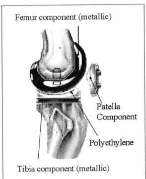
Total knee arthroplasty (TKA) has been a popular surgical procedure to treat people with severe degenerative joint disorder such as OA. This surgery is also performed to replace a badly fractured knee and when previous joint replacements have failed. The femoral component of a TKA is usually made of an alloy containing chromium, cobalt and molybdenum that are nearly inert in the body. The tibial component is often made of titanium that is lighter, stronger and leaves more space for the plastic bearing surfaces. The plastic is ultra high molecular weight polyethylene (UHMWPE), chemically similar to ordinary polythene but immensely hard and very
smooth (Figure 1.1) [84].
Femur component (metallic)
Patella Component
Polyethylene Tibia component (metallic)
In 1994, there were 230,342 TKA surgeries performed in the United States; 211,872 primary TKAs and 18,470 revisions [5]. Further, in 1997, the number of
inpatient procedures for arthroplasty and knee replacement increased to 338,000 [National Center for Health Statistics, National Hospital Discharge Survey, 1997]. TKA implants do not last indefinitely in the joint. The main mechanisms for TKA failure are loosening of the prosthesis from the bone, joint infection, polyethylene wear, component instability, poor range of motion, bone fracture, and patella complications. The joint may need to be changed but the second operation, which is more difficult than the first, may not be as successful and the knee may need to be stiffened [6-7].
Even though TKA is a popular procedure, the exact mechanisms that play a role in its success or failure are unknown. It is unclear about the exact role of the ligaments, patella, patella tendon, and muscle loading on both the kinematics (motion) as well as the kinetics (forces) of the knee after TKA. Limited information is available regarding both magnitude and location of the contact stresses within the artificial knee joint.
One of the most controversial issues regarding TKA is the role of the posterior cruciate ligament (PCL). Two schools of thoughts regarding the PCL contribution to TKA outcome can be found in the literature. Some researchers found that the PCL plays an important role in the restoration of normal knee function post TKA. Others reported that the PCL might contribute to complications after TKA. PCL retention has been advocated for its effect on keeping the femoral component rolling motion on the tibial plateau, and reducing tibial shear forces [8-12]. Others demonstrated that the PCL does not always cause posterior roll back of the femur in squatting, which might accelerate polyethylene liner wear on TKA [13]. Further, inadequate PCL tension may cause
abnormal kinematics following TKA. Inconsistent results regarding the surface strain of the PCL have been reported in the literature [14, 15]. In spite of extensive research the biomechanical role of the PCL in TKA remains unclear. Additional information (e.g. the constraint forces of the PCL) is needed for a more objective rather than subjective TKA. A method / system for quantitatively evaluating the mechanisms involved with TKA is
desired.
The primary objective of this work is to develop a non-contact experimental system for the quantification of PCL tension and tibio-femoral joint forces of the knee under physiological loads. The system is composed of a 6 degree-of-freedom (DOF) robotic manipulator and a 6 DOF load cell. This system determines knee joint motion under simulated muscle loads and measures ligament forces using the principle of superposition instead of attaching a sensor onto the target ligament. Using this system, it is possible to study the role of the PCL on TKA and to quantify the contact forces at the medial and lateral sides of the knee pre- and post- operatively for a variety of knee joint replacement implants. This information is important for joint stability and for the analysis of polyethylene wear. Key advantages of this system are repeatability, the non-contact measurements, and the capability to limit intra-specimen variation by performing multiple tests on the same knee specimen (intact knee, knee after various surgical modification, etc.).
1.2
Organization
This dissertation reports the development of a 6-DOF robotic system for studying the biomechanics of total knee joint replacement. The central focus is on the development of the system, its uniqueness and its future applications.
The text is organized sequentially. Chapter 2 contains a review of the anatomy and the biomechanics of the human knee. In addition, a literature review of relevant work both on the native knee as well as the TKA knee is presented. Chapter 3 reports a description for each of the components that make up the robotic testing system. The robotic system has both position and force control capabilities. In Chapter 4, the reader can find a description of how the system works. The final chapter presents the overall results of this project as well as suggestions for future directions of this project.
Chapter 2
ANATOMY AND BIOMECHANICS OF
THE HUMAN KNEE
In order to provide the fundamental background of this project, this chapter presents basic information in two areas. First, a detailed description of human knee anatomy is presented. Second, a literature review on knee joint biomechanics is presented.
2.1
Knee Anatomy
The knee is perhaps one of the most complicated joint in the human body. Mechanically, the two main functions of the knee are stability and mobility. The knee transmits loads, participates in motion, aids in conservation of momentum, and provides a force couple for activities involving the leg. Its articulating surfaces are frequently exposed to contact stresses and strains. The knee is a three-component structure (femur, tibia, and patella
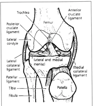
-Figure 2.1) that not only sustains high forces but also is located between the body's two largest lever arms. Therefore, it is susceptible to injuries and chronic diseases such as ligament rupture, meniscal tear, dislocations, arthritis, etc. Understanding of knee joint kinematics and tissue forces in response to external loads is crucial in the diagnosis of
joint disorders resulting from either an injury or a disease. Moreover, comprehensive knowledge of knee function plays an important role in the design of prosthetic devices as well as post-operative rehabilitation. In the following sections, the main components of the knee joint are described.
Trochlea Anterior cr cate ligament Posterior Femur cruciate ligament -Lateral condyle
La tera 1 Lateral and media
-ccoy\lateral m ns ligament \ edial collateraJ Patellar Iigarent ligament Tibia .Patella
Figure 2.1: Anterior view of a right knee.
2.1.1 The Ligaments
Ligaments, which connect bone to bone, are soft tissues composed of closely packed, parallel collagen fiber bundles oriented to provide for the motion and the stability of the musculoskeletal system. Two ligament groups are presented in the knee (Figure 2.1). The collateral ligaments are parallel to each other and are attached to the medial and lateral sides of the knee. The cruciate ligaments are interwoven and are found in the center of the knee joint [16-19].
The cruciate ligaments account for a considerable amount of overall knee stability. The Anterior Cruciate Ligament (ACL) is an intracapsular and extrasynovial structure
approximately 11 mm wide and 31 to 38 mm long [20]. The ACL proceeds superiorly and posteriorly from its anterior medial tibial attachment to the medial aspect of the lateral femoral condyle. The ACL is a primary constraint of the anterior tibia translation. The Posterior Cruciate Ligament (PCL) is named for its posterior tibial insertion. The PCL crosses from the back of the tibia in an upward, forward, and medial direction and attaches to the anterior portion of the lateral surface of the medial condyle of the femur. The PCL acts as a drag during the gliding phase of motion and resists posterior translation of the tibia. In general, the PCL prevents hyperextension of the knee and prevents the femur from sliding forward during weight bearing. The ACL and the PCL cross each other (at 900 of flexion).
The Lateral Collateral Ligament (LCL) and the Medial Collateral Ligament (MCL) are present in the knee as vertical ligaments. The MCL is generally divided into superficial and deep portions separated by a small bursa and a thin layer of fat, which helps to reduce friction during knee flexion. The superficial component of the tibial collateral ligament is a narrow structure of 8 to 10 cm long. It arises from the medial femoral condyle and extends inferiorly to insert on the tibia about 5 cm below the joint line [18, 19]. The MCL provides primary valgus stability to the knee joint. The LCL provides lateral stability to the knee against varus and external rotation forces [21].
The shape, length, orientation, and properties of these ligaments affect the kinematics of the knee. Moreover, for better knee joint function, the geometry of the ligaments and the geometry of the articulating surfaces are interdependent.
2.1.2 The Muscles
The knee is motored and stabilized by muscles that cross the joint from the origin above the hip joint, from the entire femoral shaft, and from origin above the knee of lower leg muscles. The knee muscles can be classified into four major groups: knee extensors
(anterior), flexors (posterior), adductors (medial), and abductors (lateral) [22].
The major muscle of the extensor group is the quadriceps, or front thigh, (rectus femoris, vastus medialis including the vastus medialis obliquus vastus intermedius, and vastus lateralis) which insert into the patella and the extensor retinaculum (Figure 2.2). These muscles act together to extend (straighten) the knee and to control the side-to-side movement of the patella. The flexor group can be divided into the medial and lateral groups. The hamstrings are composed of the biceps femoris muscle on the lateral aspect and the semimembranosus and semitendinosus muscles on the medial aspect [4].
A. B. VL RY ST VML :M ST >111 SM VL VI RF BI BFFL VML VM0
Figure 2.2: The major muscles of the knee joint.
A. Anterior view of major muscles of the knee: Quadriceps group (VL, vastus lateralis; RF, rectus femoris; VM/ VML, vastus medialis; VI, vastus intermedius; VMO, vastus medialis oblique fibers). B. Posterior view of the major muscles of the knee: Posterior thigh muscles (ST, semitendinosus; SM,
2.1.3 The Patella
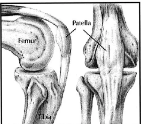
The patella is held in place by the quadriceps tendon superiorly and the patellar ligament (also known as patellar tendon) inferiorly, as it glides through the trochlea of the femur. The underside of the patella is divided into the medial, lateral, and odd facets, each of which is covered by articular cartilage that helps with shock absorption, smooth articulation, and load distribution (Figure 2.3).
N~ teii4a
Figure 2.3: Lateral and anterior view of patella and patella tendon.
The patella serves two important biomechanical functions in the knee. First, it increases the efficiency of the quadriceps muscle by increasing its lever arm. This provides a mechanical advantage by lengthening the extension moment arm throughout the entire range of knee joint motion, but in doing so, it is subjected to considerable retropatellar compression force. Second, it allows a wider distribution of compressive stress on the femur by increasing the contact area between the patella tendon and the femur [85].
Cartilage on the undersurface of the patella is the thickest of any found in the body. This thick joint cartilage acts as a cushion, absorbing shock in the greatest
2.1.4 The Menisci
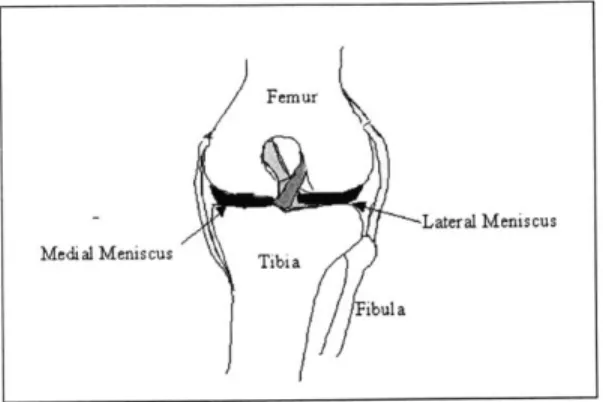
The menisci (Figure 2.4) are two fibrocartilagenous, semilunar structures with a wedge-shaped cross-section that lie between the opposing articulating surfaces (femur and tibia).
Femur
Lateral Meniscus
Medial Meniscus Tibia
Fibul a
Figure 2.4: Anterior view of left knee outlining the medial and lateral menisci.
The menisci's functions are [23]:
I. To serve as shock absorption to protect the articular surfaces of the bones,
II. To eliminate most of the direct tibial-femoral contact while increasing the surface
contact of the joint, thus reducing contact stress, III. To increase the elasticity of the joint,
IV. To assist in lubrication, and
V. To provide stability and increased range of flexion.
When a load is transmitted between the femur and the tibia, the vertical component tries to squeeze the meniscus out from between the articular surfaces. Hoop tension stiffness and stress act against that squeeze, to pull the meniscal wedge in between the opposing joint surfaces to maintain close contact and evenly distributed pressure in the wedge (Figure 2.5). This tends to float the femoral condyles above the tibial condyles. During this process, the high compliance in the flexure and shear allows the meniscus to deform
and adapt readily even to rapidly changing alignments of the articular incongruities. That unit loading over the whole meniscal surface in contact with cartilage tends to remain uniform. In the case that the menisci were to be removed, this load distribution effect will be altered, causing pain, bone wear and an increase in pressure on other joints, such as the hip, due to uneven load distribution on the knee joint. [4]. These effects may eventually result in joint degeneration.
A. B.
Femur
Femur AAA
Tibia Tibia
Figure 2.5: The effect of menisci on contact stresses: A. With menisci, B. Without the menisci.
2.2
Current Status of Knee Joint Biomechanics
Understanding the mechanism behind the load transmission in the knee joint in response to external loads plays an important role in the clinical world. It is not surprising that knee joint behavior has been studied extensively, both experimentally and computational, in the last two decades [24-29]. This brief review outlines the current status of knee biomechanics research.
2.2.1 Biomechanics of the Human Knee Joint
The human knee joint has been extensively studied. In many cases, knee joint motion was measured by rotary transducers [30], linearly variable differential transducers (LVDT), or rotational-variable differential transducers (RVDT) [31-33]. The motion of the tibia relative to the femur has also been measured using stainless steel pins that were
embedded into the bone to minimize skin motion [34-39]. Lewis et al. [34] developed an experimental system to quantify in vitro knee joint biomechanics. The system included an Instrumental Spatial Linkage (ISL) system for measuring 3D joint motion, buckle transducers for measuring ligament forces, and a pneumatic load apparatus for the application of external load. The ISL was composed of six revolute joints connecting two end links and five intermediate links. The motion of these joints was measured by potentiometers. Both femur and tibia were clamped onto the load apparatus but only the tibia was allowed to move (i.e. the femur was rigidly fixed).
Knee motion measured via geometrical properties is another way to study knee kinematics. Kurasawa et al [40] measured 3D knee motion by using the center of the posterior femoral condyles as a reference point. They analyzed sections of the distal femur by a computer and compared that to direct measurements to show that the femoral condyles can be approximated as spherical surfaces. They determined that from fully extended knee to 120 degrees of flexion the medial femoral condyle moved less than the lateral femoral condyle. Further, they observed an axial rotation of 20 degrees.
Light emitting diodes (LED) have been successfully applied in gait studies [35, 41]. Direct measurement of skeletal motion requires an invasive procedure to place pins on the bone. In many cases, external markers are used for similar analysis. Reinschmidt et al. [35] investigated the effect of skin movement on the analysis of knee joint motion. Skin markers were attached to three subjects. To compare the measurements obtained using the skin markers, bone pins were inserted as well. 3D kinematics of running trials were recorded using high-speed cine cameras (200HZ) and compared. They found that
the average errors relative to the range of motion during running were 21% for flexion/extension, 63% for internal/external rotation, and 70% for abduction/adduction.
A number of authors have studied passive knee joint motion, laxity, and stability.
Tools for control motions and external load application included instrumented handlebar [42, 43], instrumented fixtures in MTS* or Instron* testing machines [44-47]. Other investigators have used triaxial goniometer [43,48], photographic instruments [49], and roentgen-sterephotogrammetry (SPG) [24,50-56] to measure knee joint motion. Huiskes et al. [57] used analytical, closed-range sterophotogrammetry to determine the 3D geometry of the articular joint surfaces in-vitro. They projected a visible grid onto the articular surfaces. Glass rods with tantalum markers, firmly fixed to the bone, were used to inter-relate the articular surface geometry with the roentgenstereo-photogrammetry motion data. Blankevoort et al. [52] measured the in-vitro passive range of motion characteristics of the human knee joint under external loads using a 6 DOF motion rig. An accurate roentgen SPG system was applied for the measurement for geometric information. Human knees were used such that the tibia was free to move in 5 DOF relative to the fixed femur. Loading of the knee was done by applying weights to the part of the apparatus that was associated with the respective motion. Tantalum markers were placed on both bones to monitor the relative motion.
Many 6 Degree-of-Freedom (DOF) testing systems have been used for the measurement of knee joint kinematics under both in-vivo and in-vitro conditions [32, 33, 39, 52, 58-61]. Rudy et al [61-64] developed a robotics-based joint testing system that
offers the ability to control both the paths of motion as well as the acting forces. The system is composed of a 6 DOF robotic articulated manipulator and a universal
force-moment sensor (UFS). The testing of the knee specimen is done with the femur rigidly fixed to the robot base while the tibia is rigidly mounted to the robotic arm through the UFS. The system provides not only the measurement of structural properties, but also the
ability to store and repeat the 3D motion paths under different loading conditions. In response to external loads, the robot can learn the complex motion of the knee specimen. The system can then reproduce these motions in subsequent tests.
2.2.2 Biomechanics of Total Joint Replacement
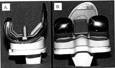
Knee replacements, commonly used today, differ from each other in material, fixation design, and more fundamentally, in their articular surface design [40, 65]. This wide range of available designs reflects different interpretations of the complex geometry of the natural joint surfaces. Desirable characteristics in knee prosthesis include durability, natural feeling, and interchangeability between sizes so that the femoral and tibial components can be fitted independently to their respective bones [6]. Three major TKA designs exist on the market:
I. PCL retention (PCR), where the PCL is saved (Figure 2.6),
II. PCL sacrificing (PCSac), where the PCL is resected but no substitution is added, and
III. PCL substitution (PCSub), where the PCL is resected but the implant design compensates for the absence of PCL (Figure 2.7).
Figure 2.6: Posterior cruciate retaining TKA (right knee). A. Lateral view, B. Posterior view.
Figure 2.7: Posterior cruciate substitution TKA (right knee). A. Medial view, B. Posterior view.
The role of PCL on knee joint function after TKA has been one of the most controversial issues in total knee replacement area. It has been argued that PCL retention in TKA can enhance joint stability, improve passive range of motion by allowing femoral roll back, increase the efficacy of the knee musculature, and reduce stresses at the cement-bone-implant interfaces [8, 66, 67]. Singerman [11] measured the surface strain of the PCL as a function of knee flexion angle and found that decreased posterior tibial slope increases strain in the PCL following TKA. Using a combined buckle transducer
technique and computer modeling, Lew and Lewis [9] reported that PCL forces with a low conformity design were similar to those in the normal knee, but were substantially higher between 600 to 900 of flexion for a high-conformity design. Follow-up studies of patients post TKA showed that partial release of the PCL is beneficial for patients with tight PCL at the time of knee arthroplasty. This partial release procedure improved maximum flexion angle and maintained anterior-posterior stability [12, 68]. It was suggested by Freeman and Railton [69] that PCL may contribute to posterior stability in a flexed knee if its tension can be accurately restored. However, normal tension of the PCL is often difficult to obtain [6]. Researchers [70, 71] analyzed the joint kinematics of TKA with PCL retention and found that physiological rollback of the femur was not demonstrated for patients after a PCL retaining TKA. Dennis et al [13] observed abnormal femoral translation during deep knee bends of patients after TKA. Further, they demonstrated that the TKA with PCL retention has a similar passive range-of-motion (ROM) to TKA with PCL substitution, but a decreased ROM during squatting compared with the PCL substituting TKA. Long term patient follow-up studies revealed no differences between knee scores or long term survival rates in patients after TKA with PCL retention and TKA with PCL substitution [65, 72, 73]. Laskin [74] reported that TKA with PCL retention in rheumatoid arthritis increased posterior instability and recurvatum deformity, resulting in an increased revision rate. Recently, there are reports showing that the preservation of the PCL in TKA may not improve knee joint proprioception and subsequently may not improve TKA functional performance [41, 75].
Chapter 3
ROBOTIC TESTING SYSTEM FOR
TKA BIOMECHANICS
The desired purpose of a TKA is to restore normal joint function, which includes both kinematics and kinetic restorations. Hence, the TKA should restore the knee joint motion in 6-DOF as well as, joint pressure, ligaments tension, and patella contact mechanics. It is a challenge to quantify the biomechanical responses of the intact knee and the knee after TKA using the same knee specimen.
It is therefore the objective of this project to develop a non-contact, 6-DOF experimental system for measuring knee kinematics, tibio-femoral joint forces and ligaments forces under simulated external loading conditions. The test system is composed of a 6 degree-of-freedom (DOF) robotic manipulator (Kawasaki UZ150*, Kawasaki Heavy Industry, Japan) and a 6 DOF load cell (JR3 DSP-based force sensor receiver, JR3 Inc., Woodland, CA). A control algorithm that uses global convergence method [77] that considers the coupling effects of the different DOF of the knee was developed in this project. This algorithm links the robot and the load cell so that both displacement and force controls are available.
3.1
Displacement Control Device: Robot Manipulator
3.1.1 General Description'
The robotic system is composed of two main components: the robotic arm manipulator
and the C controller (Figure 3.1). The Kawasaki UZ150* manipulator consists of rigid links which are connected with six joints that allow relative motion of the neighboring links. The manipulator is equipped with six stepper motors that can directly execute a desired trajectory (position control capability). A movement of the manipulator to follow a desired route is achieved by a position control system that uses feedback from joint sensors to keep the manipulator on course. The C controller offers a large,
multi-functional color liquid crystal display (LCD) that combines the functions of a conventional teach pendant with several specialized displays on an 8-inch touch panel. Easy block-step programming and high-end AS language programming are both available. This AS language allows a wide range of robot control commands, numerical calculations, conditional jump step divergence, interrupt I/O and program creation on PC. The controller's multitasking capability allows parallel programs to run simultaneously while the robot is moving, and simple sequences do not require the use of a sequencer.
b. &
Figure 3.1: The components of the robotic system: a. Kawasaki UZ1 50 manipulator; b. C-Controller.
Table 3.1 summarizes some of important specification of the UZI50 model.
Axes 6z
Table 3.1: UZ 150 selected specification.
Payload Repeatability
150 Kg
±0.3
mmThe repeatability value reported here is for full load, extended arm, and high-speed (1000mm/sec) operation. For a more confined space and slower speed as used in the knee joint experiment, this value is reduced dramatically.
3.1.2 Communication with Personal Computer (PC)
The robotic system can be controlled either by the C-controller (AS language) or by a host computer via a serial port. In this project, a personal computer (Dell Dimension 3DX) was used in the control procedures. A serial (RS232) interface was constructed between the C controller and the PC to allow information on the robot location to be transferred between the two systems. Through a specified protocol, ASCII characters were sent and received on the serial interface line. A basic handshaking protocol was
used in this project (Figure 3.2).
'05' '02' '03' '04' E E E N T TEXT T 0 Sender Q x T '06' A A C C Receiver K K
Figure 3.2: Communication protocol.
(ENQ, query; ACK, acknowledgment; STX, start text; ETX, end of text; EOT, end of transmission) Both the controller and the PC had to be programmed to communicate with each other following the above protocol. A Visual Basic (VB, Microsofte Visual Basic 6.0) code was developed for the PC and AS code was written for the controller. In this project, the current position of the robot is crucial at all times. This is done by the robot sending its location using the AS command SEND 2: $out, err and the PC reading the ASCII dada using VB code C = MSComml.Input. The robot command for receiving information from the PC is RECEIVE 2: $inp, err, while the VB code for sending information to the robot is MSComml.Output = a. All communication programs developed in this project are listed in Appendix B.
3.2
Force Control Device: JR3 Universal Force/Moment
Sensor
3.2.1 General Description
2The addition of the 6-DOF JR3* Digital-Signal-Processing (DSP, analog Devices ADSP-2105) load cell onto the end effector of the robotic manipulator provides the system with
the ability to control forces applied to the knee joint (force control capability). The JR3 system provides the user with decoupled and digitally filtered force and moment data at 8 kHz per channel. The system uses a dual ported Random-Access-Memory (RAM) that the user and the JR3 DSP can both read and write to. Forces and moments are written by the JR3 DSP into this RAM. The user can then read the data from the RAM. The dual-ported address space consists of 16K 2-byte words. The first 8K of this space are used as RAM while the second half consists of status registers and other features. The DSP performs several functions such as offset removal, saturation removal, digital low-pass filtering, peak detection, force and moment vector calculations, threshold monitoring, rate calculations, and coordinate system translation and rotation. The raw data from the sensor is decoupled and passed through a series of low-pass-filters (LPF). There are eight filters; the first filter has a cutoff frequency of 500Hz and each succeeding filter has a cutoff frequency of 1/4 of the preceding filter (i.e. 500Hz, 125 Hz, 31.5Hz, 7.81Hz, etc). The delay through the filters can be approximated as the inverse of the cutoff frequency. For example, the delay through the third filter (31.5 Hz) would be 1/31.5 31.7msec.
The data structure declarations of the JR3 system are formatted in 'C' style code. The following code outlines several important definitions used in the AS code. The code defines a signed 16-bit integer value, uses an array to include force and moment data, as well as read and write from a given address:
intfx /* signed 16-bit value for storing the x component of the force */
unsinged data array[6] /* unsigned 16-bit array to include 3 forces and 3 moments */
readData (0xJ005) /* read the version number of the DSP software */
writeData (OxOOe7, 0x0800) /* write the value 0x800 to the OxOOe7 location */
3.2.2
JR3 DSP Based Force Sensor Receiver Card
The receiver card plugs into a 16-bit connector on the ISA bus. The receiver operates typically on 5V and 650mA, obtained directly from the ISA card.
The DSP receiver board uses two 16-bit wide registers. The address register is at I/O addresses zero and one relative to the base address. In this project the base address was set to 0x314. It can be concluded that the first 16-bit port at 0x314 represents the address port while the second 16-bit port, i.e. 0x316, represents the data port. The card address can be changed to fit other addresses by selecting the right switch combination. Figure 3.3 demonstrates the switch position for 0x314 address.
1 1 0 0 0 1 0 1 0x314
Figure 3.3: Address selection for the ISA bus receiver.
3.2.3 System Set-up: Force and Moment Measurements
As mentioned before, unfiltered data, as well as filtered data, can be collected from the sensor. Although all filters meet our criteria, in this project, data subsequent to the third filter (low pass filter of 31.5 Hz) has been used (data address &HA8). The data collection program is based on a previous program written by Commotion Technology (Commotion Technology, Inc. World Trade Center, Suite 250-L, San Francisco, CA 94111). The general loop for reading forces and moments is listed below:
JR3read(boardNum, CFORCE + i, force)
bourdNum is the board number (0x314),
C_FORCE is the address for the force / moment data (Oxa8),
i is the index for consecutive loop operations for three forces and three moments, and force is the returned value from the sensor.
Different JR3 sensors make use of different measurement units. The JR3 2000N load cell, used in this project, makes use of SI units (N, Nm*10 for forces and moments, respectively). Note the moment units as being multiplied by ten. This is done for a more accurate reading of the lower end of the moment scale.
The capacity of JR3 load cell used in this project is shown in Table 3.2 below. Table 3.2: JR3 sensor specific information.
Model Dimension Loads3
160M50S 160mm diameter 2000N
50mm thickness 250Nm
3.2.4 Zeroing the Load Cell
As in every engineering system, a reference point (level) must be determined. Therefore, all values of the load cell had to be zeroed at the beginning of the experiment such that all other measured values are with respect to this zero. The following code was written in VB to zero the force and moment values of the load cell. Note that this procedure is qn1Y done once and at the beginning of each experiment.
Private Function zeroJR3( As Boolean
Dim i As Integer, value As Integer, error As Long, offset As Integer
'6 components: 3 forces 0,1,2 and 3 moments 3,4,5
For i = 0 To 5
'Read current offset
error = JR3read(0x314, 0x88 + i, offset)
3 The sensor load rating is the full scale rating for the X or Y axis. The Z axis full scale rating is twice the sensor rating.
If error <> 0 Then
Err.Raise vbObjectError + error
End I
'Read current force
error = JR3read(0x314, Oxa8+ i, value)
' Update current offset
error = JR3write(0x314, Ox88 + i, offset + value) Next I
ZeroJR 3=True End Function
This general procedure involves reading:
I. The offset for each of the variables (three force components and 3 moment
components) from the DSP 0x88 location
II. The force and moment components (six total) from the DSP Oxa8 location. This location displays the data from filter #3.
Once these two quantities are read, a correction is made to the corresponding offset addresses.
3.2.5
Load Cell Calibration
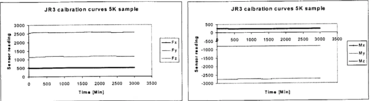
The stability of the load cell over time is critical in this project since a typical testing session lasts about 15 hours. Further, the accuracy of the load cell had to be determined to ensure its suitability for the project (see section 4.2). Therefore, calibration of the load cell was performed in two ways. First, the response of the load cell readings over time was recorded to ensure that drifting, due to internal electronic devices, is minimal. Second, the response of the load cell to external loads was obtained by using standard weights. Figures 3.4, 3.5, and 3.6 display the results for the calibration process.
JR3 calbration curves 5K sample 3000 --m 2500 -2000 1500 .-- Fy 1000 500 0 500 1000 1500 2000 2500 3000 3500 Time [Min]
JR3 calbration curves 5K sample
500 0 -500 -" 500 1000 1500 2000 2500 3000 35 00 * -1000 M -1500 -M -2000 -2500 -3000 Time [Min]
Figure 3.4: Forces and moments drifting behavior of the JR34 during 50 hours of operation.
S350 0.97x -0.51 R2 I 300 250 e 200 i F Aveg 150 . 100 50 5h [ W e ig hts [NJ 3 0 0 - - ~ ~ ~ ~ ~ ~ ~ ~ ~ ~ ~ ~ ~ ~ ~ ~ ~ ~ y =0.93x + 0.16 250 200 150 Avrrge 100 0 50 0 0 100 200 300 400 W e ights [N]
Figure 3.5: Force calibration in the x and y directions.
50 - 0 -5 " ion 0 I50 4 0 -100 w -150 *Fz -Average -200 S-250 o y = -0.99x -0.32 -J 300R 2 1 -350 Weighs [N] 30 y = 1.04x -0.13 25 R = 0.9999 z 20 E 15 10 0 5 10 15 20 Calculated Mz [Nm]
Figure 3.6: Force (z direction) and moment (around z) calibration.
Similar results were obtained for the moment around X and Y axes. The above results show that the load cell meets the calibration standards set for this project.
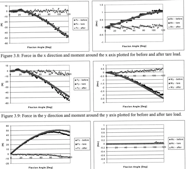
3.2.6 Load Cell Tare Load: The Effect of Gravity
Recall that the load cell and fixture rotate with the robot arm. One of the most dramatic effects of this rotation can be seen in the force and moment readings of the JR3 LC as the effect of gravity comes into play. To account for these gravitational effects, the VB program for reading the LC was modified. First, the load cell and the attached fixture weight were measured. Further, the center of rotation for the load cell - fixture assembly was determined (see Figure 3.7). These calculations were incorporated into the load cell reading to cancel out the gravitational effect. Figures 3.8, 3.9, and 3.10 display selected plots of load cell reading before and after the tare load effect.
Center of load cell, where measurements
+z' are recorded
Fixture
0.023 m
Center of load cell fixture assembly
0.0414 m
Figure 3.7: Load cell - fixture assembly.
Equations 3.1 and 3.2 describe the general procedure to compensate for the effects (gravitation, and moments) of the fixture assembly on the load cell reading:
1 = A ead by the load cell + +oa mVnitial anitial Globa CS CSR) (3.2)
Where:
F is a vector (3x1) representing the forces (Fx, Fy, F,) at any given flexion angle
accounting for the gravitational effect of load cell and fixture,
read by the load cell is a vector representing the forces (x, y, z) read by the load cell (not
including gravitational effect),
WLadcellCS is the weight of the load cell - fixture assembly in load cell coordinate
system,
Roa, is a 3x3 rotation matrix (zyz sequence) to transform a vector from the global
system to the local system (load cell),
WGlobal CS is the weight of the load cell - fixture assembly in global coordinate system,
M is a vector (3x1) representing the moments (mx, my, mz) at any given flexion
angle accounting for the gravitational effect,
Mread by the load cell is a vector representing the moments (mx, my, m,) read by the load
cell (not including gravitational effect),
min-,,i0 , is the initial moment read by the load cell due to the fixture assembly, and
F is the three dimensional position vector between the load cell center of rotation and
the fixture center of rotation written in load cell coordinate system
r = [0.023,0,0.0414] (Figure 3.7).
A VB procedure was written to account for the load cell - fixture assembly gravitational effect for every flexion angle (see Appendix D).
10 . . -10 20 0 80 100 1 0 -20 - Fx -before -30 -40 -50 -60
-Flexion Angle [Deg]
1.5 -0.5 -Mx -before E *Mx - tare 0 4M xN- after 20 40 60 80 100 1 0 -0.5 -1 -F---A--l
[-Flexion Angle (Dug]
Figure 3.8: Force in the x direction and moment around the x axis plotted for before and after tare load.
10 0 4 i -i 20 60 80 tWkW 0 -0 --20 -* Fy -before z eFy -tare -30 Fy -after -40 -50 -60 - - - ~--- ----
-Flexion Angle [Dog]
Figure 3.9: Force in the y direction and moment around
1 0.5 0 -0.5 -1 *My -before - - My-tare .2 -2 - My -after -2.5 -3 -3.5 -4
Flexion Angle [Deg)
the y axis plotted for before and after tare load.
60 50 40 30 -Fz -before 220 *Fz -tare 10 20 a Fz -after -10 -20Fx-- n Angie ig] --Flexion Angle [Dog]
1 0.8 0.6 0.4 0.2 +Mz -before E 2 o~ e Mz -tare -0.2 1 2 0B 1h.' Mz-after -0.4 -0.6 -0.8 -1
Flexion Angle [Dog]
Figure 3.10: Force in the z direction and moment around the z axis plotted for before and after tare load.
3.3
Digitization System
Coordinate systems of the knee and of the load cell are required for the calculation of the relative motion of the tibia with respect to the femur. An Immersion MiscroScribe 3DX (Immersion Corporation, CA) digitizer is used to establish these coordinate systems.
The MicroScribe-3DX is a tool for performing 3-dimentional digitizing. Its communication with a PC is done through a standard RS-232 serial port. Figure 3.11
'Wrist Roir' Elbow Joint LowerArm Joint
Segment
"Wrst Pitch*
Stylus Stylus
Tip Upper Aim
Stylus Segment Holder Shoulder Joint /--'Tombstone" Counterweight 1 z Base L Yont NIkI. -Base
Figure 3.11: MicroScribe parts and features.
The system includes the arm unit, which houses the internal electronics, a serial cable, and an external module. The MicroScribe is connected to COM2 serial port of the PC. A double foot pedal is attached to the rear panel of the digitizing arm for hand-free
data selection. The system makes use of five optical sensors to record the relative angles of the device such that the tip location (x, y, and z) is reported. In this project, the stand-alone program called InScribe (developed by Immersion Corporation) was used for data accumulation. This application runs in the background of Windows, entering coordinate values (x, y, and z) directly into Microsoft Excel (V.97). Table 3.3 below lists some of the important features of the MicroScribe-3DX.
Table 3.3: MiscroScribe-3DX selected specification.
Workspace Position Sampling Rate
Accuracy
Chapter 4
FORCE AND DISPLACEMENT
CONTROLS OF THE TEST SYSTEM
4.1
General Description
In the robotic system introduced in Chapter 3, the load cell is rigidly fixed to the end of the robot arm and is free to move with arm motion. The robotic test system controls the position of the knee in space by learning (force control) and replaying (displacement control) predetermined positions of the knee. In this chapter, a detailed description for the development of force and displacement control algorithms for human knee test is presented.
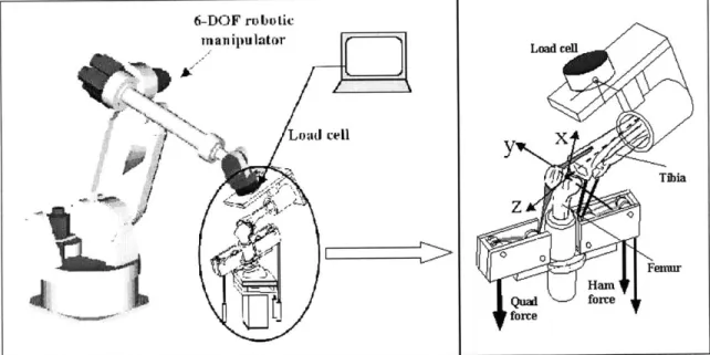
4.1.1 Experimental Set-up
In this project, the tibia is mounted on the robotic manipulator through the load cell while the femur is rigidly fixed onto a pedestal. This allows the robot to move the tibia while the femur remains fixed. In this project the knee is placed in an inverted orientation compared to its physiological orientation. Two reasons for this set-up: clinically,
surgeons manipulate the tibia to evaluate TKA stability. Further, the application of muscle loads is done easily when the knee is inverted.
The knee specimen is aligned so that the load cell can measure three force and three moment components along and about a cartesian coordinate system. The longitudinal axis of the tibia (x), the epicondylar (medial-lateral) axis of the femur (y), and the anterior-posterior axis of the knee (z) define the coordinate system (Figure 4.1). The origin of the system is chosen as the midpoint of the trans-epicondylar line.
6-DOF ro botic iiianipulator Load cell Poll, Load cell - - Fermr Ham Quad fre force
Figure 4.1: Set-up of the robotic testing system
The femoral coordinate system and the tibial coordinate system coincide with each other at full extension of the knee (also called initial position) under no load condition [76]. Thus, only one coordinate system is needed to be defined initially (Figure 4.2a). As the knee responds to external load, the tibial coordinate system moves with the tibia. At that point, the coordinate system of the femur no longer coincides with the coordinate system of the tibia. Therefore, the translation vector and the rotation matrix of the tibia with respect to the femur must be evaluated to determine the knee kinematics (Figure 4.2b).
a. femur x y Z t tibia b. femur x femur y Z X tibia tibia
Figure 4.2: Tibia and femur coordinate system (CS) configuration: a. femur and tibia CS coincide, b. rotated tibia.
There are many ways to construct the initial knee coordinate system (ruler, optical markers, etc.). In this project, the MicroScribe* 3DX, described in section 3.3, was utilized for the digitization of the anatomical points of the knee. These points were then
used to reconstruct the knee coordinate system.
4.1.2 Coordinate System Development
The knee coordinate system was constructed by digitizing (MicroScribe 3DX*) four anatomic points on the knee (Figure 4.3). Two points parallel to posterior cortex in the longitudinal direction of the tibia (C, D), and midpoints of the insertions of the medial and lateral collateral ligaments (A, B) were specified on the specimen. In addition, the
load cell coordinate system was established by digitizing three points (U1, U2, U3) on the
U1 U2 U, D Cylinder F C Tibia B A ) (Femur IF +
Figure 4.3: Coordinate system determination for load cell and knee.
The knee and load cell axes, as well as their center of rotation were calculated from these digitized points. Table 4.1 presents the major equations involved in these calculations.
Table 4.1: Coordinate system calculations for load cell and knee.
Center x-axis y-axis z-axis
Load Cell - + U3 6U - 2 u-2 1-3 XY Knee Femur: i-O A±BXX Of= 2 Tibia:
0,
= Of+ (D- C)A VB subroutine was written to construct the coordinate system from the digitized points
and to calculate the relative rotation (RLK) and translation vector (rkl) between the knee and the load cell (see Appendix E).
4.1.3 Knee-Load Cell-Digitizer Relationship
The relative orientation and translation of the tibia with respect to the femur is of interest. Since the tibia is rigidly fixed to the load cell, the relative orientation and translation of the load cell with respect to the femur are to be measured. Figure 4.4 presents a diagram
relating the digitizer, load cell, and knee. In this section, only the kinematics data is presented. Table 4.2 summarizes the variables involved in this process.
Load Cell
(1)
ld; il
A p
.(k)
A '
Digitizer (d)
Figure 4.4: Schematic diagram of digitizer, load cell, and knee kinematics.
Table 4.2: Variables description.
Symbol Description
rdk Translation vector from digitizer to knee
rdl Translation vector from digitizer to LC
rlk Translation vector from LC to knee
Rkd Rotation matrix of knee relative to digitizer
Rd Rotation matrix of LC relative to digitizer
Rkl Rotation matrix of knee relative to LC
The following VB code was written to construct the translation vector Fdk and the rotation
matrix Rkd :
'read the points A, B, C, D, and Efrom a tab delineated file
Input #11, Ax, Ay, Az, Bx, By, Bz, Cx, Cy, Cz, Dx, Dy, Dz, Ex, Ey, Ez, Fx, Fy, Fz 'calculating center of rotation for the femur