Processes controlling the distribution of dissolved silicon isotopes (δ30Si) in the Atlantic and the Southern Ocean

HAL Id: tel-01630072

https://tel.archives-ouvertes.fr/tel-01630072

HAL is a multi-disciplinary open access archive for the deposit and dissemination of sci-entific research documents, whether they are pub-lished or not. The documents may come from teaching and research institutions in France or abroad, or from public or private research centers.

L’archive ouverte pluridisciplinaire HAL, est destinée au dépôt et à la diffusion de documents scientifiques de niveau recherche, publiés ou non, émanant des établissements d’enseignement et de recherche français ou étrangers, des laboratoires publics ou privés.

Processes controlling the distribution of dissolved silicon

isotopes (δ30Si) in the Atlantic and the Southern Ocean

Nathalie Coffineau

To cite this version:

Nathalie Coffineau. Processes controlling the distribution of dissolved silicon isotopes (δ30Si) in the Atlantic and the Southern Ocean. Other. Université de Bretagne occidentale - Brest, 2013. English. �NNT : 2013BRES0067�. �tel-01630072�

4

To my amazing family…

8

concentration en DSi et δ30Si au moment de l'échantillonnage. Les masses d'eau de fond ont été caractérisées par un faible δ30Si de 1,1 ‰, légèrement inférieur au δ30Si de 1,2 ‰ trouvé dans les eaux de fond du courant circumpolaire antarctique (ACC). L'influence de l’eau de fond Nord Atlantique (NADW) par l’eau de fond circumpolaire (UCDW) a été observée à la fois dans le passage de Drake et au niveau du méridien de Greenwich pour le _δ30_{Si. Nos données confirment la présence} du gradient de δ30Si dans les masses d'eau profondes ; gradient déjà proposé et décrit par de fort δ30

SiDSi (≥ 1,7 ‰) pour l’eau de fond Nord Atlantique (NADW) dans le nord de l'océan Atlantique Nord et par de faible δ30SiDSi (1,2 ‰) pour l’eau de fond antarctique (AABW) enregistré dans l'océan Austral.

13

mbsl) for the A) δ30

Si evolution versus depth, error bars on δ30Si represent standard error on 2–3 separate measurements, the arrow indicates the Last Glacial Maximum (LGM) and B) BSi against depth. The percentage opal (P. N. Froelich, unpublished data) was determined through extraction into a sodium carbonate solution 32. Modified from De La Rocha et al. (1998). ... 19

Chapter 2: Method and analytical techniques

Figure 2.1 Protocol for DSi precipitation via TEA-moly and extraction ... 25

Figure 2.2 A) Neptune (Thermo Fisher Scientific), B) Main parts of the Neptune, the Inductively Coupled Plasma module (ICP Module), the Electrostatic Analyzer module (ESA Module) and the Multi-collector module (wwz.ifremer.fr/neptune). ... 27 Figure 2.3 Samples measurement of the ratio δ29Si vs. δ30Si for A) ANTXXIII/9 campaign, B) ANTXXIV/3 campaign and C) MSM10/1 campaign, along the fractionation line δ30_{Si = 1.93 · δ}29_{Si. Each session on} the MC-ICPMS is represented by a different colour, standard deviation (1 σ). ... 33

Chapter 4: The silicon isotopic composition (δ30Si) of water masses in Atlantic Ocean

Figure 4.1 The great conveyor belt. Representation of warm surface currents (red), cold deep currents (blue) and bottom currents (purple). Circles: sites of deep water formation, white zones: salinity < 34, dark blue: salinity > 36 psu, (Kuhlbrodt et al., 2007). ... 61 Figure 4.2 Map of the Subtropical and Tropical North Atlantic Ocean circulation. The dashed and dotted line represent the Cape Verde Frontal Zone (CVFZ), the North Equatorial Current (NEC), the northern band of the South Equatorial Current (nSEC), the North Equatorial Countercurrent (NECC) and around the Guinea Dome is found the northern NECC (nNECC) as labelled on the plot (Stramma et al., 2005). ... 63 Figure 4.3 A schematic view of the map of meridional overturning circulation in the Southern Ocean (Speer et al., 2000; Dong, 2012). SAMW is the surface water, AAIW is the Antarctic Intermediate Water, UCDW is Upper circumpolar Deep Water, NADW is North Atlantic Deep Water, LCDW is Lower Circumpolar Deep Water and AABW is Antarctic Bottom Water. ... 65 Figure 4.4 Mean solution composition showing concentration (greater than 50%) of all source water types along Section 1 of ANT-XXIII/3 in the Drake Passage. Gray colour represents a mixing of SWTs without major contribution of any SWT (white contours represent neutral density values) (Sudre et al., 2011). ... 66 Figure 4.5 Section along the prime meridian in the Southern Ocean and in the Weddell Gyre showing potential temperature (θ(°C)) and the generalized locations and movements of various water masses. The region between 40°S and 55°S represents the Antarctic Circumpolar Current (ACC). The region from 55°S to 70°S represents the actual Weddell Gyre. AAIW: Antarctic Intermediate Water, NADW: North Atlantic Deep Water, CDW: Circumpolar Deep Water, AABW: Antarctic Bottom Water, SHALLOW: the shallowest 200m of the water column, WDW: Warm Deep Water, WSDW: Weddell Sea Deep Water and WSBW: Weddell Sea Bottom Water (van Heuven et al., 2011). ... 67

14

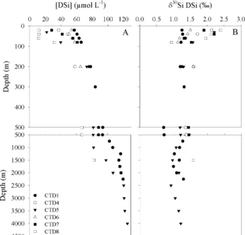
sampled in the Subtropical and Tropical Atlantic Ocean (MSM10/1 campaign) and red dots indicate stations sampled in the Southern Ocean (ANTXXIV/3 campaign). Stations from which samples were analysed are encircled and numbered (Schlitzer, R., Ocean Data View, http://odv.awi.de, 2013). ... 71 Figure 4.7 Temperature–salinity depth profiles of stations from ANTXXIV/3 campaign. A) Full depth profiles, B) zoom in on stations (146, 189 and 211) in the Weddell Gyre. Modified from Mackensen (2001). ... 73 Figure 4.8 Longitudinal transect through Weddell Gyre realized with data from ANTXXIV/3 campaign. Our stations 211 and 189 are indicated by vertical lines. Thin horizontal lines indicate temperature boundaries. Salinity colour maps were created with ODV (Schlitzer, Ocean Data View, http://odv.awi.de, 2013) using data from ANTXXIV/3 campaign. ASW: Antarctic Surface Water, MWDW: Modified Warm Deep Water, WDW: Warm Deep Water, WSDW: Weddell Sea Deep Water and WSBW: Weddell Sea Bottom Water. ... 74 Figure 4.9 Latitudinal transect of Drake Passage realized with data from ANTXXIV/3 campaign. Our stations 248 and 226 are indicated by vertical lines. Thin horizontal lines indicate salinity boundaries. Potential temperature colour maps were created with ODV (Schlitzer, Ocean Data View, http://odv.awi.de, 2013) using data from ANTXXIV/3 campaign. SASW: Subantarctic surface Water, SAMW: Subantarctic Mode Water, AAIW: Antarctic Intermediate Water, SPDSW: Southeast Pacific Deep Slope Water, UCDW: Upper Circumpolar Deep Water, LCDW: Lower Circumpolar Deep Water, SPDW: Southeast Pacific Deep Water, WSDW: Weddell Sea Deep Water. ... 75 Figure 4.10 Latitudinal transect on the 0° meridian realized with data from ANTXXIV/3 campaign. Our stations 106, 115 and 146 are indicated by vertical lines. Thin horizontal lines indicate temperature boundaries. Salinity colour maps were created with ODV (Schlitzer, Ocean Data View, http://odv.awi.de, 2013) using data from ANTXXIV/3 campaign. ... 76 Figure 4.11 Temperature – Salinity diagram for Atlantic Ocean water masses. Coloured lines indicate stations sampled during MSM10/1 campaign: station 1 (green), 2 (red), 3 (pink), 4 (brown), 21 (blue). SACW: South Atlantic Central Water, wNACW and eNACW: western and eastern North Atlantic Central Water, MW: Mediterranean Water, NADW: North Atlantic Deep Water, AABW: Antarctic Bottom Water, AAIW: Antarctic Intermediate Water, WASIW and EASIW: western and eastern Atlantic Modified from Emery (2003). ... 77 Figure 4.12 Latitudinal transect of the Subtropical and Tropical Atlantic Ocean realized with data from MSM10/1 campaign. Our stations 1, 2, 3, 4 and 21 are indicated by vertical lines. Thin horizontal lines indicate temperature boundaries. Salinity colour map was created with ODV (Schlitzer, Ocean Data View, http://odv.awi.de, 2013) using data from MSM10/1 campaign ... 77 Figure 4.13 Depth profiles of DSi concentration (A, C, E, G, I, K, M, O, Q, S, U, W) and δ30Si (B, D, F, H, J, L, N, P, R, T, V, X) for the Southern Ocean (ANTXXIV/3 campaign, A to N) and for the tropical and subtropical Atlantic Ocean (MSM 10/1, O to X). Stations 226 and 248 were located in the Drake Passage; 248 was part of the Antarctic Circumpolar Current (ACC); 211, 189 and 146 were located in the Weddell Gyre (WG); 146 was at the edge of the WG and the ACC on the 0° meridian; and 106 and 115 were part of the ACC along the 0° meridian. Station 115 (K, L) is on a shallower depth scale (0 – 1000 m) than other stations of the Southern Ocean. Stations 1, 2 and 3 were north of the Cape Verde Frontal Zone (CVFZ), and stations 4 and 21 were south of the front. The depth and DSi concentration scales for the subtropical and tropical Atlantic Ocean are smaller than the Southern Ocean. ... 79

15

the Antarctic Circumpolar Current (ACC) and in the Weddell Gyre. (Station 146 was not taken into account for the regression). ... 82 Figure 4.15 Deep water masses of the Weddell Gyre showing δ30SiDSi versus longitude. Station 211 represents the western part of the gyre, 189 the central part and 146 is on the 0° meridian in the Weddell Gyre. WDW: Warm Deep Water, WSDW; Weddell Sea Deep Water and WSBW: Weddell Sea Bottom Water. ... 83 Figure 4.16 Longitudinal transect through the Weddell Gyre realized with data from the ANTXXIV/3 campaign. Our stations 211 and 189 are indicated by vertical lines that represent in the same time the δ30

SiDSi of 1.2 ‰ characteristic of deep water masses value in the Southern Ocean. Grey lines with diamond markers represent δ30_Si

DSi profiles. Thin horizontal lines indicate [DSi] boundaries. DSi concentration colour map was created with ODV (Schlitzer, Ocean Data View, http://odv.awi.de, 2013) using data from ANTXXIV/3 campaign ... 86 Figure 4.17 Depth profiles until only down to 1000 m at station 146 for A) salinity, B) temperature (°C), C) DSi concentration (µM) and D) δ30

SiDSi (‰). ... 86 Figure 4.18 Latitudinal transect through the Drake Passage realized with data from the ANTXXIV/3 campaign. Our stations 248 and 226 are indicated by vertical lines that represent in the same time the δ30

SiDSi of 1.2 ‰ characteristic of deep water masses value in the Southern Ocean. Grey lines with diamond markers represent δ30

SiDSi profiles. Thin horizontal lines indicate [DSi] boundaries. DSi concentration colour map was created with ODV (Schlitzer, Ocean Data View, http://odv.awi.de, 2013) using data from ANTXXIV/3 campaign ... 87 Figure 4.19 Latitudinal transect through 0° meridian realized with data from the ANTXXIV/3 campaign. Our stations 106, 115 and 146 are indicated by vertical lines that represent in the same time the δ30

SiDSi of 1.2 ‰ characteristic of deep water masses value in the Southern Ocean. Grey lines with diamond markers represent δ30

SiDSi profiles. Thin horizontal lines indicate [DSi] boundaries. DSi concentration colour map was created with ODV (Schlitzer, Ocean Data View, http://odv.awi.de, 2013) using data from ANTXXIV/3 campaign. ... 88 Figure 4.20 Representation of the A) DSi concentration versus latitude and B) δ30Si versus latitude for data from intermediate and deep water masses of the Atlantic Ocean from the literature for which data for DSi concentration and δ30Si were available (de Souza et al., 2012b; Fripiat et al., 2012), including data from this study. A) Regression line: R² = 0.80, p < 0.0001 and n = 140, and B) Regression line: R² = 0.34, p < 0.0001 and n = 140. Black diamond: deep water masses, grey diamonds: intermediate water masses, both were used in the calculation of the regression lines .... 93

1

Introduction - General context

─ Chapter 1 ─

2

Chapter 1 – Introduction

I Silica cycle

I.1 General

Even if silicon (Si) is the 2nd most abundant element of the Earth's crust (Epstein, 1999) it is mainly inaccessible for organisms as it is found in association with oxygen as quartz and silicate minerals (Laruelle et al., 2009). Its participation in terrestrial and marine biogeochemical cycles ultimately results from the weathering of silicate minerals and rocks. The weathering process releases essential nutrients, making them available to aquatic and terrestrial organisms (Ziegler et al., 2005). The release of Si during weathering to yield dissolved silicon (DSi) in soil water, groundwater, river water, and seawater leads in part to the incorporation of Si into biogenic silica (BSi), e.g., phytoliths in land plants (Ziegler et al., 2005; Cardinal et al., 2010; Opfergelt and Delmelle, 2012). The DSi released during weathering may be transported, via rivers and groundwater, to the ocean (Opfergelt and Delmelle, 2012). Some of the Si released through silicate weathering becomes incorporated into clay minerals, but silicon is still such a major element of silicate rocks that dissolved silicon is the dominant nutrient in river waters, and rivers supply roughly 80% of the silicic acid added to the ocean each year (Tréguer et al., 1995; Ziegler et al., 2005; Tréguer and De La Rocha, 2013). Silicon cycling is strongly linked to climate inasmuch that the chemical transformation of silicate rocks into solutes through weathering requires atmospheric CO2 (Berner et al., 1983; Georg et al., 2007).

The dissolution of silicate minerals converts atmospheric CO2 into alkalinity (carbonate and bicarbonate ions) as with the following idealized example:

. (1.1)

This addition of alkalinity to the ocean, in turn, governs the oceanic capacity to hold dissolved CO2. At typical seawater pH (7.5 – 8.4), Si(OH)4, the undissociated form of silicic acid, is the most abundant, accounting for 97% of the dissolved silicon, with about 3% of it present as its dissociated anion, SiO(OH)

-3. In the long term, the solutes added to the ocean from silicate weathering are removed, for example, via the production of calcium carbonate and biogenic silica (BSi) by plankton such as diatoms, requiring silicon and the removal of these materials to the sediments (Dessert et al., 2003). Eventually these CaCO3 and SiO2 sediments will be subducted back into the mantle along with

4 4 -3 + 2 3 2

2atm

3H

O

+

CaSiO

Ca

2HCO

+

H

SiO

3

later through volcanism.

I.2 The silicon input pathways to the ocean

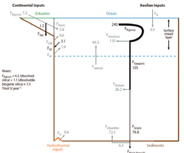
According to Tréguer and De La Rocha (2013), there are four pathways for the transfer of silicon to ocean estimated to bring to the ocean 9.4 ± 4.7 Tmol-Si yr-1 (Fig. 1.1).

Figure 1.1 The steady state biogeochemical cycle of silica (Tréguer and De La Rocha, 2013) (adapted from Tréguer et al. (1995)).The dotted line represents the limit between the estuaries and the ocean. Gray arrows represent fluxes of DSi and black arrows represent fluxes of BSi; all fluxes are in teramoles of silicon per year. Abbreviations: FR(gross): gross river inputs, FR(net): net river inputs, FRW: BSi deposits and reverse weathering in

estuaries, FGW: groundwater flux, FA: aeolian inputs, FH: hydrothermal inputs, FW: seafloor weathering inputs,

FP(gross): BSi gross production, FD(surface): flux of DSi recycled in the surface reservoir, FE(export): flux of BSi

exported toward the deep reservoir, FD(deep): flux of DSi recycled in deep waters, FD(benthic): flux of DSi recycled

at the sediment-water interface, FS(rain): flux of BSi that reaches the sediment-water interface, Fupw/ed: flux of

DSi transferred from the deep reservoir to the surface mixed layer (upwelling, eddy diffusion), FB(netdeposit): net

deposit of BSi in coastal and abyssal sediments, FSP: net sink of BSi in sponges on continental shelves.

The main sources of Si to the ocean are rivers with an input of 7.3 ± 1.8 Tmol-Si yr-1. Rivers discharge an amount of DSi and easily soluble BSi that, after losses to clay formation (reverse

4

ocean(Tréguer and De La Rocha, 2013).

The second source of DSi to the ocean comes from the seafloor (ocean crust), accounting for 20% (1.9 ± 0.7 Tmol-Si yr-1_{) of the influx of DSi. Basaltic seafloor weathering at low temperature} releases DSi to the ocean. In addition, terrigenous silicates deposited on continental margins may release significant amounts of DSi (Tréguer and De La Rocha, 2013).

Hydrothermalism is the third pathway for DSi leading to an input of 0.6 ± 0.4 Tmol-Si yr-1. This represents high temperature weathering of ocean crust in association with the circulation of fluids through mid-ocean ridges. Cold seawater sinks into fissures in the ocean crust and as it sinks closer to the mid ocean ridge heat source (magma chamber), the water heats up and begins to react with the minerals it is in contact with. This leads to the considerable addition of silicon to these fluids which may then be vented at high temperature, close to the ridge axis, or emitted more diffusely at low temperatures after cooling (and probably losing much of its excess Si) during its percolation back through the ocean crust and overlying sediments. Together, both high and low temperature hydrothermal fluids entering the deep-sea account for 6% of the marine DSi input (Tréguer et al., 1995; Tréguer and De La Rocha, 2013).

Aeolian inputs are the last input of DSi. Lithogenic and biogenic Si (in the form of dust) are deposited on the ocean surface and may release some dissolved Si. Much of this dust comes from the Sahara and Gobi Deserts and yields an estimate of aeolian Si deposited of 2.8 to 4.6 Tmol-Si yr−1 (Tegen and Kohfeld, 2006; Tréguer and De La Rocha, 2013). Dissolution rates vary greatly depending on the type of dust, and not all Si deposited as dust will become available to the phytoplankton; the available (i.e. soluble) fraction is estimated to be 0.5 Tmol-Si yr-1 (Tréguer et al., 1995; Tréguer and De La Rocha, 2013). These external DSi inputs total 9.4 Tmol-Si yr-1_{, in conjunction with roughly 99.3} Tmol-Si yr-1 upwelled to the surface ocean from sub-thermocline waters, supporting a net BSi production of 240 Tmol-Si yr-1 in the surface ocean by diatoms and other silica-secreting organisms. Only 3 % of BSi produced in the oceanic surface water survives to burial in the sediment (DeMaster, 2001).

5

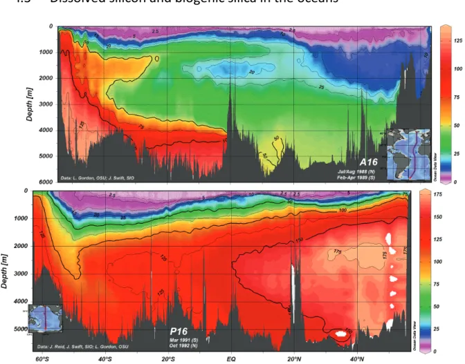
I.3 Dissolved silicon and biogenic silica in the oceans

Figure 1.2 Longitudinal section across the entire Atlantic Ocean (top panel) and Pacific Ocean (bottom panel) of the DSi concentration versus depth (eWOCE, Schlitzer, 2000).

Dissolved silicon is a major limiting nutrient in ocean for silicified organisms such as diatoms, which are a dominant phytoplankton group in the ocean (see section I.4.). Their requirement of DSi for growth (Lewin, 1962; Brzezinski et al., 1990) makes them the main actor of the marine silica cycle. The residence time for silicon in the ocean is estimated between 15 000 and 17 000 years, assuming that the silica cycle is currently at reasonably close to steady state (Tréguer and De La Rocha, 2013).

DSi is unevenly distributed in the ocean in terms of both depth and latitude (Fig 1.2). The typical depth profile shows an increase of the DSi concentration with depth. The surface ocean (euphotic zone) is affected by biological activities leading to a drop in concentration (DeMaster, 2001) to as little as a few µmol-Si L-1 in the equatorial Atlantic and Pacific Oceans (Nelson et al., 1995; Nelson and Brzezinski, 1997). In the deep ocean, DSi concentrations can reach values of 40 µmol-Si L-1 in the North Tropical Atlantic Ocean to values as high as 125 µmol-Si L-1 in the Atlantic sector of the Southern Ocean and 180 µmol-Si L-1 _{in the North Pacific Ocean (DeMaster, 2001). These high} concentrations in the deep ocean water are the consequence of BSi dissolution as it sinks through

6

inorganic dissolution in the column (DeMaster, 2001). This, coupled with the biological removal in surface waters, leads to a deep DSi concentration which is ~ 30 times higher than the surface.

However there are disparities in the deep ocean regarding the DSi concentration (Fig. 1.2). The deep ocean concentrations are the consequence of the thermohaline circulation, commonly called the Conveyor Belt, allowing for an increase of the DSi concentration during its flow by the constant settling of dissolving siliceous particles.

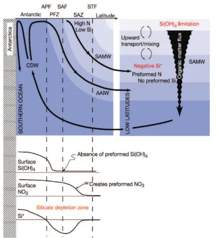
Figure 1.3 Nutrient concentrations (Si, N) from the Southern Ocean to low latitudes. Conceptual diagram depicting the Southern Ocean physical and biological processes that form low-Si* waters and feed them into the global thermocline. Water flow is depicted on top and the detail of the surface processes at the bottom. CDW: Circumpolar Deep Water, AAIW: Antarctic Intermediate Water, SAMW: Subantarctic Mode Water, APF: Antarctic Polar Front, PFZ: Polar Front Zone, SAF: Subantarctic Front, SAZ: Subantarctic Zone, STF: Subtropical Front, from Sarmiento (2004).

The transport of DSi-rich deep and intermediate waters to the surface spurs significant silica production in the regions affected. The region south of the Antarctic Polar Front, in the Antarctic Circumpolar Current (ACC) and near the Marginal Ice Zone, are the regions of the main BSi production (Fig. 1.3) due to the upwelling of deep, nutrient-rich water (Quéguiner et al., 1991; Quéguiner et al., 1997; Brzezinski et al., 2001; Fripiat et al., 2011b). In consequence, another important region for the flow of nutrient in the Atlantic Ocean is the northern part of the ACC. In the

7

subantarctic mode water, carrying nutrients to the low latitudes (Sarmiento et al., 2004). Finally the North Pacific Ocean is another region of importance where general upwelling of nutrient-rich water is observed, enriching the surface with high DSi concentrations (Sarmiento et al., 2004).

Opal rich sediments are found in various locations throughout the ocean and at all depths (from the shelf to the abyss) (Ragueneau et al., 2000). However, the Southern Ocean is the main site of opal deposition in the sediments (DeMaster, 1981). For a long time, the idea of this impressive export of biogenic silica was at odds with the idea of the Southern Ocean as a high-nutrient, low-chlorophyll area of modest productivity. Higher rates than expected for BSi production were recorded in the Southern Ocean (from 1.62 ± 0.58 mol-Si m-2 yr-1 to 3.34 ± 0.54 mol-Si m-2 yr-1 (Pondaven et al., 2000)). This resulted in a higher opal rain rate, and thus did not require exceptional preservation efficiency to explain the high rates of BSi accumulation required to maintain the "high opal belt" underlying the Polar Frontal Zone. Compared to the Atlantic Ocean, the Southern Ocean is twice as productive in term of BSi (Pondaven et al., 1998) and 2 – 3 times more productive than the Equatorial Pacific. The opal accumulation rate that leads the Southern Ocean to be the main deposit site for BSi is higher by 12 times, compared to the equatorial Pacific (0.016 mol-Si m-2 yr-1), 31 times compare with the mesotrophic northeast Atlantic (0.008 mol-Si m-2 yr-1) and by 185 times compared to the oligotrophic Atlantic (0.001 mol-Si m-2 _yr-1_).

The two processes involved in the surface and deep water, and at the surface sediment are production (P) and the dissolution (D) of the BSi (Nelson et al., 1995). These will be discussed in the next section.

I.4 Diatoms as conductors of the marine silica cycle

Diatoms are major actors of the biogeochemical cycle of silica in ocean. Diatoms are as far as we know the main silica biomineralizing group in the modern ocean; groups such as silicoflagellates, radiolarians and siliceous sponges have a comparatively smaller influence on the silica cycle. Diatoms have an absolute requirement for Si (DeMaster, 2002) and a strong affinity for DSi which means they can maintain high rates of DSi uptake (up to 0.63 µmol-Si cell-1 _d-1 _{in Martin-Jézéquel et al., 2000 and} references therein) at even very low concentrations of DSi (0.3 – 1.3 µM (Dugdale et al., 1995)). Additionally, their silicon requirement is relatively high, with a typical cellular ratio being 0.9:6.6 (mol : mol) Si:C contributing to a more efficient export of BSi compared to organic matter (Brzezinski et al., 2003). This leads to a net production of 240 Tmol-Si yr-1 _{in the surface water. In addition Baines et al.} (2012) mentioned for the first time the possible role of picocyanobacteria in the silica cycle as they

8

Synechococcus can exceed that of diatoms in some cases”.

Diatoms are also important in the biogeochemical cycles of N, P, Fe (Sarthou et al., 2005 and references therein) and have a dominant role in the export production of C (Ragueneau et al., 2000; Sarthou et al., 2005). This is due to the fact that they are numerically quite abundant and often dominate phytoplankton blooms in many aquatic ecosystems (Nelson et al., 1995; De La Rocha et al., 2000; Martin-Jézéquel et al., 2000). They account for up to 75 % of the annual primary production in the Southern Ocean (Nelson et al., 1995). 20% of the CO2 fixed during photosynthesis is the result of diatoms (Field et al., 1998). Also, very important to note, their heavy silica frustules mean they have faster sinking rates and are removed from the surface much more quickly than non-silicified cells (Smayda, 1970). For this work BSi will refer to diatoms.

I.4.1 BSi production

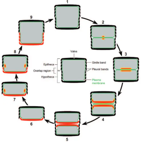
Diatoms are the main producers of biogenic silica in the marine environment. They are eukaryotic unicellular microalgae requiring dissolved silicon to produce their frustules made of amorphous, hydrated silica (opal, BSi). They have 2 modes of reproduction, a sexual reproduction involving the fusion of gametes and a vegetative mode in which silicon metabolism is strongly linked to cell division (Martin-Jézéquel et al., 2000). Here the focus will be made on the vegetative reproduction that produces an exact replica of the frustule structure at each generation.

The structure of diatoms is an outer cell wall lined internally with a plasma membrane containing the cytoplasm and organelles protected from dissolution by an organic coating. The organic matrix is made up of layers of polysaccharides, lipids and proteins. The cell wall is made of silicon dioxide (SiO2) produced through the polymerization of DSi (Martin-Jézéquel et al., 2000). The cell wall consists of 2 valves of slightly different size (Fig. 1.4), separated by a cingulum made itself of girdle bands (Kröger and Poulsen, 2008). The epitheca and hypotheca are the large and the small valve respectively. When the new mature valve is formed, the mother cell forces it out, and the mature valve is protected from dissolution by an organic coating. The creation of a new siliceous valve for the new diatom strongly links silicon metabolism and the cell cycle with restrictions due to the rigidity of the frustule (Kröger and Poulsen, 2008). As observed in figure 1.4 (7 and 8) the distance between the 2 valves increases for the new valve formation, and to avoid a gap within the cell wall the girdle bands synthesis is necessary.

The diatom cell cycle is divided in 4 phases (like every eukaryotic cell) named G1, S, G2 and M. The S phase represents the DNA replication phase, M corresponds to the mitosis and the cell division period and G1 and G2 are the gap phases during which the cell growth occurs (Martin-Jézéquel et al.,

9

observed resulting in non-continuous silicon uptake during the cell growth. There is a predominant arrest point at the G2/M boundary and another one at the G1/S boundary associated with new valve formation (Martin-Jézéquel et al., 2000). The latest can be indicative of DNA synthesis being silicon dependent but it was not proved yet and could be a way for the diatom to estimate the external Si concentration and to discern if the cell division can be completed.

Compared to nitrogen or phosphorus, the internal pool of silicon is not sufficient to support the entire division cell, therefore diatoms require Si uptake from their environment to complete their division. The Si uptake appears to regulate the DSi pool in the cell and the thickness of the frustule (Claquin et al., 2006).

Figure 1.4 Schematic structure of the diatom cell (center) and diatom cell cycle (shown in cross section). In grey: the protoplast, green line: the plasma membrane. For simplicity, intracellular organelles other than the Silica Deposition Vesicle (SDV) are not shown. Cell cycle: (1) Shortly before cell division the cell wall contains the maximum number of girdle bands, (2) immediately after cytokinesis new biosilica (red) is formed in each sibling cell inside a valve SDV (yellow), (3) expansion of the valve SDVs with increasing silica deposited, (4) at the final stage of valve SDV development, each SDV contains a fully developed valve, (5) the newly formed valves are deposited in the cleavage furrow on the surface of each protoplast by SDV exocytosis, (6) the sibling cells have separated, (7+8) expansion of the protoplast in interphase requires the synthesis of new silica (red) inside girdle band SDVs (yellow), each girdle band is synthesized in a separate SDV, and after SDV exocytosis is added to the newly formed valve (hypovalve), (9) after synthesis of the final hypovalve girdle band (pleural band) cell expansion stops, and DNA replication is initiated (Kröger and Poulsen, 2008).

10

cycle. There are the influx and the efflux of DSi from outside into the cell and inversely, the incorporation flux that allows the growth cell by BSi formation and the dissolution flux at the opposite that converts the BSi into DSi (Milligan et al., 2004). Here we will focus on the polymerisation and depolymerisation of the DSi.

I.4.2 Uptake and BSi production processes in diatom

Silicon uptake was demonstrated to occur as active transport (Paasche, 1973; Martin-Jézéquel et al., 2000 and references therein). The silicon forms available for diatom are the silicic acid at 97% (Si(OH)4) and the remaining SiO(OH)3- and the DSi influx in diatom is sodium dependent. Bhattacharyya and Volcani (1980) observed in Nitzschia alba that Si and Na+ transport is driven by the Na+ gradient across the membrane. An advantage for diatoms, that can explain their dominance in blooms, is the fact that DSi uptake is not dependant of photosynthesis energy but only from respiratory energy (Claquin et al., 2006). There are 2 pools of Si to differentiate, the intracellular silicon pool (by silicon uptake) required for silicification and the silica deposition pool (by silicon mineralization) necessary for cell division and growth (Ragueneau et al., 2000). These 2 phenomena can be coupled as in Chaetoceros gracilis, where DSi uptake and BSi mineralization occur at the same time, or uncoupled as for Thalassiosira weissflogii, depending on the species and influences the internal silicon pool (Ragueneau et al., 2000).

Silicon is transported across the plasmalemma, through the cytoplasm to reach the silicon deposit vesicle (SDV) which is located at the polymerization site (Martin-Jézéquel et al., 2000). The DSi uptake is regulated by silica transporter genes (SITs) (Hildebrand, 2008) and the deposit is regulated by proteins called silaffins (Kröger and Poulsen, 2008 and references therein). The SDV is bounded by a membrane called the silicalemma that contains an acidic environment favourable for DSi polymerisation. Proteins, cytoskeleton and some cellular components are also involved in this transformation.

The intracellular pool was observed to be in soluble form despite being at concentration supersaturated with respect to silica. Presumably some organic silicon-binding component makes this possible (Martin-Jézéquel et al., 2000 and references therein). This pool can vary depending on the species and depending on the cell stage. During cell wall synthesis, which occurs in all cycles stages G2 and M, a greater quantity of silicon will be required than can be provided by the internal pool.

Depending on DSi concentration around the cell, three modes of DSi uptake have been identified. Surge uptake consists of a rapid increase of intracellular silicon concentrations after

11

+

[

(

)

]

]

)

(

[

OH

Si

K

OH

Si

V

V

⋅

=

starvation as it is a replenishment mode. Externally controlled DSi uptake happens when the extracellular silicon concentration becomes very low and represents submaximal Si uptake rates. Finally the internally controlled uptake is regulated by use of Si in the cell, depending on the rate of Si deposit in the cell wall (Martin-Jézéquel et al., 2000).

Silicon uptake and cell division for natural assemblage or cell culture under silicon-limited conditions are well described by the following equations:

, Michaelis-Menten kinetics of nutrient uptake (1.2)

, Monod law of nutrient limited growth (1.3)

where Vmax and µmax represent the maximum rate of uptake and division at non-limiting Si concentrations, Ks is the Si concentration at 0.5 Vmax and Kµ is the silicon concentration that limits µ to 0.5 µmax (Martin-Jézéquel et al., 2000; Ragueneau et al., 2000; Claquin et al., 2006). The DSi uptake and BSi production are directly affected by environmental and physiological conditions (Passow et al., 2011) and so influence the values of KS and Vmax. It has been reported that values for KS and Vmax can evolve during the cell cycle. Low affinity and low capacity (high KS and low Vmax) were observed for Si uptake by Navicula pelliculosa before frustule deposition but the opposite during the deposition of BSi. The explanation advanced for the KS decrease is higher affinity transporters and for the increase of Vmax it is a bigger number of transporters or a better efficiency of these latter in the plasma membrane (Martin-Jézéquel et al., 2000 and references therein).

Environmental conditions will have an effect on the growth rate of diatoms, mainly through co-limitation. For example Brzezinski et al. (2008) demonstrated that addition of iron in the environment significantly increases Si uptake by 87 ± 59 %, but that addition of Fe and Si increases the uptake up to 172 ± 43 %. This study revealed a co-limitation Fe - Si. Another co-limitation, between Fe and light was highlighted by Sunda and Huntsman (1997). This study revealed that in low light environments, diatoms are more iron limited, these conditions stimulate the development of small cells.

A decoupling exists between silicon metabolism and photosynthesis that is species dependent (Ragueneau et al., 2000). In 1955 Lewin indicated that the energy needed for silicification comes from aerobic respiration. Energy is required for silicon transport but there is not really a need of energy for biogenic silica mineralization, outside of what is necessary to create the organic matrix that guides polymerization of the silica (literature review in Martin-Jézéquel et al., 2000). For example, Sullivan (1986), described that after an increase in respiration with a period of silicon

]

)

(

[

]

)

(

[

OH

Si

K

OH

Si

+

⋅

=

µ

µ

12

between silicification and photosynthesis could explain why Si uptake and deposit can happen in the dark (Martin-Jézéquel et al., 2000). And knowing that carbon and nitrogen uptake are directly dependent on photosynthetic energy while silicon is dependent on the respiration of general cellular stores of energy, this can explain diatom dominance in phytoplankton blooms. Indeed, under less favourable conditions (i.e. water column mixing following a storm even) that could deepen the Mixed Layer, and so increase the depth at which they can “stay” (limit of the euphotic zone) they are more adapted to growth. Moreover diatoms have higher growth rates than dinoflagellates explaining why they bloom.

The advantages of having a frustule still remain unclear but some hypotheses are made. One major hypothesis is the protective role of the frustule against grazing by zooplankton. It was confirmed that because of the huge pressure needed to break the frustules, this is a good protection and that could explain the success of diatoms by decreasing their mortality rate (Hamm et al., 2003; Smetacek et al., 2004). Other assumptions are made about a possible role as an ultraviolet filter (Davidson et al., 1994), as a photonic crystal (Fuhrmann et al., 2004) or as ballast to control the position of diatom cells in the water column (Villareal, 1988). According to (Raven, 1983) there is less cost in creating a cell wall made of BSi rather than organic carbon. And lately, the role of polymerized silica as a buffer for the carbonic anhydrase (catalyser of the reaction between HCO3- and CO2) was demonstrated by Milligan and Morel (2002).

I.4.3 Silicon dissolution and export

The second process affecting silicon in the marine environment is the dissolution of biogenic silica between a few hundred meters from the surface (Passow et al., 2003) and to the sediments (Van Cappellen et al., 2002). The dissolution (at neutral pH) is due to nucleophilic attack of water molecules that breaks Si-O-Si bonds found at the surface of the frustules (Loucaides and Behrends, 2008). The BSi dissolution rate determines the fraction of silica recycled in the euphotic zone that contributes to the gross amount of silicic acid that is available for diatom growth each year. The fraction recycled at depth (Passow et al., 2003) controls silicon recycling in the oceans (Van Cappellen et al., 2002) versus its burial in deep sea sediments and export from the ocean. Recycling and export of silicon are linked to areas of significant diatom productivity. The residence time of the BSi in the surface layer depends on the sinking speed and the dissolution rate. Seasonality, food web structure and aggregate formation are the main processes that will impact the export of silica (Ragueneau et al., 2000). According to Nelson et al. (1995), 50 to 60 % of the marine BSi produced dissolves in the euphotic zone and less than 3 % is buried in the sediment (DeMaster, 2001). But the export rates are

13

the ocean (surface < 50 µM DSi, deep < 180 µM DSi) (Tréguer et al., 1995; Passow et al., 2003). Frustules of living diatoms are protected from dissolution by an organic coating that isolates the cell from the slightly basic pH of seawater. In living diatoms the dissolution rate is minimal (0.2 to 0.3 % d-1) unless bacteria have colonized the cells (Bidle and Azam, 1999). Dissolution begins when diatoms die, as bacteria start to degrade this protection around the frustules letting the BSi underneath come into contact with seawater resulting in high dissolution rates of BSi in the upper ocean (Passow et al., 2003). Hurd and Birdwhistell (1983) described the specific dissolution rate Vdiss (h-1_{) of the BSi as follow:}

, (1.4)

where k is a constant (cm h-1), Si(OH)4sat is opal solubility (mol cm-3), Si(OH)4 is the ambient DSi concentration (mol cm-3_{) and A}

sp is the specific surface area of opal present (cm² mol-1). This equation allows us to better understand the conditions affecting the dissolution rate in the ocean, for example allowing us to discern that the lowest dissolution rates occur in the Antarctic between – 1.5 °C and + 6 °C and the highest dissolution rates occur in coastal waters between + 14 °C to + 22 °C. These observations led to the conclusion that the temperature of the surface layer plays an important role in the dissolution rate observed in different regions.

From experiments a list of physical and chemical processes that modify dissolution has been made. An increase of the temperature or pH will have increased the dissolution rate, while silica with a greater aluminium content or otherwise impurity will inversely decrease the dissolution rate. A pH increase leads to a deprotonation of Si-OH groups at the surface, facilitating then the Si-O-Si bounds to be broken (Loucaides and Behrends, 2008). The composition of the cell medium, the morphology and the structure of the frustule more than the surface area (Martin-Jézéquel et al., 2000) and the silica's age will as well influence dissolution (Van Cappellen et al., 2002 and references therein).

Food web structure impacts recycling and export of BSi by grazers that feed on diatoms. Grazing by heterotrophic dinoflagellates will remove all organic matter from the frustules, leaving them exposed to seawater, and so increase the dissolution rate of the silica. Grazing by crustaceans like copepods will have two different effects. The first effect is to break the frustules into smaller pieces in surface waters, inhibiting their export from the surface (Ragueneau et al., 2006). The second is to export BSi via fecal pellets (Beucher et al., 2004), contributing to the export of the silica to the deep ocean. Diatoms may also sediment as aggregates. Aggregation can play a protection role if there is

sp sat

diss

k

Si

OH

Si

OH

A

14

of dissolution if there is considerable bacterial activity in the aggregate (Passow et al., 2003).

I.4.4 BSi as a proxy

We have just seen that diatoms are the main actor of the silica cycle, that the DSi concentration influences diatom growth and that 3% of the BSi produced in surface waters reaches the seafloor. There has been strong interest in using the BSi that accumulates in the sediment to somehow reconstruct the productivity of the past ocean. De La Rocha et al. (1997) suggested that the silicon isotopic composition of this silica might serve as a robust proxy for the extent of utilization of DSi by diatoms. They showed that diatoms fractionate Si isotopes in favour of the light isotope (28_{Si) when} they take up DSi to produce BSi, leading to BSi lower by 1.1 ± 0.4 ‰ compared to the DSi source. This fractionation was not observed to vary with temperature (in the range 12 – 22 °C) nor among the three species of diatoms tested. However this year Sutton et al. (2013) revealed fractionation during BSi production being species dependant. The extremes values obtained were for two Southern Ocean diatoms, Fragilariopsis kerguelensis and Chaetoceros brevis that expressed fractionation of – 0.54 ‰ and –2.09 ‰. The previous value defined by De La Rocha et al. (1997) is in the range of these values. In 2009 Demarest et al. observed fractionation again in favour of the light isotope during BSi dissolution leading to the production of DSi lighter by 0.55 ‰ compare to the BSi.

II Isotope systematics

II.1 The silicon isotope system

Atoms of the same element, with the same number of protons (Z) and electrons but with different numbers of neutrons (N) are called isotopes. Because they do not have the same number of neutrons, all isotopes of an element have a different atomic masse (m). The atomic mass variations of an element leads to small differences in chemical and physical properties, known as isotope effects (Hoefs, 1996). Stable isotopes are defined as nuclides with low atomic mass and with a stability achieved when the number of protons and neutrons are approximately equal. The process resulting in variation of abundance of isotopes is called fractionation. Processes that induce isotopic fractionation cause differences in the ratios of the different isotopes of an element between two substances or between two phases of a substance.

Hoefs (1996) highlighted the existence of two types of mass-dependent fractionation laws. There is kinetic isotopic fractionation that results from motions and unidirectional reactions, and

15

or two phases, and that is bidirectional. The extent of mass dependent fractionation by a kinetic isotope effect is very slightly different from that of an equilibrium isotope effect, allowing the two to be distinguished in a set of extremely precisely measured samples. The resulting slope of the silicon isotopic composition of samples on a three isotope plot (i.e. δ29_{Si versus δ}30

Si) is either 1.93 or 1.96, corresponding to kinetic or equilibrium isotope fractionation respectively (Young et al., 2002).

Silicon has three natural stable isotopes, 28Si, 29Si and 30Si, for which the relative abundance is respectively 92.22 %, 4.69 % and 3.09 %. There is also a radioactive isotope 32Si with a half life of 140 ± 6 years. The relative mass difference between the heaviest and the lightest isotopes (30_Si/28_{Si = 7} and 29Si/28Si = 3.6) indicate that large mass-dependent fractionations are to be expected (Engström, 2009). The isotope ratio variations are expressed as δ29Si or δ30Si as follows:

‰, (1.5)

where x corresponds to 29Si or 30Si. The standard (std) commonly used is the international Si standard NBS28 (RM8546).

The measurement of silicon isotopes is interesting due to silicon abundance, for example, silica represents ~ 60 % of the dry weight of diatoms (Sicko-Goad et al., 1984). Moreover, in the Southern Ocean, an ocean of importance for the distribution of nutrients in the ocean, the seafloor is rich in opal and poor in carbonate. Douthitt (1982) made the first observation of a difference in the natural abundance of Si isotopes in diatoms compared to igneous rock.

II.2 Silicon isotopes in different environments

Variations in silicon isotopes offer a means to track processes involving silicon utilisation and fractionation. The weak valence of silicon (4+) is bound with O and the non-existence of a gaseous phase leads to little isotopic fractionation on Earth. The four domains in which silicon fractionation is involved are rock-forming, water-rock interactions, biological processes and water reservoirs. I will focus on the water-rock interactions, rivers and oceanic biological processes that are more relevant for this study.

1000 1 28 28 ⋅               −         = std x sample x x Si Si Si Si Si

δ

17

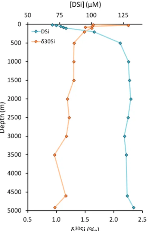
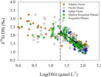
SiDSi mainly due to biological activities, and due to BSi dissolution and the circulation and mixing of water masses. Because diatoms that are in the euphotic zone take up DSi to build their frustules, a gradient with depth is observed with δ30

SiDSi decreasing with depth as DSi concentrations increase. The highest marine values of δ30_Si

DSi are found in surface waters with a maximum value of + 3.10 ‰ recorded by Varela et al. (2004) in the Pacific sector of the Southern Ocean. For the deep water (> 2000 m) average values are + 1.20 ‰ for the Antarctic Circumpolar Current (Fripiat et al., 2011a) and + 1.25 ‰ for the deep water of equatorial Pacific Ocean and Pacific sector of the Southern Ocean (de Souza et al., 2012a). A typical silicon isotopic profile is presented in figure 1.6.

Figure 1.6 Typical profile of δ30

SiDSi and DSi concentration versus depth in marine environment (data from

this PhD). Blue diamonds are δ30

SiDSi values and orange diamonds are the corresponding DSi concentrations.

To estimate the fractionation between the DSi used and the resulting BSi by diatom based on the evolution of silicon isotopes in surface waters during DSi drawdown, either of the two simple models can be used. The fact that these models only work during times of net nutrient drawdown is a key point, as this makes them unsuitable for use at other times. Not all production of biomass in the ocean occurs during times of net nutrient removal (i.e. there are times when net production of biomass occurs but does not exceed daily inputs of nutrients to the euphotic zone through upwelling or mixing).

The Rayleigh distillation (or closed system) model (Fig. 1.7, eq. 1.6) (De La Rocha et al., 1997; Sigman et al., 1999) assumes a single input of nutrient to the surface at the beginning of the growing

18

season, that the reservoir is well mixed and that the BSi produced does not subsequently dissolve or exchange isotopes with the remaining DSi reservoir:

    ⋅ + = initial measured DSiinitial DSi _DSi DSi Si Si ] [ ] [ ln 30 30 δ ε δ (1.6)

It is characterized by an exponential enrichment of DSi reservoir through time with BSi formation and accumulation of the product formed.

Figure 1.7 Representation of the Rayleigh distillation model (solid lines) and the Steady state model (dotted lines). ƒ: remaining fraction, blue: DSi, green: BSi and grey: BSi accumulation in the system.

The second model is the Continous input model (or open model) (eq. 1.7) (Sigman et al., 1999). This model hypothesizes a continuous input of DSi to the surface over the growing season. DSi is partially consumed and the residual fraction exported:





















−

⋅

−

=

_DSi

DSi

Si

Si

]

[

]

[

1

δ

ε

δ

BSi deposits in the sediment have an important role in helping us to determine the patterns and controls over past climate. Diatoms make an important contribution to primary production in the Southern Ocean and because primary production is CO2 consuming, there is a great interest of using opal in the sediment to reconstruct diatom productivity in relation to past climate. A reconstruction based only on the rate of sediment deposition is complicated by the fact that 50 % of the BSi produced is dissolved in the first hundred meters and ocean circulation leads to the deposition of BSi not necessarily in the area of its production. To counteract that, De La Rocha et al., (1998) used the silicon isotopic composition of the BSi as a proxy. This suggested that during the Last Glacial Maximum (Fig. 1.8 arrow) the extent of DSi utilisation was smaller than today (and coincided with reduced rates of opal accumulation on the seafloor). The opposite was true for the Holocene. A study

20

that helps to place the data chapters into a broader context. The 2nd chapter describes the methods used for the collection and analyses of samples. Chapter 3 is the publication “Exploring interacting influences on the silicon isotopic composition of the surface ocean: a case study from the Kerguelen Plateau”. The 4th chapter is composed of a first part that is a general overview of the intermediate and deep circulation in the Atlantic Ocean. This is a background followed by the second part which describes the silicon isotopes data in the Atlantic Ocean, as part of the GEOTRACES Zero and Drake transects, the ANTXXIV/3 campaign and the MSM10/1 campaign. This thesis ends with general conclusions as the 5th _chapter.

23

Chapter 2 – Methods and analytical

techniques

This chapter presents the steps used in the preparation of samples detailed in the following chapters and the measurement of isotope ratios with the multi-collector inductive coupled plasma mass spectrometer (MC-ICP-MS) Neptune (Thermo Fisher Scientific). The initial collection of samples in the field is detailed in the chapter specific to each oceanographic campaign.

I Sample preparation

I.1 Determination of DSi concentration

The first step in the preparation of samples for mass spectrometry was the determination of the dissolved silicon (DSi) concentration of the samples. The well known interaction between silicic acid and molybdate was used to determine the concentrations colorimetrically with a spectrophotometer (Shimadzu UV-1700) following the formation of a complex of silicomolybdate (H4SiMo12O40) and its reduction to create a blue solution (Strickland and Parsons, 1972). This technique allows only the dissolved, monomeric form of silica and straight-chain polymers of relatively short length to react with molybdate. However, even polymers at low DSi concentrations are not a problem for DSi concentration determination due to the fact they are “probably unreactive”, as described by the authors.

The ammonium molybdate ((NH4)6Mo7O24 · 4H2O) reagent was prepared with concentrated HCl and stored in a polyethylene bottle. The reducing agent was a mix of metol-sulphite (Na2SO3 + (C7H10NO)2SO4), sulphuric acid (H2SO4) and saturated oxalic acid (C2H2O4) stored in polyethylene bottles. For a sample 2 mL metol-sulfite + 1.6 mL Milli-Q water + 1.2 mL of 50% H2SO4 + 1.2 mL of saturated oxalic acid are needed. All acids used are analytical grade and diluted with Milli-Q water (18.2 MΩ cm-1

).

For the standard curve a minimum of 7 concentrations were used in clean polyethylene bottles ranging from 0 µmol-Si L-1 (blank) to 140 µmol-Si L-1 (133 µmol-Si L-1 was the maximum concentration measured) covering the DSi concentration range of samples. Artificial seawater prepared according to Strickland and Parsons (1972) was used to match our samples, and the silica standard used was silicon hexafluoride (SiF62-).

The blank was prepared by mixing the reducing agent with artificial seawater. Straight after that addition the reagent is poured and mixed. The standard solutions and samples were prepared by

24

reagent plus sample and mixed in the bottles. Approximately three hours is needed for the reaction to stabilise before the measurements are performed at a wave length (λ) of 810 nm.

I.2 Magnesium induced coprecipitation (MAGIC)

The samples were preconcentrated according to an adapted brucite coprecipitation (MAGIC) technique developed by Karl and Tien (1992). The principle is to add sodium hydroxide (NaOH) to a seawater sample to reach a pH ≥ 10 which will induce the precipitation of the brucite (Mg(OH)2) and many solutes including DSi. To initiate the precipitation, 2 % volume of 1 M NaOH is added to the samples and mixed. Another centrifugation was performed one hour later and the precipitates from the two centrifugations are added to the same sample and dissolved in concentrated HCl for recovery of DSi. This was found necessary for complete recovery (i.e. 97.93 %) and quantitative extraction of DSi from seawater.

I.3 Tri-ethylamine molybdate coprecipitation (TEA-moly)

DSi quantitatively reacts with the molybdate ion at acidic pHs, allowing a DSi extraction from seawater and purification via precipitation of the silicomolybdate ion, as triethylamine silicomolybdate (DeFritas et al., 1991; De La Rocha et al., 1996). This method permits quantitative recovery of silicon even for samples with low concentration (10 µM). Quantitative recovery is very important to avoid silicon fractionation during silicon extraction that can occur if an isotope is preferentially removed compared to other silicon isotopes. Following the protocols of De La Rocha et al. (1996), the prepared reagent stands for seven days in a dark polyethylene bottle to let the trace amounts of silicon in the water and/or reagents to precipitate as triethylamine silicomolybdate. The reagent is prepared by mixing ammonium molybdate ((NH4)6Mo7O24 · 4H2O) and tri-ethylamine hydrochloride ((C2H5)3N · HCl). When the trace amounts of silicon have precipitated, the reagent is filtered through a 0.4 µm polycarbonate filter immediately prior to use (Fig. 2.1). For each 100 mL of water sample, 60 mL of reagent was added.

The coprecipitation reaction occurs in two steps. Firstly, monomeric Si(OH)4 reacts with molybdate to form silicomolybdic acid (H4SiO4 · 12MoO3), and then silicomolybdate reacts with triethylamine to form an insoluble, yellow complex, triethylamine silicomolybdate (((CH3CH2)3NH)4SiMo12O40 · 4H2O). The pH must be acidic (between 1 and 4) and the DSi concentration must be > 3 µM-Si for the reaction to proceed rapidly and quantitatively. Once the complex is formed, the sample is given 24 h for complete reaction before filtration through a 0.4 µm

26

with HF charges the silicon negatively (anion) as SiF62-, and therefore, an AG 1-X8 strong base anion exchange resin (BioRad or Eichrom) was used. This resin is a polymer of fixed ion as N-CH2N-(CH3)3 linked with an ion that is mobile (e.g., Cl-_{). The particle size of the resin used was 100 ─ 200 mesh} (150 ─ 75 µm). The resin beds of ~1.8 mL were placed in acid-cleaned columns of 2 mL (Eichrom) and held in place by a frit at the bottom and at the top of the resin bed.

The resin is first washed using Milli-Q water and then preconditioned with 15 mL of 2 M NaOH. 7.7 mL of sample, containing 4 µmol-Si and having a HF concentration of 52 mM, is loaded into the column. The ions of SiF62- are retained on the resin, displacing the OH- carried by NaOH. The sample matrix (including potential contaminants) is eluted using Milli-Q water followed by a solution of 95 mM HCl + 23 mM HF and another of 23 mM HF. To elute the Si from the column, two 10 mL aliquots of 0.14 M HNO3 + 5.6 mM were used, with the second being collected as it contains all of the Si loaded onto the column (i.e., 99.34 ± 0.20 %). The concentration of purified Si in the eluent was thus 11.2 ppm of Si. During each session, a blank of 52 mM HF was run on a column that is silica clean at 99.62 ± 0.16 %. A minimum of one silica standard was also run on one column during each session. The silica standard commonly used is the NBS28 (RM8546), a quartz sand sample supplied by the National Institute of Standards and Technology (NIST). Another silica standard used was a 99.995 % pure silica sample (Alfa Aesar) adopted as the working standard (De La Rocha, 2002). Samples, blanks and standards were stored in acid-cleaned polypropylene centrifuge tubes (VWR) in the clean lab until analysis on the mass spectrometer.

II Mass Spectrometry

The mass spectrometry method is the most effective way to determine atomic and molecular masses and isotope abundance of a sample. In a mass spectrometer the sample is converted into an ionised, gaseous state, and charged molecules or charged atoms are separated according to their mass to charge (m/z) ratio, and their relative abundance is recorded.

II.1 Sample dilution

As mentioned in the chapter 1, silicon has three natural stable isotopes, 28Si, 29Si and 30Si, for which the relative abundance is respectively 92.22 %, 4.69 % and 3.09 %. The silica samples are diluted from 1.5 to 2.5 ppm to obtain a signal of ~10 V on the mass 28, at medium resolution. The samples and standards were matched for silicon and acid concentrations to obtain the same signal. A sample-standard bracketing technique was used, that required identical solutions to avoid a

matrix-27

standards are “spiked” with an external element, which is chosen according to its mass being as close as possible to the targeted element (See section II.3.2.). For silicon (28Si, 29Si and 30Si) the most suitable element is magnesium due to its isotopes 24_Mg, 25_{Mg and} 26_{Mg. We used a pure} mono-elementary Mg solution (Cardinal et al., 2003).

II.2 Multi-Collector - Inductive Coupled Plasma Mass Spectrometry

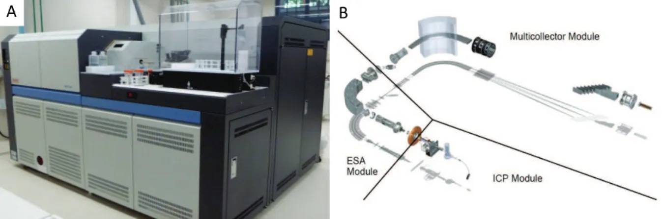
The Neptune (Thermo Fisher Scientific, Fig. 2.2 A) is a double-focusing mass spectrometer used for the analyses at Ifremer (Brest, France). It is divided in three main parts, the inductively coupled plasma module (ICP), the electrostatic analyser module (ESA) and the multi-collector module (Fig. 2.2 B).

Figure 2.2 A) Neptune (Thermo Fisher Scientific), B) Main parts of the Neptune, the Inductively Coupled Plasma module (ICP Module), the Electrostatic Analyzer module (ESA Module) and the Multi-collector module (wwz.ifremer.fr/Neptune).

The ICP module is composed of the inlet system and the plasma where the sample is ionised. The inlet system conveys the liquid sample via aspiration from the sample vial, generally positioned in an auto-sampling rack, into the nebulizer, where the sample is transformed into a fine aerosol by argon (Ar) gas flowing through the nebulizer. In general, this mist enters in the spray chamber that prevents large droplets from passing through to the plasma. However, during this study a desolvating nebulizer (for earlier measurement (samples from ANTXXIII/9) the Apex was used, and for later measurements (ANTXXIV/3 and MSM10/1) the Aridus II) to minimise the transfer of all liquid to the plasma. Carried along by a flow of Ar gas, the sample reaches the torch where it is injected into the plasma and ionised. The Ar plasma is maintained by a coupling coil which transmits a specific radio frequency to the heated Ar gas which is ignited by a spark. The plasma is extremely hot, especially towards its core, and the sample is ionised upon contact with it.

28

atmospheric pressure into a 10-6 Torr pressure mass spectrometer. The aim is to reduce ion dispersion by filtering the speed and energy of the ions transmitted and to accelerate them through the system. This helps to obtain a peak shape with a flat top needed for precise, accurate, and stable measurements of isotope abundance ratios. For that, immediately after ionisation of the sample in the plasma, the ions go through a sampler cone which blocks all ions except for those travelling with a directly forward trajectory at the centre of the plasma. After passing through the small orifice of the sampler cone, the ions spread out and are subsampled again a few centimetres later by the skimmer cone, which is steeper and has a smaller orifice. Again, only the ions at the centre of the ion beam pass through the skimmer cone. This allows a uniform ion beam and a decrease in pressure moving in to the high vacuum area of the mass spectrometer. Through the lens system that is downstream of the cones, the vacuum starts to improve and the ions begin to accelerate towards the Faraday detectors due to the electrical field established in the mass spectrometer. When the ion beam reaches the electrostatic sector, the ions are diverted according to their energy to the magnetic sector. The electrostatic sector is composed of two curved plates with direct current voltages that have opposite polarity, attracting oppositely charged ions thus creating ion aversion. The ion beam is focused and deflected with a 90° angle and an intermediate slit at the end of the ESA acts as an energetic filter allowing only ions with a narrow range of kinetic energy to pass.

The multi-collector module is where the mass separation and detection of ions take place. This consists of the magnetic sector that separates ions into beams characterised by their mass to charge value. After the magnetic field each separated ion beams is collected by one of the eight available Faradays cups, four on the low mass side (L4, L3, L2, and L1) of a fixed central cup (C), and four on the high mass side of the central cup (H1, H2, H3 and H4). For Si masses 28, 29 and 30, the cups used are L2, C and H2. Ions landing in a cup are transformed into an electrical impulse which is amplified to give an ion current proportional to the isotope abundance.

II.3 Performance of a MC-ICP MS

There are potentially three types of errors/problems that can occur during analyses of silicon isotopes when using the mass spectrometer: (1) interferences with the masses of interest (28, 29 and 30 in this study), (2) overestimation of sample peak intensities due to high blank concentrations, and (3) isotopic fractionation at the interface part of the machine (De La Rocha, 2002; Cardinal et al., 2003; Engström et al., 2006).

Three procedure blanks are used for correction for each run on the Neptune. A procedure blank has the same composition and concentration of acid as the sample and standard, and goes through

29

three procedure blanks are measured for each silicon isotope and used to correct measurements on the mass spectrometer by subtracting the blank average from the isotope value measured. The operating conditions of the Neptune are described in Table 2.1

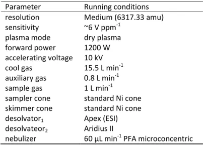
Table 2.1 Characteristics of the MC-ICPMS Neptune (Ifremer, Brest) used for the silicon isotopes measurements.

II.3.1 Mass interferences

The interferences due to nickel (58Ni2+, 60Ni2+) and iron (56Fe2+, 58Fe2+) are eliminated by the column chromatography chemistry because they can create interferences by forming doubly charged ions located at the same m/z values as silicon isotopes (Engström et al., 2006). Isobaric interferences such as from compounds containing carbon, nitrogen and/or oxygen and hydrides (28SiH+ and 29SiH+), that are an unavoidable by-product of ionisation in a plasma, are avoided by the resolution performance of the Neptune (Engström et al., 2006). The resolution of the machine is its ability to separate masses at the entrance slit and can be set to low, medium or high. Improvement of the resolution allows a better separation of the masses but leads to a decrease in the signal,and therefore, the medium resolution was the best compromise for our analyses. The resolving power (resolution: R) for a multi-collector mass spectrometer is calculated according to Weyer and Schwieters (2003) as follows: m m R ∆ = , (2.1)

where m is the mass of the isotope (30 for silicon) and Δm is the difference between 5 and 95% of the mass intensity signal. An average R of 6317.33 atomic mass unit (amu) was obtained at medium resolution during this study.

Parameter Running conditions

resolution Medium (6317.33 amu) sensitivity ~6 V ppm-1

plasma mode dry plasma

forward power 1200 W

accelerating voltage 10 kV cool gas 15.5 L min-1 auxiliary gas 0.8 L min-1 sample gas 1 L min-1

sampler cone standard Ni cone skimmer cone standard Ni cone desolvator1

desolvateor2

Apex (ESI) Aridius II