Academic and Research Staff Prof. H. L. Van Trees Prof. D. L. Snyder
Graduate Students
M. E. Austin L. D. Collins R. R. Kurth
A. B. Baggeroer T. J. Cruise A. P. Tripp, Jr.
RESEARCH OBJECTIVES AND SUMMARY OF RESEARCH The work of this group may be divided into four major areas. 1. Sonar
The central problem of interest is the development of effective processing techniques for the output of an array with a large number of sensors. Some specific topics of
interest in this connection are the following.
(i) A state-variable formulation for the waveform estimation problem when the signal is a sample function from a possibly nonstationary random process that has passed through a dispersive medium before arriving at the array. Some preliminary results
have been obtained. 1
(ii) The effects of array velocity on the system performance when operating in a reverberation-limited environment.2
(iii) Iterative techniques to measure the interfering noise field and modify the pro-cessor to reduce its effect.
(iv) A hardware-efficient analog transversal equalizer has been designed, and the basic components built and tested. With some additional work, a completed transversal filter will enable us to apply actual channel measurements to its time-variable tap gains, thus making possible laboratory simulations of dispersive channels. Such simulations are expected to provide a convenient means of evaluating channel parameter estimation techniques, and to prove useful in the development of better models of the sonar channel. 2. Communications
a. Digital Systems
Decision-feedback systems offer an effective method for improving digital commun-ications over dispersive channels. A new structure has been derived whose performance should be appreciably better than previous systems. Theoretical work on this decision-feedback scheme will continue; it will be viewed as an integral part of an adaptive
receiver whose acquisition and tracking behavior are of interest in equalization of dis-persive channels. The analog transversal filter that is being constructed as a channel-measuring and channel-simulation device (see (iv) above) will also prove useful in evaluating the performance of algorithms that have been developed for adjusting the parameters of these adaptive receivers.
*This work was supported by the Joint Services Electronics Programs (U. S. Army, U. S. Navy, and U. S. Air Force) under Contract DA 36-039-AMC-03200(E)).
(XXVII. DETECTION AND ESTIMATION THEORY)
The optimum receiver for the detection of Gaussian signals in Gaussian noise is well known. Except for limiting cases it is difficult to evaluate the error behavior. Work con-tinues on developing performance measures for evaluating the performance, emphasizing techniques that are computationally tractable and, at the same time, give a good meas-ure of the system performance. Both tight upper bounds and computational algorithms have been developed for the probability of error which emphasize the fundamental role of optimum linear systems in detection problems. Future work includes the application of these techniques to the analysis and design of radar, sonar, and communication sys-tems.
The availability of a noiseless feedback channel from receiver-to-transmitter enables a significant increase in performance. By utilizing the continuous feedback signal at the modulator, the behavior system performance at the end of the transmission interval is greatly improved. The feedback link could be used to obtain the same performance over a shorter transmission interval. The actual structure of the system is very flexible and simple.
Noise in the feedback channel degrades the achievable system performance with the simple feedback system. Improvement over the no-feedback system is obtained, but it is not as dramatic as when noiseless feedback is available.
b. Analog Systems
(i) Investigations of the performance of analog modulation systems operating in addi-tive noise channels are essentially completed.3
(ii) When a noiseless feedback link is available from receiver-to-transmitter simple modulation schemes can be developed which achieve the rate-distortion bound. Realizible feedback systems perform very close to the rate-distortion bound.
The effects of additive noise in the feedback link depend on the relative noise levels in the two channels. For relatively small feedback channel noise, the system performance is close to the rate-distortion bound. For large feedback noise the availability of a feed-back link does not significantly improve the system performance.
(iii) A new approach has been developed for estimating continuous waveforms in real time. The approach is formulated with continuous Markov processes and use is made of state-variable concepts. The approach has been applied successfully to the problem of estimating continuous stochastic messages transmitted by various linear and nonlinear modulation techniques over continuous random channels; particular emphasis has been given to phase and frequency modulation. An advantage of this approach over alternative
schemes is that it leads automatically to physically realizable demodulators that can be readily implemented.4
3. Seismic
A substantial portion of our effort in this area is devoted to acquiring an adequate understanding of geophysics in order to formulate meaningful problems. An area of concentration is exploration seismology in land and ocean environments. Some specific problems of interest include array design and effective quantization techniques.
4. Random Process Theory and Application
a. State-Variable and Continuous Markov Process Techniques
(i) In the theory of signal detection and estimation, it is frequently of interest to determine the solutions to a Fredholm integral equation. A state-variable approach to the problem of determining the eigenfunctions and eigenvalues associated with the prob-lem has been formulated.
The random process(es) is represented as the output of a linear dynamic system that is described by a state equation. The Fredholm integral equation is reduced to a vector differential equation that is directly related to the state equation of the dynamic system. From this equation, a determinant is found which must vanish in order that an eigenvalue exist. Once the eigenvalue is found, the eigenfunction follows from the transition matrix of the vector differential equation.
The technique is general enough to handle a large class of problems. Constant-parameter (possibly nonstationary) dynamic systems for both scalar and vector processes can be handled in a straightforward and analytic manner. Time-varying systems can also be treated by computational techniques.5
(ii) The problem of formulating a state-variable model for random channels encoun-tered in practice is being investigated. A particular class of channels of interest are those exhibiting frequency-selective fading.
(iii) The system identification problem is being studied. Applications include meas-urement of noise fields, random process statistics, and linear system functions.
b. Detection Techniques
Various extensions of the conventional detection problem to include nonparametric techniques, sequential tests, and adaptive systems are being studied.
H. L. Van Trees References
1. A. Baggeroer, "MAP State-Variable Estimation in a Dispersive Environment," Internal Memorandum, December 10, 1966 (unpublished).
2. A. P. Tripp, Jr., "Effects of Array Velocity on Sonar Array Performance," , S. M. Thesis, Department of Electrical Engineering, M. I. T. , 1966.
3. T. L. Rachel, "Optimum F. M. System Performance - An Investigation Employing Digital Simulation Techniques," S. M. Thesis, Department of Electrical Engineering, M. I. T. , 1966.
4. D. L. Snyder, "The State-Variable Approach to Continuous Estimation," Ph.D. Thesis, Department of Electrical Engineering, M. I. T. , 1966.
5. A. B. Baggeroer, "A State-Variable Technique for the Solution of Fredholm Integral Equation" (submitted to IEEE Transactions on Information Theory).
A. EQUALIZATION OF DISPERSIVE CHANNELS USING DECISION FEEDBACK 1. Introduction
Several authors have recently considered decision feedback as a means of improving digital communication over dispersive channels. Lucky1 applied decision feedback to the equalization of telephone lines, effectively enabling him to achieve dispersion meas-urements via the message sequence, rather than having to send additional signals to
"sound" the channel before information transmission. Aein and Hancock2 have analyzed the performance of a nonlinear decision-feedback receiver, applicable to channels in which the dispersion is restricted to less than two baud durations. Drouilhet and
(XXVII. DETECTION AND ESTIMATION THEORY)
Neissen3 have studied and are constructing a decision-feedback equalizer, differing from that of Lucky in that they use a matched-filter ahead of their equalization filter, and use decision feedback to "subtract out" the effects of the message in order to improve their continuous, "sounding-signal" channel measurement.
The equalizer structure considered by Lucky is the conventional tapped delay line (TDL), which has long been used in correcting telephone lines, while Drouilhet and Niessen are using the MF-TDL structure, arrived at through different approaches and
criteria by several persons (for example, Tufts,4 George, 5 and Austin6). Both efforts are examples of how decision feedback has been used to facilitate channel measurement and the adjustment of parameters of what we shall refer to henceforth as "conventional" equalizers. We shall show in this report that decision feedback can be used to addi-tional advantage in channel equalization, if one adopts the new equalizer structure developed in the sequel, hereafter referred to as the "decision-feedback" equalizer to
distinguish it from the conventional equalizers mentioned above.
We want to consider the problem of determining the structure of a receiver for digital communication over a linear dispersive channel whose equivalent impulse
response, h(t), is known. The receiver input is
00
r(t) = kh(t-kTb) + n(t), (1)
k=-oo
where Tb is the baud duration, and k contains the information transmitted on the
th
k baud. Our problem is to decide between the hypothesis H that
to
= +1 and hypothesis H1 thatto
= -1. We make the following assumptions.(i) The ek are independent. (ii) Ho and H1 are equally likely.
(iii) n(t) is white Gaussian noise, Rn(T) = ().
At this point we would like to derive the optimal receiver structure, assuming only that k = +1 or -1 on each baud. This, however, proves analytically intractable, and therefore we shall adopt an approach leading to a suboptimal receiver structure, which nonetheless exhibits definite advantages over existing conventional equalizer structures. This requires us to make additional assumptions.
(iv) The k are N(O, o) for k > 0. (v) The k are known for k < 0.
We note that assumption (iv) renders our model inaccurate for binary AM or PSK systems in which k = +1 or -1 for all k, while assumption (v) is only valid for decision-feedback equalizers in the absence of decision errors.
(Fig. XXVII-4); then we shall optimize its parameters for the binary communication problem of interest (Eqs. 5 and 6). Finally, we shall work a simple example demon-strating that our new decision-feedback equalizer is capable of rendering far better per-formance than the conventional MF-TDL receiver.
2. Structure of the Decision-Feedback Equalizer
We want to determine the optimum receiver structure for the problem and assumptions that have been introduced, but first we introduce some notation and definitions that will prove useful in the derivation that is to follow.
Definitions:
1.
-_
=
{( kk<0}
2. + = k jk>0} 3. ak 1 r(t) h(t-kTb) dt r(t+kTb) h(t) dt O o 4. bk = h(t) h(t-kTb) dt. oUnder our assumptions, - is known correctly via decision feedback, and with this taken into account, the optimum receiver calculates the likelihood ratio
p[r(t) Ho p[ r(t) H, o, +i(P ) di
p [r(t) , H1 p[r(t), ;1, p(6 ) d
We shall first consider the numerator. Under assumption (v) we have
prr(t)
(,
H ,A
=
1 exp r(b kh(t-Tb- oh h(t)- h(t- T b t k<O f>0 o1 and since K1 exp r(t) -kO
h(t-kTbb dt L 0k<0QPR No. 84
229(XXVII. DETECTION AND ESTIMATION THEORY)
is independent of + and o , it will factor out of the integral and cancel with the same 0
term arising in the denominator of A. Thus the terms of importance remaining in the integrand of the numerator are
exp
r (t)
-k<
kh(t-kTb) O h(t) + k<0 Sh(t-
Tb)dt
j>0
dt
+ C
>
h(t- fTb)
j>00
=1
oBy applying definitions 3 and 4, this may be written
exp 20oao +
2
5
a
a>02
oo
- 2
a
kbIk-f
Il
k<O f>0
j>0
j>0
Now under assumption (iv) we may write
p() = K2 22 exp 2-2 = K2 exp rj
f>0
j>0
£>o
where we have defined Qj= 2 6j. Thus, by factoring out of the integral those terms
S 2o
e
that are independent of
,
the numerator of
A
becomes proportional to
exp
2oao -
2t
0
k< 0+2>
0
bkk
2bo
exp
j>
-z
k<O
k
j(bIj-0 f>Ij-0
bIk-flk
-d
o
0By completing the square in the exponent of the integrand, it is straightforward to show
that this numerator of A is
kbk k< 0
I
=
2(o 1bj
f>0
N 0 oh (t )exp 2 oa - 2 bk - 2 bo + k<0 j>0o - b Im
I
- ob m< 0)
o= 1 0-1
where the Pj are elements of the matrix P defined byP = (B+Q) (for j, f >0), and Qj, are as defined above. This same expression evaluated at o = -1 gives the denom-inator of A. It thus follows that the optimum receiver computes
A = exp 4a - 4 bk k -4 bf a j bIkjk j
k<0 j>0 fj>0 k<O
and decides H if A
>
1, and decides H1 if A < 1. Equivalently, if one definesgj - Pjfb
fk bk + gblj-k'
j>
then the optimum decision rule may be written
The receiver structure may now be found from this decision rule. From definition 3, it is seen that the sufficient statistics a. may be generated by using a TDL having taps spaced at the baud duration Tb, as shown in Fig. XXVII-1. Moreover, since the weightings on the a. may be placed before the integration and multiplication operations,
and the multipliers and integrators are common to all taps of Fig. XXVII-1, then clearly we can generate
jaj
j> 0
as shown in Fig. XXVII-2, in which we define go = 1.
QPR
No. 84
1I0 a - b j-k Ik ob P af
f>0 (
k< 0
RECEIVER
r(t)
a.IFig. XXVII-1.
RECEIVER INPUT 1Fig. XXVII-2.
- h (t) h(t) h(t) a a0Generation of sufficient statistics.
Generating the first term of the decision rule.
L-DECISION FEEDBACK 1 SUMMING BUS
Fig. XXVII-3.
k k0 k<OGenerating the second term of the decision rule.
a -k
Similarly, the decision-feedback term may be generated as indicated in Fig. XXVII-3. Noting that the integration need last only over the interval where h(t) is significantly non-zero in Fig. XXVII-2, then we would sample the output at some time, say T, to obtain the desired weighted sum of the a.. The multiplication-integration procedure is clearly equivalent to a matched filter. Since the MF and TDL are both linear, we may put the MF ahead of the TDL. Also, sampling the TDL output means that one may instead sample the MF output at the baud rate. Thus we have arrived at the final structure of the decision-feedback equalizer shown in Fig. XXVII-4.
We note that this decision-feedback equalizer structure is similar to the conventional MF-TDL equalizer, except that the TDL now only accounts for future bauds, while the feedback TDL accounts for past bauds upon which decisions have been made. Further differences will become apparent in the discussion.
3. Minimum-Output -Sample -Variance Decision-Feedback Equalizer
We now want to adopt the equalizer structure derived above (Fig. XXVII-4) and deter-mine the forward and feedback TDL tap gains that minimize the sum of the signal side-lobes and noise power at the receiver output in the absence of decision errors. We first introduce some additional notation and definitions that will prove useful in the following
discussion.
SAMPLE AT BAUD RATE
INPUT MATCHED "FORWARD" TDL
FILTER FORWARD TDL
aj
I
a
o
gj
.... 91go
SUMMING BUS + H0 H 1 SUMMING BUS k$--k -1 DECISION " FEEDBACK" TDL FEEDBACK Fig. XXVII-4. Structure of the decision-feedback equalizer.(XXVII. DETECTION AND ESTIMATION THEORY)
Definitions : 5. q = signal component of the forward-TDL output at the fth sample time, when a single
g
° = +1 baud is transmitted6. k = f h(t) h(t+kTb) dt = sampled channel autocorrelation function at T = kTb .
7. Y = matrix with elements Yjk = j-k for j, k > 0 8. X = matrix with elements Xjk =Z J+k+j
9. _ = column vector with elements i for i
>
0 10. g = column vector with elements gi for i > 011. f = column vector with elements f .
for
j,
k>
0for i > 1.
A typical response of the decision-feedback equalizer to a single transmitted baud of ° = +1 is shown in Fig. XXVII-5a. It is always an asymmetrical waveform, having
(a)
q_1 I q
9-3
(b)
Fig. XXVII-5.
Typical responses to a single transmitted
= +1 baud
oin the absence of noise: (a) decision-feedback equalizer;
and (b) conventional MF-TDL equalizer.
N more samples occurring before the main sample (which is denoted sample number 0)
than after it, where the MF output has 2N + 1 nonzero samples.
This is in contrast with
the typical output from the conventional MF-TDL equalizer, which is seen in
Fig. XXVII-5b to always exhibit symmetry about the main sample.
Before we can proceed to determine the optimum choices of g and f under our
minimum-output-sample-variance criterion, we must first understand the effect of the
decision feedback on the output distortion.
Consider the signal component out of the
forward TDL at the first sample time:
gj[aj+
1]
=k
g[
{
k
kh(t-kTb{)
h(t-(j+1)Tb)}dtj.
j
0
signal
j > 0
0k
The contribution to this component, which is due to the bauds for which decisions have
already been made (that is, on all the k up to and including
o
),
is then
1
gjb j+1-k, k'
j 0 k < 0
Next, consider the output of the feedback TDL at this same first sample time. With
the use of Eq. 3 for the fk, this becomes
Sfkk+lI =
bk+
gjb j-k
k+'
k<0
k<O
j>0
and if we let k = k + 1,
Sbk*
+
g.b j+-k*
I
I
1
1-k*
k
+j+
"k>
O
j>0
j20k
<0Here, we have used b
*=
b*
and our earlier definition, g
01. Thus we see that
k -1
l-k*
in the absence of decision errors the feedback-TDL output is exactly the same as the
contribution to the forward-TDL output at the first sample time, attributable to past bauds,
and hence there is no net contribution to the distortion from those bauds upon which
decisions have already been made.
We now see the three important advantages that the
decision-feedback equalizer enjoys over the conventional equalizer.
(XXVII. DETECTION AND ESTIMATION THEORY)
(i) The conventional equalizer cannot completely eliminate interference due to past bauds, due to noise-enhancement considerations, as well as the practical constraint of a finite TDL length. The decision-feedback equalizer, in the absence of decision errors, completely eliminates the intersymbol interference due to past bauds.
(ii) For the decision-feedback equalizer, the forward-TDL gain-vector g may be optimized without consideration of the q, for
I
> 0, since these are eliminated by the decision-feedback, while the conventional equalizer must be designed to simultaneously suppress all of the q, forI
* 0. This additional freedom enables the decision-feedback equalizer to achieve much better suppression of the intersymbol interference due to future bauds.(iii) Since the intersymbol interference due to past bauds is suppressed through the noiseless feedback-TDL rather than through using additional taps on the forward-TDL as in the conventional equalizer, then clearly the output noise power is significantly reduced.
Each of these advantages contributes to a much better performance for the decision-feedback equalizer compared with that of its conventional counterpart, as we shall show in the example. In view of the conclusions, stated above, it is clear that the output sample variance is given by
q + Output noise variance. f<0
Under the constraint that the main sample be unity, we may include qo in the summation to find that
qf= gjXjkgk = g X g,
Q 0
j >0 k>0O
while the output noise variance can be shown7 to be
o oT
2 gjjkk Yg.
j O k0O
Thus under the constraint that qgo = gT = 1, we want to minimize the quantity
J= gT + o Y g + k(1-gT
g -j (5)
g=
-1
,TX+
oJ
2 -
]-This result appears formally the same as that for the optimum tap-gain vector in the
conventional MF-TDL equalizer.
7The difference is that for the conventional equalizer
the summation of definition 8 is taken over all
1,
while the vector of definition 9 has
ele-ments for all i. Thus X matrix for the conventional equalizer becomes symmetrical and
Toeplitz, while the
cvector becomes symmetrical, and these properties do not hold for
the decision-feedback equalizer.
The proper choice of the f vector now follows directly from Eq. 3, except that we
have dropped the 1/N
0factor common to all terms of Eq. 4 (that is, the aj contained this
factor, while it is not included in the MF output in the present discussion) and thus
replace the bk there by k:
fk
=gjlj-kI
If we define a matrix Y with elements Y
jk
=j-k
j-k
for j > 0 and k < 0 (note that it is the
range of k which distinguishes this matrix Y from the matrix Y of definition 7), then
the feedback-TDL tap-gain vector may be conveniently written as
f = Yg
(6)
Thus, once the sampled channel autocorrelation function and additive noise level have
been specified, one can use Eqs. 5 and 6 to determine the parameters of the
minimum-variance decision-feedback equalizer.
This is illustrated by the example that follows.
4.
Conventional Equalizer versus Decision-Feedback Equalizer: An Example
We shall now work out an example, applying the derived decision-feedback structure
to the equalization of the channel whose sampled autocorrelation function is shown in
Fig. XXVII-6a.
This particular example was chosen, not because it necessarily
pro-vides a realistic model of channels of practical importance, but because it illustrates
the important advantages that the decision-feedback equalizer has over the conventional
MF-TDL equalizer.
More complex examples could have been chosen, for they pose no
additional difficulties.
We thus want to find the conventional equalizer and decision-feedback equalizer
(XXVII. DETECTION AND ESTIMATION THEORY) TDL C1 d d + H 0
(a)
(
0
H 1 FROM MF TDL DECISION STDL FEEDBACK H0 (a) SUMMING BUS < 0 1 + cd (b)H1 c+d d 1+ 2 cd Icd (b) 1 + cd c+d c+d cd (cd cd (C) d (c)Fig. XXVII-6.
Fig. XXVII-7.
(a) Sampled-channel autocorrelation func- (a) Decision-feedback equalizer. (b) For-tion. (b) 3-tap conventional equalizer. ward-TDL output. (c) Effective output (c) Output for a single ° = +1 transmitted with decision feedback.
baud.
structures as a function of the noise level, No/2, and the sidelobe level, d, of Fig. XXVII-6a.
Using the 3-tap conventional equalizer shown in Fig. XXVII-6b, one can solve Eq. 5 (with appropriate X and _, and normalizing the result so that go = 1) to find that
3
2d 3 - d c d N (7) 1 - d2 (1-2d 2 ) 2minimizes the output-sample variance, which results in the response to a single trans-mitted
to
= +1 baud shown in Fig. XXVII-6c. The noise present at the output has vari-ance given byN
2 2 (1+4dc+Zc 2). (8)
Given -2 and an arbitrary set of sidelobes, we can determine the probability of error very efficiently, using an "error tree" algorithm developed by the author.7
algorithm was applied to the present problem for d = .4, d = .48, and d = .50, with the resulting performance curves for the conventional MF-TDL equalizer shown in Figs. XXVII-8, XXVII-9, and XXVII-10. These curves are discussed further below, when we compare them with the corresponding curves of the decision-feedback equalizer.
For the channel of Fig. XXVII-6a, the decision-feedback equalizer is as shown in Fig. XXVII-7a, where we consider it to be the counterpart of Fig. XXVII-6b, since the delay and tap-gain requirements are the same with both equalizers. We should note at this point that although the forward TDL of the decision-feedback equalizer appears to be
half of the conventional-equalizer TDL, this is not the case, in general. In general, if the sampled-channel autocorrelation has M sidelobes, then the feedback TDL requires M taps, with the remaining in the forward TDL. Thus, for example, if one had a con-ventional equalizer of 55 taps to equalize a channel having 10 autocorrelation sidelobes, then the hardware-equivalent decision-feedback equalizer would have 45 forward-TDL gains and 10 feedback-TDL gains.
Solving Eq. 5 and normalizing so that go = 1, one finds that d -d
c= N (9)
1 + 2o (1-d 2 )
minimizes the output-sample variance, and results in the response to a single
to
= +1 transmitted baud shown in Fig. XXVII-7b. The effective output after decision feedback is shown in Fig. XXVII-7c, where the samples occurring after the main sample have been eliminated. The noise present at the output has varianceN
- - 2 (1+2dc+c ). (10)
As discussed further below, the output noise is smaller than that appearing at the output of the conventional equalizer after appropriate normalizations have been made. Note that the parameter c of Eqs. 9 and 10 is numerically different from that of Eqs. 7 and 8.
The performance of the decision-feedback equalizer was determined through digital computer simulations, with the results shown in Figs. XXVII-8, XXVII-9 and XXVII-10. The signal-to-noise ratio in these figures is given by
SNR = 10 log10 ( 2
since we have assumed unit signal energy on each baud. Also, to place the performance curves of the conventional and decision-feedback equalizers in better perspective, Figs. XXVII-8, XXVII-9, and XXVII-10 show the performance curves of an unequalized receiver (matched filter only) and of the ideal receiver (that obtained when transmitting
10- 2 0-: -10 -4 2 8 14 20 26 SNR (db) -16 -10 -4 14 20 26 SNR (db)
Fig. XXVII-8. Performance for the channel indicated
in Fig. XXVII-6a, with d = .40.
Fig. XXVII-9. Performance for the channel indicated
only a single pulse, where intersymbol interference is no longer a problem).
When the sidelobe energy is approximately one-third that of the main sample (the
d = . 40 case), the decision-feedback equalizer is only approximately 2 db away from the
ideal at high SNR, while it is approximately 4 db better than the conventional equalizer.
100
m 10-2 O
-16 -10 -4 2 8 14 20 26
SNR (db)
Fig. XXVII-10.
Performance for the channel indicated in Fig. XXVII-6a, with d = . 50.As the sidelobe energy is increased (Figs. XXVII-9 and XXVII-10), the decision-feedback
equalizer becomes 3-5 db off the ideal, and approximately 12 db better than the
conven-tional equalizer at d = . 48. For d =. 50, the conventional equalizer is seen inFig. XXVII-10 to approach a limiting performance with increasing SNR, while the
decision-feedback equalizer continues to improve rapidly beyond ~5 db. The behavior of
the conventional equalizer here is due to the fact that d
= .
50 renders an input distortion
(XXVII. DETECTION AND ESTIMATION THEORY) 32 -28 -24 U 20 CONVENTIONAL EQUALIZER Z 16 -U
z
Z 12 O Z Fig. XXVII-11. -16 -10 -4 2 8 14 20 26 SNR (db)Noise enhancement for the channel indicated in Fig. XXVII-6a, with d = .40.
of unity (with a sum of the side-lobe magnitudes used as measure; thus the "eye" was closed even in the absence of noise, for those familiar with "eye diagrams"), and a (2M+1)-tap TDL conventional equalizer exhibits a limiting performance of 2- 2 M - 3
with increasing SNR.
If one normalizes the main output samples to unity, and correspondingly normalizes the output noise variances, the noise enhancement is considerably more with the conven-tional equalizer than with the decision-feedback equalizer in this example, as shown in Fig. XXVII-11 for d = .40. This illustrates advantage (iii), which we listed for the decision-feedback equalizer.
Note that at low SNR the performance of the two equalizers coincides in Figs. XXVII-8, XXVII-9, and XXVII-10. This is not perhaps what one might have expected from heuristic arguments, which point out that when an error is made by the decision-feedback equalizer the feedback-TDL contribution enhances rather than eliminates the q1 sample (see Fig. XXVII-7b and 7-c), thereby resulting in this example in an additional equivalent interfering sample whose magnitude exceeds that of the main sample by cd . This gives a large probability of error on the next decision (=1/3 for intermediate SNR, calculated under the assumption of uncorrelated distortion), and thus it appears quite possible that "one bad decision will lead to another," and cause the per-formance at low SNR to become eventually worse than that of the conventional equalizer.
Such behavior was not observed in this example, however, and the decision-feedback equalizer appears at least as good as the conventional equalizer at all SNR.
For more complex channels that we have studied, in which the energy in the side lobes is much greater than in the simple case considered here, the anticipated thresh-olding effect has been noted, but only at high conventional equalizer error rates, and the decision-feedback equalizer still exhibits far better performance at all SNR of prac-tical importance.
M. E. Austin References
1. R. W. Lucky, "Techniques for Adaptive Equalization of Digital Communication Systems," Bell System Tech. J., Vol. XLV, No. 2, pp. 255-286, February 1966. 2. J. M. Aein and J. C. Hancock, "Reducing the Effects of Intersymbol Interference
with Correlation Receivers," IEEE Trans., Vol. IT-9, No. 3, pp. 167-175, July 1963.
3. P. Drouilhet and C. W. Niessen, Private discussions, Lincoln Laboratory, M. I. T., February 1966.
4. C. W. Tufts, "Matched Filters and Intersymbol Interference," Technical Report 345, Cruft Laboratory, Harvard University, Cambridge, Massachusetts, July 20, 1961. 5. D. A. George, "Matched Filters for Interfering Signals," IEEE Trans., Vol. IT-11,
No. 1, pp. 153-154 (Correspondence), January 1965.
6. M. E. Austin, "Adaptive Signal Processing - Part III," unpublished memoranda, February 1966-October 1966.
7. M. E. Austin, "Adaptive Signal Processing- Part IV," unpublished memoranda, October 1966-January 1967.
B. STATE-VARIABLE ESTIMATION IN THE PRESENCE OF PURE DELAY
1. Introduction
We shall present a state-variable approach for the processing of sonar or seismic array data. In the processing of data from these arrays, one often encounters delayed versions of the same signal, or signals that are correlated by means of a delay, in the same waveform.
Because of the inherent nonrationality of the delay factors, the classical Weiner approach, even for stationary processes, requires finding the impulse response of a filter with an infinite number of poles. When one wishes to use existing state-variable techniques, one requires an infinite dimensional state representation in order to develop the estimation equations. Here, we shall develop a finite set of estimation equations that specify the estimate maximizing the a posteriori probability density of the process.
(XXVII. DETECTION AND ESTIMATION THEORY)
2. Signal Model
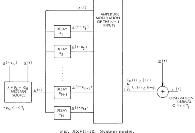
Let us now discuss the equations which describe the system of interest (see
AMPLITUDE MODULATION OF THE N+ 1
DELAY
1
INPUTS
al I
DELAY x(t-a22
x(- N) u(t) w(t) Co (t) x(t) + N x= Fx + G ( x(t-aN-1I
C (t) x (t-ai) r() MESSAGE (t) DELAY + SOURCEN-OBSERVATION INTERVAL -a N < t <n Av x ( t - N O < t < TfFig. XXVII-12. System model.
Fig. XXVII-12).
by a linear state
dx(t)
dt =
F(t)
We assume that the dynamics of the message process are determined
equation
x(t) + G(t) v(t)
over the time interval -aN < t < Tf, where F(t), G(t) are matrices determining the dynamics of the state equation, and v(t) is a white Gaussian source noise with
E[v(t)vT (T)] = Q6(t-T). (2)
In order to completely specify this random process, we need to make some assump-tions about the condiassump-tions of the initial state. We assume that the initial state is a Gaussian random vector with
E[x(-aN)] = (-aN)
We shall now discuss the observation process. We assume that we observe N dif-ferent delayed versions of an amplitude modulation of the state vector in the presence of a white Gaussian observation noise. Our observation is, therefore,
N
r(t)
=
C (t) x(t) +
C (t) x(t-a
i) + w(t),
(5)
i=l
where 0 <t <Tf 0 < a < a2 <... < aN-1 < aN (6) E[w(t)_wT (T)] = R6(t-T). (7)Notice that our observation equation is defined over a different time interval from the state equation. For convenience, let us define
Yi(t) = x(t- a). (8)
Aside from the delay terms that enter, our assumptions do not differ from the usual ones made in state-variable estimation procedures.
3. Derivation of the MAP Estimation Equations
It can be shown that the problem of maximizing the a posteriori density is equivalent to minimizing the following quadratic functional:
J(v(t),x(-aN)) = x(- aN)-(-aN) 1P-aN)
+ f
Lx~t
1 dt - N (9)T
+
a
v(t) -1 dt (9)N
Q
Subject to the constraint of the state equation (1) and the delay operations specified by Eq. 6 (xA = xTAx).
Let us first consider the state-equation constraint. We can introduce this by using a Lagrangian multiplier. This is done by adding to the quadratic functional the term
(XXVII. DETECTION AND ESTIMATION THEORY)
T fT
dx(t)
L =
p (t)
dt
-
F(t) x(t) -G(t) v(t)) dt.
(10)
aN
It will be useful to integrate the first term of the integrand by parts. Doing this, we
have
Lo =p
(Tf) x(Tf) - pT(-aN)x(-a
N )Tf
d
(t) x(t) + pT(t) F(t) x(t) + pT (t) G(t) v(t) dt.
(11)
dt
N
When we incorporate the constraints imposed by the delays, we encounter much
more difficulty.
In order to impose the constraints, we must find a differential
equa-tion that the delay operaequa-tion satisfies.
As we would expect from the infinite-state
requirement imposed by the delay operation, we cannot find a finite-dimensional
ordi-nary differential equation.
It is easy to show, however that the delay operation
satis-fies the partial differential equation
_ i(t, T) a_ i(t, T)
+
=0,
(12)
at
aT
where
_i(t, 0) = x(t).
We show this by noting that the general solution to Eq. 12 is
i (t,
7)
= f (t-T).
(13)
Imposing the boundary condition at T = 0 yields
.i(t, 0) =f.(t)
=
x(t).
(14)
-1 -1
We see that we now have
4.(t,
a.) = f.(t-a.) = x(t-a ) =y.(t).
(15)As a result, we are able to impose the constraint of each delay term by using a
Lagrangian multiplier that is a function of two variables, that is, we want to add to the
quadratic functional terms of the form
1 0
Tf
ai F t T(t
'T)
(t'T)
L.
=,
+
dtdT,
(16)
(17)
We again want to perform some integrations by parts.L.
=
f
(
(t, a.).(t, a.)
(t, 0)
(t, 0)
dt
- -i i 1a
i T T + _ (Tf, T) i(Tf, T)-.L (0, T) .(0 ,T) dT - 0Tfa i
a
(t,)
at
This yields T+
.((t,
T) IT ---.) (t,T)dtdr.
When we add the Lagrangian multiplier constraints Lo, L1, ... LN imposed by the state
equation and the delay terms to the quadratic functional described by Eq. 9, we have
J(v(t),x(-aN))
=
x(-aN)-P(-aN) -(-aN T r(t) - C (t) x(t)T
aN
i=1
C.(t) y.(t)
1 -1v(t) 1-1 dt +p
Tf)(Tf)
x(T) - p T(T ) x(To)
T fdp (tM T T-dt
x(t) + p (t) F(t) x(t) + p (t)
aNG(t) v(t)
I + i=li
T(t , ai )Yi(t)-T (t , 0)x(t)(T
,
T)x(T
-T)--4
(0,7)x(-)
/
T
Tf aI
(t
T
0 0
t
T
+ i(t.T , 7) dtd . IT7We now are in a position to minimize the quadratic functional by applying variational
techniques.
We proceed by perturbing v(t) and x(-aN) from their optimal estimates,
that is,
QPR No. 84
(t, T) = x(t-T). _ 1 (18)(19)
R-1 247(XXVII. DETECTION AND ESTIMATION THEORY)
x(-aN) = x(-aN) + E6x(-aN) v(t) = v(t) + E6(t).
The response of the state equation to the perturbed input is
x(t)
= ^(t) + Ex(t),where 6x(t) satisfies the differential equation d62(t) dt= F(t) 8x(t) + G(t) 6v(t). dt
(20)
(21) (22) (23)The variation by the quadratic functional which results from these perturbations is given
by
J(v(t),x(-aN))
=
J(v(t),x(-aN)) +
TE
P
P- 1
(-a) 5x(-aN)(-aN) &x(-aN
x(
N)x(aN)T
[x(-aN)-x(-aN)]
r(t) -
C (t)
Ox(t)
N
C-
C(
y.(t)
i= tR- 1 Co(t) 8x(t)
N + C (t) 8y (t)j= 1
Tf ^T
+
v(t)
aN
T fN
N i=l dp (t)dt
Q-16(t)
dt + p (T )
6x(Tf)
- p (TT
0) 6x(-aN)(
T x5x(t) + p (t) F(t) 6x(t) + p (t) G(t)
6v(t)f dtSTf
0i=l [
dT]
T a.00
T
a1j (t, T)at
+
T A T6c.(t,
7) 87 1 dtdT} + 0(E ). (24)T
f
+0
N
+ i i= 1 T(t, a)6y (t)- L
T
(t,
0) 5x()
d
T
T
(TfV)6x(T T-)- 1 . (0,T)5x( T)We now want to combine the various variations into common factors. We have
J(y(t),x(-aN)) = J(v(t),x(-aN)) +
E
1x( aN)-5(-aN)]
x-
N )IT
P 1(-aN)-pT(-aN)) bx(-aN)N
- C (t) x(t) -
Cit)
j= 1
N
p T(t) F(t)
-i=1
t,
S (t,0)
Tf
(
0
-
r(t)
-
Co(t)
x(t)-07T
yi(t)
6X(t)
dt-
-p~t
p t) F(t)
dp
T(t)
dt
N
j=
1
N
(t) F(t)-
k
j=i+l
N
j=1
KTf
T + . (t7)
t,+
OT/6c.(t
T) dtdT . (25)We shall now make a series of arguments to cause the
Evariation of the functional
to vanish. We shall require that the Lagrangian multiplier functions satisfy some
equa-tions so that the coefficients of some of the variaequa-tions vanish.
First we require the delay constraints to have the functional form
_i(t, T) = .(t-T) (26) 1
QPR No. 84
-
rt)
R- C (t)
0+Yff
+ ,~T0
dp T(t)
dt
Tf aNi+
i= 1 + (t, a (t) dt 1 i-C (t) j(t
R -1 C.(t)1(t)0
+
N1 N-1i=l
N
j=1
6x(t) dt
T (0, -t)-J3
a.
06x(t) d
Op.. (t, 7)
(
at
)
YO\
at T -1 T ^ ((V(t) Q p (t)G(t))5v(t)) dtLj(Tf,
T)
6x(Tf-_)
249(XXVII. DETECTION AND ESTIMATION THEORY)
so that the last term in the equation vanishes identically ([ii is the adjoint function for the delay equation). Furthermore, we require that
(t- ) = 0 (27) a. < T < T (28) 1 f and, for 0 <t <Tf, (t-a) = CT(t) R r(t) - C (t) _(t)-1 j= Cj(t)
(t
.
(29)This completes our restrictions of the Lagrangian multipliers for the delay
straints. Notice that the restrictions may be made independently of all the other
con-straints, including the state-equation constraint.
Now we shall impose some restrictions on the Lagrangian multiplier for the
state-equation constraint.
First we impose the restriction, 0 < t < Tf,
dt F C (t)
R(t)yj(t)
(t) - Co(t(t) )j=1
N
j=1
3
(30)
Finally, we impose restrictions for the time before the observation interval.
region, for -al < t < 0, we require
N
dp(t)
T
- - F (t ) p(t) -
4o(t),
dt
1
0j=1
and, for -ai+
<
t<
a.,
i = 12,...
N- 1,
N
dp(t) Ndt
-F T(t) p(t) -
L
(t)
dt 1 .j=i+ 1
As a
have
Within this(31)
(32)result, we have defined p(t) over the entire interval of the process.
Therefore we
J(v(t), x(-aN)) = J(V(t),~(-aN))
+ c
(^(-aN))-_(-aN) TP1(-aN)
T-aN)
5x(-aN)
+
f ((t)
Q
1-p (t(t)G(t)) 6v(t) + 0(e2) . (33)Because of the optimality of v(t) and x(-aN), we have
p(-aN)
=P
1(-aN)(((-aN))-_(-aN))
(34)
-1^ T
Q
v(t) = G (t) p(t). (35)Equation 34 imposes an initial boundary condition, and Eq. 35 relates the terms v(t) and
p(t).
By using Eq. 35, our state equation becomes
dx(t)
dt
=
F(t)
x(t)+ G(t) QG(t) p(t).
(36)
We shall now summarize our equations determining the MAP interval estimate of the
process x(t).
For convenience, we shall define
a =0
y
(t) = x(t).For -aN <t <Tf, we have
d^(t)
dt
T
F(t) x(t) + G(t) QG (t) p(t).
By using the definitions stated above, we may write Eqs. 33 and 35 in the same manner.
for -ai+
< t <-a. these equations become
N
dp(t)
T
dt
-F (t) p(t)-
o
(t ),
dt 0
j=i+l
where i may assume the values
i = 0, 1, ...
N-1.
For 0 < t < Tf, we have
dp(t)
o1
dt
=
-F(t) p(t) - Co(t) R
- 1(r(t)
-N
j=0
N
j=
1
The functions i. are defined to be, for 0 <
T< ai,
Soi(T -T) = 0, -o f
and for 0 < t < Tf,
(t-a) = CT(t) R-~o-
1
j
1
r(t)
-j=0
QPR No. 84
Cj(t) yj(t
251Cj(t) y(t
.
(XXVII. DETECTION AND ESTIMATION THEORY)