Corrélation stratigraphique stochastique de puits

HAL Id: tel-01750420

https://hal.univ-lorraine.fr/tel-01750420

HAL is a multi-disciplinary open access archive for the deposit and dissemination of sci-entific research documents, whether they are pub-lished or not. The documents may come from teaching and research institutions in France or

L’archive ouverte pluridisciplinaire HAL, est destinée au dépôt et à la diffusion de documents scientifiques de niveau recherche, publiés ou non, émanant des établissements d’enseignement et de recherche français ou étrangers, des laboratoires

Corrélation stratigraphique stochastique de puits

Florent Lallier

To cite this version:

Florent Lallier. Corrélation stratigraphique stochastique de puits. Sciences de la Terre. Université de Lorraine, 2012. Français. �NNT : 2012LORR0414�. �tel-01750420�

AVERTISSEMENT

Ce document est le fruit d'un long travail approuvé par le jury de

soutenance et mis à disposition de l'ensemble de la

communauté universitaire élargie.

Il est soumis à la propriété intellectuelle de l'auteur. Ceci

implique une obligation de citation et de référencement lors de

l’utilisation de ce document.

D'autre part, toute contrefaçon, plagiat, reproduction illicite

encourt une poursuite pénale.

Contact : ddoc-theses-contact@univ-lorraine.fr

LIENS

Code de la Propriété Intellectuelle. articles L 122. 4

Code de la Propriété Intellectuelle. articles L 335.2- L 335.10

http://www.cfcopies.com/V2/leg/leg_droi.php

´

ecole doctorale RP2E

TH`

ESE

pr´esent´ee et soutenue publiquement le 14 Novembre 2012 pour l’obtention du grade de

Docteur de l’Universit´

e de Lorraine

Sp´ecialit´e G´eosciences

par

Florent LALLIER

Corr´

elation stratigraphique

stochastique de puits

Directeur de th`ese : <sub>Jean Borgomano</sub> Co-directeur de th`ese : _{Guillaume Caumon}

Sophie Viseur

Composition du jury :

Rapporteurs : Jef Caers

Philippe Joseph

Examinateur : Emmanuelle Vennin

Remerciements

Voici donc venu l’heure d’´ecrire les derni`eres lignes de cette th`ese.

Je tiens tout d’abord `a remercier Emmanuelle Venin d’avoir accept´e pr´esider mon jury de th`ese, que Jeff Caers et Philippe Joseph d’avoir accept´e rapporter mes travaux de th`ese, ainsi que Julien Charreau d’avoir accept´e de participer `a ce jury. Je vous remercie ´egalement et tout particuli`erement pour la discussion qui a suivi mon exposer.

Mes remerciements vont ensuite `a mes directeurs de these. Un grand merci `a Guillaume Caumon qui m’a guide dans le monde de la G´eomod´elisation depuis mes d´ebuts. Merci Chef pour ta confiance et pour m’avoir laiss´e autant de libert´e. Un grand merci ´egalement `

a Sophie Viseur, ton enthousiasme et tes conseilles avis´es m’ont ´et´e d’une grande aide. Un grand merci enfin `a Jean Borgomano. Merci d’avoir accept´e de diriger ma th`ese et merci fait d´ecouvrir la g´eologie des syst`emes carbonat´es. Je remercie Julien Charreau pour m’avoir ouvert les portes de la magn´etostratigraphie. Merci de m’avoir fait d´ecouvrir une face pour moi inconnue de la g´eologie. Merci ´egalement a Christophe Antoine pour tout ce tu as apport´e `a ce projet magneto’ mais aussi pour tout ce que tu as apport´e `a cette th`ese en g´en´eral.

Je remercie aussi tous les membres de l’´equipe de recherche Gocad, les CPRGiens et les Marseillais. Fatima, merci pour tout, pour les petits et les grands coups de main. Merci Pierre et encore une fois non, ce n’ai pas moi qui ai fait planter les ordinateurs. Merci Pauline (CD) pour toute les discussions, les rires et les blagues et le soutient au quotidien. Et merci `a Christine, parce que tu as ´et´e ma premi`ere prof d’informatique et parce que j’aimais te croiser pour un caf´e.

Merci aux co-thesards, compagnons de luttes gocadiennes, les anciens et les nouveaux. MarcO – le plus ancien de tous et mon premier chef ; Thomas et Vincent - les co-bureaux et champions de volleyball ; Jeanne – merci pour tes multiples relectures jusqu’`a l’ultime, 30 minutes avant la soutenance ; Francois – ou Fifid’Or, et avec toi Julie et Arthur ; Romain et Jeremy ; Charline – un ´enorme merci pour tout ce que tu as apport´e `a cette th`ese, Gauthier – je ne comprends toujours pas comment ils font pour prendre un bain avec simplement un mini morceau de tissus blanc ; C´ecile – merci de m’avoir h´eberge et d’avoir support´e mon ignorance de la suisse. Merci `a Nico Cherpeau, co-these et co-loc, compagnon de route tropico depuis le d´ebut, merci pour les coups de main et les `a-cˆot´es. Et puis merci `a Pauline (DR), merci pour tes conseils, les innombrables relectures, ton soutient, et surtout merci d’avoir ´et´e la du d´ebut `a la fin.

Je finirai en remerciant ce qui ´etait l`a au tout d´ebut, ma sœur Pauline, mes Pa-rents, ma et mon nourrisse et tous les autres. Merci, de m’avoir soutenu, d’avoir ´et´e la et de m’avoir laiss´e aller ou bon me semblais.

Table des mati`

eres

Introduction 1

1 Stratigraphie s´equentielle et m´ethodes stochastiques de corr´elation

stra-tigraphique de puits 5

1.1 Motivation and related works . . . 10

1.1.1 Need for a stochastic approach . . . 10

1.1.2 Automatic well correlation, a review . . . 11

1.2 Proposed framework for sequence stratigraphic correlation . . . 15

1.2.1 Key points of the proposed approach . . . 15

1.2.2 DTW for multi-well correlation . . . 15

1.2.3 Integrating geological constraints . . . 17

1.2.4 Uncertainty management . . . 18

1.3 Application to outcrop data of the Beauset Bassin . . . 18

1.3.1 Geological settings and material . . . 18

1.3.2 Stochastic well correlation . . . 20

2 Corr´elation d’unit´es diag´en´etiques `a partir de donn´ees diagraphiques : des incertitudes sur l’interpr´etation d’une sismique haute r´esolution `a leur impact sur les ´ecoulements de fluides 29 2.1 Introduction . . . 32

2.2 Stratigraphic correlation method . . . 35

2.2.1 Correlation rules . . . 35

2.2.2 Evaluation of the value of a correlation between two units . . . 35

2.2.3 Automatic stratigraphic correlation between two wells . . . 37

2.3 Results and discussions . . . 38

2.3.1 Stratigraphic correlation models . . . 38

2.3.2 Property modelling . . . 39

2.3.3 Seismic response to alternative stratigraphic models . . . 40

2.3.4 Implications on fluid flow modelling . . . 42

2.4 Conclusions . . . 43

3 Utilisation de l’imagerie sismique comme contrainte dans le processus de corr´elation stochastique de puits 45 3.1 Introduction . . . 47

3.2 One Algorithm for Stratigraphic Correlation . . . 48

3.3 Correlation Rule R1ased on Well Log . . . 50

3.4 Correlation Rules from Seismic Data . . . 50

3.4.2 Correlation Rule R3ased on a Stratigraphic Seismic Attribute . . . . 52

3.5 Application . . . 56

3.6 Conclusion . . . 57

4 Magn´etostratigraphie automatique : M´ethode de gestion des incertitudes sur l’ˆage des roches et sur les taux d’accumulation de s´ediments 59 4.1 Le champ magn´etique terrestre et son enregistrement dans les roches . . . . 60

4.1.1 Description et origine du champ magn´etique terrestre . . . 60

4.1.2 L’alimentation r´emanante d´etritique . . . 61

4.1.3 Reconstruction de l’histoire des inversions du champ magn´etique ter-restre : l’´echelle de r´ef´erence . . . 62

4.2 Magn´etostratigraphie : principes et m´ethodes . . . 65

4.2.1 Construction d’une colonne magn´etostratigraphique . . . 65

4.2.2 Corr´elation `a l’´echelle de r´ef´erence . . . 66

4.3 Gestion des ambiguit´es lors de corr´elations magn´etostratigraphiques . . . . 66

4.3.1 Computer method for magnetostratigraphic correlation . . . 71

4.3.2 Application to recent magnetostratigraphic analyses in Central Asia 81 4.3.3 Certainty and uncertainty on sediments age and accumulation rates 86 4.4 Etudes compl´´ ementaires : analyse de la fonction coˆut . . . 90

4.5 Perspectives . . . 92

Conclusions g´en´erales 93

Table des figures

1.1 Etapes de la mod´´ elisation d’un r´eservoir . . . 9

1.2 Syst`emes carbonat´e et incertitude angulaire . . . 12

1.3 Composantes de l’algorithm DTW . . . 14

1.4 Principe de la corr´elation stratigraphique stochastique . . . 16

1.5 Algorithme DTW ´etendu `a plusieurs dimensions . . . 17

1.6 Probl´ematiques des boucles dans le chemin de corr´elation . . . 18

1.7 Algorithme DTW it´eratif . . . 19

1.8 G´eographie et pal´eog´eographie du Beausset . . . 20

1.9 Charte stratigraphique de l’intervalle ´etudi´e . . . 21

1.10 Relation trigonom´etrique entre ´epaisseur de s´ediment et profondeur de d´epˆot 23 1.11 Calcul du coˆut d’un horizon `a partir d’une pal´eog´eographie th´eorique . . . . 24

1.12 Construction d’une repr´esentation th´eorique de la pal´eog´eographie du Beausset 25 1.13 Mod`eles stratigraphiques de la marge carbonat´ee Sud Proven¸cal . . . 27

2.1 Stratigraphy of the Malampya buildup . . . 33

2.2 Evaluation of similarity between log responses of two units . . . 35

2.3 Sections of diagenetic units model . . . 38

2.4 MA-1 to MA-2 cross-section of acoustic impedance models . . . 39

2.5 MA-1 to MA-2 cross-section of synthetic seismic . . . 40

2.6 NRMS computed along the MA-1 to MA-2 section . . . 41

2.7 Permeability models and oil saturation at different time steps . . . 44

3.1 The successive steps of a proposed worflow . . . 48

3.2 The DTW algorithm . . . 49

3.3 Building an implicit 3D stratigraphic model . . . 52

3.4 Computation of the thinning attribute . . . 53

3.5 Thinning attribute on Vail’s system tract . . . 54

3.6 Building study zone to compute the cost between two units . . . 54

3.7 The three cases for the calculation of a correlation cost from the thinning attribute . . . 55

3.8 Reference correlation . . . 57

3.9 Stratigraphic well correlations between the wells w1 and w2 . . . 58

4.1 Composantes du champ magn´etique terrestre . . . 61

4.2 L’aimantation r´emanente d´etritique . . . 62

4.3 L´egende sur la page suivante . . . 64

4.3 Construction de la GPTS . . . 65

4.5 Contraintes sp´ecifiques aux applications magn´etostratigraphiques . . . 76

4.6 Caption on next page. . . 80

4.6 Test sur un jeu de donn´ees synth´etique . . . 81

4.7 Caption on next page. . . 83

4.7 R´esultat de datation sur le coupe Xishuigou . . . 84

4.8 Caption on next page. . . 85

4.8 R´esultat de corr´elation pour la coupe Yaha . . . 86

4.9 Densit´e de probabilit´e de l’´epaisseur d’un chron . . . 88

4.10 Coˆut en fonction du rang de la corr´elation . . . 91

Liste des tableaux

Introduction

La repr´esentation du sous-sol, qu’elle soit num´erique ou analogique, g´eom´etrique ou physique, est construite dans deux buts : comprendre et pr´edire. Lors de l’´etude d’un objet g´eologique, plusieurs repr´esentations peuvent en ˆetre propos´ees en fonction de la probl´ematique envisag´ee. Plusieurs exemples peuvent ˆetre donn´es :

– L’´etude d’un r´eservoir (p´etrolier ou aquif`ere) a pour buts de pr´edire : (i) la capa-cit´e contenue ; et (ii) la circulation des fluides (dans une perspective de production ou de diffusion de contaminant). `A chaque fois, mod´eliser le r´eservoir consistera `a d´eterminer la r´epartition des h´et´erog´en´eit´es lithologiques ou p´etrophysiques.

– Pour comprendre l’histoire du remplissage d’un bassin s´edimentaire, le g´eologue s’in-t´eressera `a construire un mod`ele repr´esentant les isochrones et ainsi sont ´evolution temporelle. Le remplissage d’un bassin s´edimentaire ´etant contrˆol´e par des facteurs tectoniques, environnementaux et climatiques, sa repr´esentation temporelle permet de pr´edire les pal´eoclimats, reliefs ou paysages.

– Dans une ´etude g´eotechnique, on s’int´eresse `a repr´esenter les caract´eristiques m´ e-caniques du sous-sol. Cette repr´esentation sert de base pour pr´edire la r´eponse du sous-sol lors de la construction d’un ouvrage d’art.

Depuis les ann´ees 1990 et sous l’impulsion du d´eveloppement d’une nouvelle g´en´eration de logiciels d´edi´es aux probl´ematiques g´eologiques, la repr´esentation du sous-sol passe par la construction de mod`eles tridimensionnels associant g´eom´etrie des objets g´eologiques et propri´et´es physiques. Les donn´ees et informations disponibles pour la construction d’un g´eomod`ele sont de natures diverses. On peut ainsi distinguer :

– les donn´ees d’affleurements ou issues de forages carott´es. Il s’agit de donn´ees directes permettant une description lithologique `a fine ´echelle. Les caract´eristiques physiques des roches ´etudi´ees peuvent y ˆetre mesur´ees pr´ecis´ement en laboratoire sur des ´ echan-tillons (appel´es plugs) pr´elev´es. Ces donn´ees, localis´ees et peu nombreuses, n’offrent qu’une vision limit´ee de la g´eom´etrie tridimensionnelle des objets ´etudi´es ;

– Les donn´ees de puits : diagraphie et imagerie. Ces donn´ees permettent, apr`es inter-pr´etation, d’acc´eder `a la description des types de roches rencontr´ees et `a certaines de leurs caract´eristiques. Comme pour les affleurements, les donn´ees de puits sont localis´ees et souvent peu nombreuses ;

– Les donn´ees g´eophysiques telles que l’imagerie sismique, 2D ou 3D, les donn´ees issues de mesures gravim´etriques ou ´electromagn´etiques. Ces donn´ees sont globales mais de faible r´esolution et peuvent amener `a des interpr´etations contradictoires Bond et al. [2007] ;

– Les concepts g´eologiques, tel que les concepts de stratigraphie s´equentielle, conf´erant un cadre th´eorique `a l’interpr´etation des donn´ees observables ;

Construire un g´eomod`ele, c’est mettre en coh´erence l’ensemble des donn´ees et connais-sances disponibles. Les donn´ees disponibles sont cependant locales, de r´esolution inf´erieure au mod`ele souhait´e, ou ambig¨ues. De plus, les objets g´eologiques ´etudi´es ont ´et´e mis en place par des processus nombreux, interd´ependants et souvent mal connus voire inconnus. Il en r´esulte que, `a partir de mˆemes donn´ees et de mˆemes informations, plusieurs repr´ e-sentations du sous-sol ´etudi´e peuvent ˆetre propos´ees. C’est dans ce contexte qu’intervient le concept d’incertitude en g´eomod´elisation, c’est-`a-dire lorsque le manque d’informations ou le manque de qualit´e de celles-ci ne permet pas d’en construire un seul et unique mod`ele.

Les m´ethodes g´eostatistiques telles que les simulations gaussiennes s´equentielles (SGS), les simulations s´equentielles d’indicatrices (SIS), les simulations par gaussiennes tronqu´ees [Deutsch et al., 1998] et les m´ethodes bas´ees objet [Deutsch and Wang, 1996, Viseur, 2004], entre autres, sont des exemples de m´ethodologies permettant de g´erer les incertitudes en g´eomod´elisation. Dans le cas de la mod´elisation de propri´et´es p´etrophysiques, les simula-tions permettent de g´en´erer un grand nombre de r´ealisations (en th´eorie, un nombre infini) en tenant compte des donn´ees disponibles : valeur de propri´et´es au puits, donn´ees g´ eophy-siques (dans le cas de co-simulations), histogrammes et variogrammes. Dans cet exemple, plusieurs sources d’incertitudes peuvent ˆetre identifi´ees :

– le manque de donn´ees : seuls les puits, souvent peu nombreux, fournissent des valeurs pr´ecises de propri´et´es ;

– Le manque de r´esolution des donn´ees secondaires dans le cas de co-simulations ; – La qualit´e des mesures, que ce soit pour les donn´ees g´eophysiques ou pour les mesures

aux puits ;

– Le variogramme utilis´e. En effet, dans le cas d’´etudes de r´eservoir p´etrolier, le vario-gramme est mod´elis´e `a partir de peu de points de donn´ees. Ainsi, pour ˆetre construit, le mod`ele de variogramme utilis´e n´ecessite une interpr´etation de la part du g´eologue, int´egrant entre autres des connaissances issues d’analogues ;

– L’espace dans lequel sont calcul´ees les distances. En effet, dans le cas d’h´et´erog´en´eit´es li´ees aux faci`es de d´epˆot par exemple, la distance entre des points correspond `a la distance stratigraphique d´efinie par la g´eom´etrie et la topologie des horizons et failles interpr´et´es par le mod´elisateur. Cette g´eom´etrie, construite `a partir des donn´ees cit´ees pr´ec´edemment, est elle-mˆeme sujette `a incertitudes.

Probl´

ematique de la mod´

elisation stratigraphique

Les travaux pr´esent´es dans ce m´emoire s’inscrivent dans le contexte d´efini par les deux points pr´ec´edent, c’est-`a-dire les incertitudes li´ees `a la subjectivit´e des interpr´etations pro-pos´ees par le g´eologue, et celles li´ees `a la g´eom´etrie et `a la topologie des fronti`eres des diff´erent objets g´eologiques ´etudi´es. Dans le cas de roches s´edimentaires, ces fronti`eres sont issues de deux types de processus : les processus s´edimentaires contrˆolent la g´eom´etrie (en partie) et la topologie des horizons stratigraphique, les processus tectoniques contrˆolent la

Introduction

g´eom´etrie et la topologie des r´eseaux de failles et des horizons stratigraphiques (directe-ment lorsqu’on s’int´eresse aux plissements et indirectement via le contrˆole structural des processus s´edimentaires).

Nous nous int´eressons dans ce m´emoire `a la topologie des horizons stratigraphiques. Celle-ci est d´efinie par la corr´elation stratigraphique d’unit´es identifi´ees au niveau des puits. Cette ´etape de corr´elation stratigraphique est l’une des premi`eres du processus de construc-tion d’un g´eomod`ele dans les formations s´edimentaires. Elle consiste `a associer les diff´erentes unit´es stratigraphiques identifi´ees le long des puits et affleurements disponibles. Ces unit´es stratigraphiques sont d´efinies de sorte qu’elles repr´esentent chacune un ensemble coh´erent refl´etant par exemple : une s´equence de d´epˆots (cas de la stratigraphie s´equentielle), une mˆeme lithologie (cas de la lithostratigraphie), un mˆeme ensemble de caract´eristiques p´ e-trophysiques ou encore une mˆeme pal´eo-orientation du champ magn´etique terrestre (cas de la magn´etostratigraphie). Dans le processus de corr´elation stratigraphique, le g´eologue est confront´e `a deux choix distincts :

1. Quelle r`egle utiliser pour d´efinir les unit´es stratigraphiques ? Ce choix est dict´e par les facteurs contrˆolant les caract´eristiques du sous-sol que l’on cherche `a repr´esenter. Par exemple, dans le cas de l’´etude d’un r´eservoir p´etrolier, le g´eomod`ele est utilis´e pour repr´esenter les h´et´erog´en´eit´es p´etrophysiques des roches. Les h´et´erog´en´eit´es p´ e-trophysiques peuvent ˆetre contrˆol´ees par exemple par (i) les faci`es de d´epˆots – les principes de stratigraphie s´equentielle pourront alors ˆetre utilis´es pour d´efinir les uni-t´es stratigraphiques `a corr´eler ; ou (ii) par la diagen`ese ayant affect´e les roches apr`es leur d´epˆot – une approche lithostratigraphique pourra alors ˆetre choisie.

2. Comment sont associ´ees, entre les puits, les diff´erentes unit´es stratigraphiques iden-tifi´ees ? Il s’agit de la probl´ematique de corr´elation stratigraphique, abord´ee dans ce m´emoire. Cette ´etape cl´e d´efinit la topologie et en partie la g´eom´etrie des horizons stratigraphiques correspondant aux fronti`eres des objets g´eologiques ´etudi´es. Selon le sch´ema de construction d’un g´eomod`ele le plus r´epandu, la construction des corr´ ela-tions stratigraphiques est confi´ee `a un g´eologue stratigraphe qui, manuellement et de fa¸con d´eterministe, d´efinit les associations entre unit´es stratigraphiques. Consid´erant les remarques qualitatives et quantitatives faites pr´ec´edemment sur les informations et connaissances disponibles pour r´esoudre le probl`eme de corr´elation stratigraphique, nous sugg´erons dans ce m´emoire de le traiter de fa¸con stochastique afin d’´ echantillon-ner les incertitudes associ´ees.

`

A partir d’un algorithme g´en´eral de corr´elation stochastique d´eriv´e de l’algorithme de d´eformation temporelle dynamique (plus connu sous le nom anglais : Dynamic Time Warping algorithm), diff´erentes r`egles de corr´elation stratigraphique sont propos´ees afin de traiter plusieurs cas naturels. Ce m´emoire s’organise autour de quatre articles ayant chacun pour cadre d’´etude un syst`eme naturel diff´erent. Chacun de ces articles d´ecrit : (i) l’algorithme g´en´eral utilis´e pour g´en´erer de fa¸con stochastique les corr´elations stratigraphiques ; (ii) les adaptations de cet algorithme afin de prendre en compte les

particularit´es de l’application ; (iii) les r`egles de corr´elation stratigraphique utilis´ees.

Le premier chapitre sert d’introduction `a la probl´ematique de corr´elation stra-tigraphique. Une premi`ere pr´esentation de la m´ethode stochastique de corr´elation stratigraphique est propos´ee. `A partir de l’´etude des s´equences de d´epˆots de la plateforme carbonat´ee Sud-Proven¸cale d’ˆage Cr´etac´e sup´erieur, une m´ethode multi-puits et stochas-tique de corr´elation de s´equences stratigraphiques est pr´esent´ee. Deux r`egles de corr´elation des horizons bordant les s´equences de d´epˆots sont introduites. Celles-ci s’appuient sur les caract´eristiques g´eom´etriques th´eoriques de l’environnement de d´epˆot : ´evolution coh´erente des pal´eo-angles et des ´epaisseurs de s´ediments d´epos´es ; repr´esentation th´eorique de l’espace de d´epˆot.

Le second chapitre s’int´eresse `a l’impact des incertitudes li´ees aux corr´elations stratigraphiques sur la mod´elisation statique et dynamique du r´eservoir carbonat´e de Malampaya (situ´e au Nord-Ouest de l’ˆıle de Palawan aux Philippines). Pour ce faire, deux r`egles de corr´elation bas´ees sur la r´eponse diagraphique des unit´es stratigraphiques (unit´es diag´en´etiques dans ce cas) et sur le type lithologique sont propos´ees. Plusieurs mod`eles de r´eservoir, construits `a partir de diff´erents mod`eles de corr´elation g´en´er´es de fa¸con stochastique, sont construits et analys´es en fonction de leur comportement dynamique et de leur r´eponse sismique.

Une m´ethodologie permettant de prendre en compte les donn´ees issues de l’imagerie sismique est propos´ee dans le chapitre trois. Cette m´ethodologie, coupl´ee `a une r`egle de corr´elation bas´ee sur les tendances pr´esentes au niveau des enregistrements diagraphiques, est appliqu´ee `a la corr´elation stratigraphique de d´epˆots fluviaux delta¨ıques de la Mer du Nord.

Enfin, une m´ethode de gestion et de visualisation des incertitudes dans le cas des cor-r´elations magn´etostratigraphiques est propos´ee en chapitre quatre. Nous proposons alors de calculer les n meilleures corr´elations entre une colonne magn´etostratigraphique issue d’´etudes de terrain et une colonne de r´ef´erence, permettant ainsi de dater les s´ediments ´etudi´es et d’estimer les pal´eo-taux d’accumulation de s´ediments et les incertitudes asso-ci´ees.

Chapitre 1

Stratigraphie s´

equentielle et

m´

ethodes stochastiques de

corr´

elation stratigraphique de

puits

Sommaire

1.1 Motivation and related works . . . . 10

1.1.1 Need for a stochastic approach . . . 10

1.1.2 Automatic well correlation, a review . . . 11

1.2 Proposed framework for sequence stratigraphic correlation . . . . 15

1.2.1 Key points of the proposed approach . . . 15

1.2.2 DTW for multi-well correlation . . . 15

1.2.3 Integrating geological constraints . . . 17

1.2.4 Uncertainty management . . . 18

1.3 Application to outcrop data of the Beauset Bassin . . . . 18

1.3.1 Geological settings and material . . . 18

1.3.2 Stochastic well correlation . . . 20

La construction de corr´elations stratigraphiques, dans le cadre d’une ´etude de r´ eser-voir ou de bassin, permet notamment de subdiviser le volume ´etudi´e en sous-ensembles o`u les variables ´etudi´ees (faci`es ou propri´et´es p´etrophysiques) r´epondent aux crit`eres de sta-tionnarit´es n´ecessaires `a la plupart des m´ethodes g´eostatistiques utilis´ees pour simuler ces variables. Dans ce contexte, l’utilisation des concepts d´efinis par la stratigraphie s´ equen-tielle pour construire ces corr´elations apporte une aide pr´ecieuse.

Ceci est d’autant plus vrai lors de l’´etude de r´eservoirs ou bassins carbonat´es o`u la r´ eparti-tion spatiale des s´ediments r´esulte de processus s´edimentaires nombreux et interd´ependants. Ainsi, compte tenu de la complexit´e de l’architecture stratigraphique r´esultante, la construc-tion de corr´elations stratigraphiques entre les diff´erents puits ou affleurements disponibles est sujette `a de nombreuses incertitudes. Nous proposons ici de prendre en compte ces incertitudes en utilisant une m´ethode stochastique pour g´en´erer ces corr´elations stratigra-phiques. Cette m´ethode est bas´ee sur l’algorithme de d´eformation temporel (ou Dynamic Time Warping, DTW), qui a d´ej`a ´et´e utilis´e qvec succ`es la corr´elation de s´eries ordonn´ees

en bio-informatique et en reconnaissance de la parole. Trois versions de cet algorithme sont propos´ees dans ce chapitre : (i) une version stochastique permettant de g´en´erer plusieurs mod`eles probables de corr´elation ; (ii) une version multi-puits utilisant un tableau `a n di-mensions afin construire des mod`eles de corr´elations stochastiques entre n puits ; (iii) une version it´erative permettant corr´eler stochastiquement n puits. Cette derni`ere m´ethode re-quiert moins de m´emoire vive et permet ainsi de corr´eler un grand nombre de puits. De plus, une approche hi´erarchique est propos´ee, les unit´es stratigraphiques d’ordre inf´erieur sont corr´el´ees en premier et les corr´elations r´esultantes sont utilis´ees pour contraindre la corr´elation des unit´es d’ordre sup´erieur. Dans ce chapitre, l’algorithme DTW est utilis´e afin de construire des mod`eles de corr´elation respectant les r`egles de stratigraphie s´equentielle. Deux r`egles de corr´elation sont propos´ees pour assurer la coh´erence des pal´eo-angles et celle entre les faci`es d´ecrits aux puits et la pal´eo-g´eographie suppos´ee du milieu de s´edimentaire ´etudi´e.

La m´ethode propos´ee est appliqu´ee dans ce chapitre `a la corr´elation d’unit´es stratigra-phiques identifi´ees le long des affleurements de la marge carbonat´ee sud-proven¸cale d’ˆage Cr´etac´e Sup´erieur.

Uncertainty assessment in stratigraphic

well correlation : a new stochastic method

for carbonate reservoir

Article to be submitted to the AAPG Bulletin

Florent Lallier , Guillaume Caumon , Jean

Borgomano , Sophie Viseur, Jean-Jacques Royer

Abstract

An application of well correlation is to subdivide a reservoir into stationary intervals to support geostatistical modelling of static reservoir properties. In this scope, sequence stratigraphic well correlation appears to be an efficient technique, especially in carbonate sedimentary systems resulting from numerous and interdependent genetic processes. Ho-wever, due to the complexity of sedimentary layers, well correlation is a hazardous process which is subject to many uncertainties. In this work, we propose to account for these un-certainties by generating several possible realizations of well correlations. The method is based on the Dynamic Time Warping (DTW) algorithm, whose efficiency has already been demonstrated in speech recognition and bio-informatics. Three derivative versions of the DTW algorithm are introduced : a stochastic one for correlating two wells (2D DTW) ; a multi-well one, which accounts for the 3D organization of stratigraphic architectures by analysing all input wells at once. Due to computation time and memory requirements, this version is limited to the correlation of up to ten wells. To address this issue, an iterative multi-2D DTW based on well correlation propagation is proposed. In addition, the propo-sed algorithms integrate stratigraphic order of well markers to perform the well correlation hierarchically (low frequency stratigraphic events are correlated first, and then are used to constrain the correlation of higher-order events). To perform stratigraphic correlation with DTW algorithms, one has to compute the likelihood of each possible horizon. Because of the high significance of chronostratigraphy in siliciclastic and carbonate reservoir modeling, the presented likelihood computation is based on paleo-angles consistency and facies and sedimentary profile coherency. This stochastic correlation algorithm and the influence of stratigraphic correlation uncertainties on static reservoir modelling are demonstrated on outcrop data of the Cretaceous southern Provence Basin (Provence, S-E France).

Introduction

Well data represent 1-D information about subsurface heterogeneities. Because wells are often placed in potentally high-pay areas the set of available wells, reduced to the mini-mum due to drilling costs, is thus often sparsely spread over the study area and corresponds to an incomplete and possibly biased sampling of the subsurface objects and heterogenei-ties. As defined by Doveton [1994a] manual methods for well correlation are slow, highly labor-intensive, sometimes inconsistent and are often subject to uncertainty. Moreover, as demonstrated by Bond et al. [2007] for seismic interpretation, knowledge introduced to fill the lack of data may introduce bias depending on interpreter’s background. As a conse-quence, well correlation is an under-constrained problem, leading to several possible results (sets of correlation).

Stratigraphic well correlation aims at linking correlative units between available wells [Doveton, 1994a] and thus helps defining the 3D structure of the studied reservoir or basin. In practice, a 3D geometrical model of the studied reservoir or basin is built from well correlations which define stratigraphic architecture and horizons and faults picked on a

γ1 γ0 γ0 γ1 1: Stratigraphic correlation 4: Facies simulation 6: Flow simulation 3: Geostatistical study 2: 3D geometric modeling

5: Petrophysical property simulation

Figure 1.1 – Simple reservoir modeling workflow. Stratigraphic correlations constrain the geometry of the grid that will support geostatistical analysis and facies and rock property modeling.

seismic survey (Fig.1.1). This geometrical model is used to control the construction of a grid on which two types of coordinates are defined [Dubrule and Damsleth, 2001, Deutsch, 2002] : the absolute coordinates (x, y, z) and the stratigraphic coordinates (u, v, w) which are use to perform geostatistical analysis and property modelling. Uncertainties on well correlation, which affect stratigraphic coordinates result on uncertainties on petrophysical property modelling, definition of flow units and thus may have a high impact on hydrocarbon resource assessment and production prediction.

Uncertainties on a 3D reservoir model can be achieved by generating several possible models which then serve for OHIP computations or reservoir simulations [Samson et al., 1996] [Charles et al., 2001]. For example, to handle structural uncertainties, Lecour et al. [2001] propose to perturb the geometry of the reference model, Holden et al. [2003], Cher-peau et al. [2010] stochastically generate fault networks. However, for stratigraphic well correlations, in our knowledge, no stochastic method hence perturb both the model’s topo-logy and the geometry taking uncertainties into account has been proposed.

Our objective is to introduce a numerical method to build stochastically stratigraphic well correlations. Algorithm frequently used to build stratigraphic correlation automatically are reviewed in section 1.1.2. In this study, the Dynamic Time Warping algorithm [Myers and Rabiner, 1981] is used. Derivative versions of this algorithm to perform stochastic, hierarchical and multi well correlation are presented in section 1.2.

Well correlation may be achieved in different ways, and using different well descriptors (markers, facies, wireline logs, etc.). Several authors propose computer aided approaches to perform correlations between wells on the basis of logs [Zoraster, 2004] or lithostratigraphic

description [Griffiths and Bakke, 1990, Olea, 2004]. In the case of few wells spread over the area of study, the relevance of sequence stratigraphic well correlation as a basis for 3D static reservoir modelling has been demonstrated by Ainsworth et al. [1999], Ainsworth [2005] for siliciclastic settings and by Borgomano et al. [2008] for carbonate environment. Therefore, in this paper, we consider well data which correspond to sequence stratigraphic intervals identified from the depositional facies. The method proposed in this paper allows to stochastically correlate stratigraphic sequences according to sedimentological rules.

After reviewing numerical methods for well correlation problem (section 1.1), specific algorithms for multi-well stochastic stratigraphic well correlation are presented in section 1.2. Correlation rules and application of the stochastic approach to Cretaceous outcrops of the southern Provence Basin (South-East France) is presented in section 1.3.

1.1

Motivation and related works

1.1.1 Need for a stochastic approach

Combinatorial point of view. Considering two wells with respectively n and m iden-tified stratigraphic markers and assuming that top and bottom markers of each well are correlated together, the number (Dn,m) of possible correlations between these two wells is

given by the Delanoy number defined as :

Dn,m = Dn,m−1+ 2 n−1 ∑ i=0 Di,m−1 D1,1= D1,n= D1,m= 1 (1.1)

This equation can be extended in d dimensions, i.e. to enumerate the number of correlations between d wells with respectively ni markers per well as follows :

Dn1,··· ,nd = Dn1−1,··· ,nd + Dn1,n2−1,··· ,nd + · · · Dn1,··· ,nd−1

+ D_{n1−1,n2−1,··· ,nd} + · · · + D_{n1−1,n2,··· ,nd−1}

· · ·

+ D_{n1−1,··· ,nd−1}

(1.2)

Two simple examples can highlight the practical meaning of these equations :

– Per equations 1.1, the number of possible correlations between two wells, with only ten markers on each well,is equal to D10,10= 1, 462, 563 possible correlations.

– Stratigraphic correlation of twelve wells with respectively seven markers on each, Eq.(1.2) leads to 1080possible correlation models, which is equivalent to the number of atoms in the universe.

1.1 Motivation and related works

Among this huge set of possible well correlations, only some of them are geologically sound and it is very difficult to explore and to appreciate manually the different plausible solutions of well correlation. The use of a stochastic method able to account for geological constraints to generate well correlation models would hence appear to be an appreciable tool to sample the possibly large set of plausible correlations.

A geologic point of view. In spite of sedimentological rules used to perform well cor-relation, interpreters often face ambiguities between many different plausible correlations. As shown by Borgomano et al. [2008] and Koehrer et al. [2011], when available wells do not allow to relate the subsurface heterogeneities several sets of well correlation may match sedimentological rules.

In the case of low average-angle carbonate ramp or platform, performing sequence stratigra-phic well correlation consists in correlating meter thick sequences between kilometers-apart wells. Many stratigraphic sequences observed along borehole are beyond seismic resolution and have to be correlated on the basis of stratigraphic rules. However, due to the thickness of sequences to correlate, distances separating wells, and uncertainty on angle of paleo-sedimentary profiles, well correlation becomes uncertain (Fig.1.2). It follows that, given a range of possible average paleo angles, alternative well correlation models can be built.

1.1.2 Automatic well correlation, a review

Many authors, following the work of Sackin et al. [1965], proposed numerical methods to automatically perform well correlations. Such automatic methods are essential to handle uncertainties. A review of numerical methods used to perform well correlation is proposed by Doveton [1994a]. Three mains algorithms are described in the literature :

– The Dynamic Time Warping algorithm which is derived from bio-informatic and speech recognition [Levenshteiti, 1966, Myers and Rabiner, 1981] is used by Smith and Waterman [1980] to build the lithostratigraphic correlation of two outcrops located in Kansas.

– Neural networks are used by Bursik and Rogova [2006] to perform the lithostratigra-phic correlation of volcano deposits.

– Expert systems are used by Olea [1994, 2004] for the correlation and interpretation of wireline logs.

This work focuses on the Dynamic Time Warping algorithm that is based on a repre-sentation of the correlation between two wells in a 2D table. Considering two wells W1 and

W2 with respectively n and m stratigraphic markers, the stratigraphic correlation between

these two wells is represented as a path in a cost table D (Fig.1.3A and B) built up with a series of points and transitions (respectively correlation of markers and intervals). The geological consistency of each possible correlation between markers and between units and each possible unconformity is evaluated independently thank to the computation of a cost. These costs are stored in the table as follows :

Well spacing: 10km

Sequence a verage thic kness: 25m B C D α = 0.05° ? ? α = 0.15°

Shelf carbonate Slope Carbonate

Ambiguity

in correlation between two sequences Ambiguity in correlation between n sequences 0 10 20 30 40 50 60 70 80 0 0,05 0,1 0,15 0,2 0,25 0,3 0,35 0,4 0,45 V e rti ca l e rr o r a lo n g w e ll (m ) Angular error α (°) Well spacing: 10km 8km 6km 4km 2km A

Figure 1.2 – In the case of carbonate ramp characterized by low average angle carbonate ramp, uncertainty α on average angle impacts well correlation. (A) Impact of errors in average paleo-angles on error in position of the horizon along the well for different well spacings. (B) Given a synthetic model of carbonate ramp (B), (C) An error of 0.5◦ in the evaluation of the average paleo-angle results on ambiguities on the correlation between two units 10m thick between (C). When the angular error reaches 0.15◦, the ambiguity is between three units (D).

1.1 Motivation and related works

– A point at cell (i, j) corresponds to the correlation between the marker i of the first well W1 and the marker j of the second well W2 with a cost c(i, j).

– An oblique transition corresponds to a correlation between two intervals (the interval

{i; i − 1} of W1 and the interval{j; j − 1} of W2) with a cost noted tj,ji,i−1−1 in Eq.(1.3).

– A vertical transition between cells (i, j) and (i− 1, j) means that the interval {i; i − 1} of W1 end in an unconformity between units j; j− 1 and j + 1, j of W2. This

unconformity is associated to a cost noted tj,j_i,i−1. An horizontal transition corresponds to an unconformity with a cost tj,j_i,i−1.

The total score of a path is calculated as the sum of all the costs c and t contained in this path. The minimum cost path from the bottom left cell (bottom correlation line [1, 1]) to the top right cell (top correlation line [n, m]) corresponds to the optimal correlation between W1 and W2. The minimum cost correlation path through the table is obtained by

computing iteratively the minimum cost path from the bottom right cell to the cell (i, j) thanks to :

D (i, j) = c (i, j) + min

   tj,j_i,i−1−1+ D (i− 1, j − 1) tj,j_i,i−1+ D (i− 1, j) tj,j_i,i−1+ D (i, j− 1)    (1.3)

Once the entire DTW cost table has been filled, the correlation path is searched starting at cell [n; m] as shown in figure 1.3. The next cell is the one with the minimun cost, between the three adjacent cells (on the left, bottom and diagonally to the bottom-left). The search then continues from this cell, using the same rule, until the bottom left is reached. This construction method makes the correlation path unidirectional, ensuring there is no overlap. The correlation is thus consistent.

As shown by Bashore et al. [1994], the choice of the correlation strategy has a great impact on static and dynamic reservoir modelling. In DTW the obtained stratigraphic archi-tecture depends on correlation rules use to evaluate the consistency of correlation between units or markers. Many studies on automatic well correlation based on the DTW algorithm focused on the development of these correlation rules [Smith and Waterman, 1980, Howell, 1983, Waterman and Raymond Jr., 1987, Fang et al., 1992a, Collins and Doveton, 1993]. Fang et al. [1992a] perform the correlation of stratigraphic units on the basis of wireline log attributes, Griffiths and Bakke [1990] define numerical lithologies based on gamma-ray, density, neutron and velocity log responses and perform correlation between wells using gene typing rules including the possibility of lateral facies substitution. Waterman and Raymond Jr. [1987] define rules on the basis of lithostratigraphic type, grain size and units thickness and Collins and Doveton [1993] compute the likelihood of the correlation between two units thanks to a vertical Markov transition analysis along well. These methods are mainly based on a lithostratigraphic description of facies. As a result, the probability of the correlation of two units is the same for wells 10km appart than for wells 1km apart.

Cost table D n i W 1 W₂ 1 1 j m m 1 i 1 n j W₁ W₂ W₂ W₁ k k-1 l-1 l C D E A B Unacceptable correla on Unacceptable correla on

Figure 1.3 – 2D DTW for stratigraphic correlations. A) Stratigraphic correlation between two wells W1 and W2 containing respectively n and m markers. The thick line is the

correlation between the ith marker of W1 and the jth marker of W2 (correlation line [i; j])

which is is assumed to be known a priori. B) DTW cost table D displaying the minimum cost correlation path. Due to the hard correlation [i; j] (thick point in the table), two parts of the cost table are removed, these positions corresponding to impossible correlations.

C, D and E : elements to evaluate to perform stratigraphic correlation within the DTW

algorithm ; correlation between units{k; k − 1} of W1 and {l; l − 1} of W2, units {k; k − 1}

1.2 Proposed framework for sequence stratigraphic correlation

1.2

Proposed framework for sequence stratigraphic

correla-tion

1.2.1 Key points of the proposed approach

Considering well data as a ranked list of stratigraphic markers, stochastic well correla-tion may be seen as a method that stochastically links well markers of different wells one with another. Geologists use sedimentological rules and regional knowledge to obtain geolo-gically sound correlations. Depending on these rules and constraints, a correlation between two well markers would appear more plausible than other ones. Similarly, in our method the correlation process first evaluates the likelihood of all possible elementary correlation lines between well markers (figure 1.4) and then, randomly chooses a set of marker correlations according to this likelihood. Therefore, several sets of correlation can emerge from the same correlation rules, which translates the imperfection of these rules while precluding unlikely correlations. Each outcome of the method, associating all markers of all considering wells, is termed a realization because it samples correlation uncertainty. The algorithm proposed in this paper relies on this key idea in the Dynamic Time Warping framework.

Unlike previous studies which assign constant value to the correlation cost between stratigraphic units (t term of the Eq.(1.3)) [Smith and Waterman, 1980, Fang et al., 1992a] or compute it as a function of units thickness [Waterman and Raymond Jr., 1987], our well correlation technique is only based on the evaluation of stratigraphic horizon consistency (term c in Eq.(1.3)). Moreover, our method considers sequence stratigraphic units identified along wells. Resulting well correlation thus defines the sequence stratigraphic architecture of the studied area.

To perform sequence stratigraphic well correlation, the first step is to formulate the sedimentological rules into a mathematical expression that estimates the cost of correlating two given markers (Section 1.3.2). The second point is the modification of the DTW algo-rithm to perform well correlation stochastically. Moreover the well correlation algoalgo-rithm is built in order to take into account for hard constraints such as regional correlation lines and to use stratigraphic hierarchy to constrain well correlation. The well correlation algorithm should also perform multi well correlation, by taking into account the 3D structure of the studied horizons.

1.2.2 DTW for multi-well correlation

Most of the time, the well correlation problem is not limited to a simple correlation between two wells but needs to consider all available wells at once. On the basis of the Dynamic Time Warping algorithm, two strategies are proposed.

Multi-dimentional DTW

When more than two series must be correlated, Brown [1997] proposes to increase the dimension of the DTW table. The procedure is simple : a 2D cost table is used for the

INITIAL DATA EVALUATION OF THE LIKELIHOOD OF ALL POSSIBLE HORIZONS

ST OCHASTIC GENERA TION OF POSSIBLE WELL CORRELA TION GENERATED CORRELATION MODELS

Figure 1.4 – Stochastic sequence stratigraphic correlations workflow

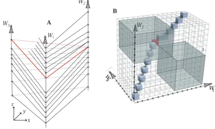
correlation of two wells, a 3D table for three wells and so on. In this representation, each cell of the table corresponds to the association of one marker of each well. This approach offers the possibility to correlate all available wells at once. Hence, it can take into account the 3D geometry of the deposition environment for each correlation likelihood computation. However, the time and memory complexity O(nm), with n the number of markers per well and m the number of wells, is prohibitive, and limits its applicability to a dozen of wells. Moreover, with a simple implementation of this algorithm, the correlation of 12 wells with 10 stratigraphic markers on each requires 4 Gigabytes of RAM to store the cost table. In bioinformatic applications it was proposed to reduce the computational time of the procedure by assuming that the minimum score path is close to the main diagonal of the cost table (see [Brown, 1997] for an application to stratigraphic correlation and Fullen [1997] for a review of optimization methods). In our case, this optimization is possible only in a globally conformable stratigraphic setting.

Multi 2D DTW

A way to decrease the computational time and the memory requirement of the multi well correlation is to correlate all wells two at a time by considering each pair indepen-dently. To achieve this, a correlation path is built to define the pairs of wells that are to be correlated. In addition, loops are prohibited to avoid conflicting results (Fig. 1.6). In practice, the correlation path is computed by extracting the minimum spanning tree bet-ween studied wells. This strategy has the asset of the time performance but can only be done for simple elementary correlation cost and to not allow to account for global trends to perform stratigraphic correlation. Indeed, when correlating wells i and j correlations of

i and j with all other available wells contains information that are not contained in i and j only. Therefore, we have developed an iterative DTW (Fig. 1.7). First all pairs of wells

of the correlation path are correlated. So that, for each pair p of the correlation path, all previously correlated pairs (i from 1 to p− 1) are known and used to compute the current

1.2 Proposed framework for sequence stratigraphic correlation W3 W1 W2 x y z A W₂ A B W 1 1 W 3

Figure 1.5 – DTW based on a 3D table A) 3D representation of the wells correlation. B) 3D DTW Cost Table and correlation path for the correlation of the three wells.

correlation. Then, the computed correlation of a randomly drawn pair of the path is deleted and rebuilt taking into account all other correlations. This ensures that every correlation is generated knowing the whole 3D stratigraphic structure.

1.2.3 Integrating geological constraints

Three levels of constraints can be used to perform well correlation using the DTW algorithm.

– A correlation line interpreted by a geologist can be an input constraint. This constraint is represented as a fixed point in the DTW table (see thick line and point on Fig.1.3A and B). Due to the correlation path construction and to the input cor-relation line [i, j] in Fig.1.3B), some positions become unacceptable in the table. As a result, the correlation problem is divided in two and two DTW tables are used : one to compute the correlation path from [1, 1] to [i, j], and another one to compute the correlation path from [i, j] to [n, m] (Fig. 1.3B). The correlation path is thus constrained to pass through this point, and the overall performance of the algorithm is significantly improved.

– Stratigraphic sequences identified along the well bore can be ordered using strati-graphic sequence hierarchy [Vail et al., 1977] or fractal nature [Schlager, 2004, Neal, 2009, Schlager, 2009]. Lowest stratigraphic orders markers (sensu Vail et al. [1977]) are correlated first to constrain higher order markers correlation. To introduce such a capability, first stratigraphic order markers are correlated thanks to the DTW algo-rithm, and resulting correlation lines are used as input correlation line in the DTW for the correlation of higher stratigraphic orders markers.

– Correlation rules used to compute cost within the DTW algorithm are a third level of constraint because they drive the way correlation likelihoods of n markers are

1 2 3 1 1 2 2 3 3

Figure 1.6 – Exemple of inconsistent well correlation (thick line) generated using three classical DTW. This inconcistency is due to the loop (1 2 3) described by the correlation path

evaluated.

1.2.4 Uncertainty management

As discussed in section 1.1, well correlation is a complex problem and Waterman and Raymond Jr. [1987] and Griffiths and Bakke [1990] propose to generate several realizations of correlations by modifying cost computation rules, leading to generate a model per geo-logical scenario. Our method may not only use several senarios, bur also generates various models from one single scenario using a stochastic function to fill the DTW Cost Table. From the current location (i, j) in the DTW cost table, we propose to randomly draw the next location by replacing Eq.(1.3) by : D (i, j) = f (a, b, c, d) where p is a random value drawn from a uniform distribution U [0, 1], and a (respectively b and c) is the probabi-lity of making an oblique (respectively vertical or horizontal) transition in the DTW table (Eq.1.4). f (a, b, c, p) =      1/a if p∈[0,_a+b+ca [ 1/b if p∈[ a a+b+c, a+b a+b+c [ 1/c if p∈[ a+b a+b+c, 1 ]      with a = 1/(c (i, j) + tj,j−1_i,i−1 + D (i− 1, j − 1) ) b = 1/(c (i, j) + tj,j_i,i−1+ D (i− 1, j) )

c = 1/(c (i, j) + tj,j_i,i−1+ D (i, j− 1) ) (1.4)

1.3

Application to outcrop data of the Beauset Bassin

1.3.1 Geological settings and material

The Beausset basin is located in Basse-Provence, southeastern France (Fig. 1.8 a). The studied area corresponds to a carbonate platform, aged Cenomanian-Middle Turo-nian, which developed on the southern part of the “Durance swell” [Philip, 1974]. These

1.3 Application to outcrop data of the Beauset Bassin 4 3 1 2 5 6 7 1 7 4 3 2 5 6 4 3 1 2 5 6 4 3 1 2 5 6 7 7 Step 1 Step 2 Step 6

While neded

Remove one two wells correlation

Rebuilding the two wells correlation knowing the other correlations

map

A : Correlation Path B: Building of a first draft correlation set trough the path

C: Iterative deletion and rebuilding of the correlation of pairs

Figure 1.7 – Iterative DTW algorithm. From a correlation path (A), a first correlation draft between wells is built (B) using a sequential 2D DTW. At each step of (B), the previously built correlations are known and used as a constraint. Then, to ensure the 3D consistency of the correlation, a random correlation between two wells is removed and rebuilt given all other correlations (C). In the deterministic DTW, this process is performed until sum of the pair-wise scores alonf the spanning tree is no longer modified by the iterative loop. In the case of stochastic DTW the number of loops to perform is defined empirically.

Exposed Area Basinal Facies

Heterozoane Carbonates

Terrigenous Input Extent of the Coniacian carbonate platform.

6km

N

a b

Figure 1.8 – a) Geographic and paleogeographic settings of the study area. After Philip [1993]. b) Location of studied outcrops

deposits display terrigenous inputs from a crystalline Hercynian basement corresponding to the southeastern limit of the basin (Fig. 1.8). Multiple outcrops have been described in this area [Philip, 1974, 1993, Philip and Gari, 2005, Gari, 2007]. These almost continuous outcrops from platform to basin deposits allowed previous authors to build well constrained geometrical model and sequence stratigraphic correlations.

Outcrop data

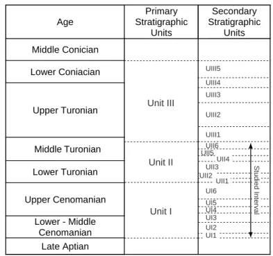
The studied outcrops are aged lower Cenomanian to middle Turonian (Fig.1.9). Nine outcrops sections covering the entire studied interval, are used in this study (Fig. 1.8). The studied interval is subdivided in two primary stratigraphic units : U.I and U.II [Gari, 2007]. U.I, aged Cenomanian, correspond to the transgressive part of a second order, sensu Vail et al. [1991], transgressive regressive cycle ending mid Turonian [Philip, 1998]. This unit is divided into six secondary stratigraphic units (U.I 1 to U.I 6), bounded by conspicuous surfaces or abrupt facies changes corresponding to 3rdand 4thorder cycles. The U.II primary stratigraphic unit, aged lower to mid Turonian, is the regressive part of the 2nd order cycle started in U.I. This unit is also divided into six secondary stratigraphic units (U.II 1 to U.II 6). Following the outcrop description and study proposed by Gari [2007], eight facies have been distinguished according to the depositional depth range, bioclastic content and deposition style (Table 1.1).

1.3.2 Stochastic well correlation

Correlation rules

Two methods for the evaluation of the consistency of a horizon are used : (i) a paleoangle based rule which compares markers by pairs and (ii) a depositional facies based rule which uses all available markers of the considered horizon at once.

1.3 Application to outcrop data of the Beauset Bassin Age Primary Stratigraphic Units Secondary Stratigraphic Units Middle Conician Lower Coniacian Upper Turonian Middle Turonian Lower Turonian Upper Cenomanian Lower - Middle Cenomanian Late Aptian Unit III Unit I Unit II UIII5 UIII4 UIII3 UIII1 UIII2 UII5 UII6 UII3 UII2 UII1 UI2 UI3 UI4 UI5 UI6 UI1 UII4 Studied Interval

Figure 1.9 – Chronostratigraphic and sequence stratigraphic subdivision of the Creta-ceous southern Provence Basin. The studied interval is composed of twelve fourth order hemicycles.

1.3.2.1 Paleoangle consistency

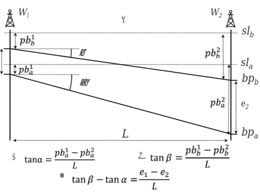
To check the consistency of a stratigraphic correlation of a carbonate ramp, Borgomano et al. [2008] introduce trigonometric relationships between average paleo-angles (α and β) of two considered horizons and sediment thicknesses (e1 and e2 respectively on wells 1 and

2) according to (Fig. 1.10) :

(tan(β)− tan(α)) = (e1− e2

L ) (1.5)

This formalism is adapted to compute a cost of stratigraphic correlation between two mar-kers using a prior defined correlation line, extracted for instance from seismic data. From the paleobathymetry at markers a priori correlated (pb1_a and pb2_a), the paleobathymetry of the studied markers (pb1_b and pb2_b) and the sediment thicknesses (e1 and e2), we compute

the cost C as the degree of violation of the theoretical formula 1.5 when computing the terms using paleo-bathymetric data as follows :

C = (pb1_a− pb2_a)− (pb1_b − pb2_b)− (e1− e2) (1.6)

This method is valid in the case of a regular accommodation increase between the two correlated wells. In the case of a differential subsidence, a rotation angle has to be added to Eq.(1.6) [Borgomano et al., 2008].

Facies Minimun bathymetry of deposition

Maximum bathymetry of deposition

value uncertainty value uncertainty

F0 : Charophyte Limestones -50 0 0 0 F1 : Micritic Limestones 0 -5 1 5 F2 : Bioclastic Limestones with Rudists 5 3 10 5 F3 : Bioclastic Limestones with Rudists and Corals

7 4 15 5

F4 : Bioclastic Limestones with fragment of Rudists and Corals

15 5 50 10

F5 : Argilous Limestones 50 25 100 25

F6 : Marl and Marly Limes-tones

125 25 175 –

F7 : Brecia, Lobe, Grainflow and Debris flow

40 10 175 –

Table 1.1 – Facies described by their possible depositional bathymetry. This description is used to build the depositional space presented in figure 1.12 and to interpolate bathymetry along wells. Modified after Gari [2007].

This correlation rule relies on a well log describing the bathymetry of deposition. The method used to compute this curve in this study has been proposed by Kedzierski et al. [2008] : it uses interpolation method Mallet [2002] constrained by facies depositional depths described in table 1.1.

1.3.2.2 Sedimentary profile consistency

Boundaries of stratigraphic sequences identified on wells could be considered as time si-gnificant [Catuneanu et al., 1998]. Consequently, markers bounding stratigraphic sequences could be taken as a sparse sampling of the geography (i.e. sedimentary profile) at the time of deposition. Evaluating the likelihood of a correlation line then boils down to checking whether this sampling is consistent with the paleogeography.

In practice, the cost of the considered horizon, i.e. a set of correlated stratigraphic markers (one per well) is computed as follow :

1. A map representing the theoretical paleogeography is built. The probability of depo-sition of each facies is defined on the map.

2. The considered correlation horizon is set back into the depositional space using for instance a map restoration method. Each considered marker is thus defined by its facies and its deposition space coordinates.

1.3 Application to outcrop data of the Beauset Bassin

W

W

sl

sl

bp

bp

L

α

β

e

Figure 1.10 – Trigonometric relationships on a carbonate ramp system (from Borgomano et al. [2008]). These relations are used to check the consistency of a marker correlation : using measurement in A and relations B and C, the equality D is true if the correlation is good. Notations : pb is the paleobathymetry at the current marker ; sl the sea level ; L the well spacing ; bp the base profile ; e1, e2 the decompacted sediment thicknesses ; α, β the

F0 F7 Depositional Facies

basin-ward land-ward

a: Studied horizon in the geological space

x y

x

y z

b: Markers transfered into depositionnal coordinates

c: Best fitting position between makers and probability of deposition is searched in the depositional space according to facies deposition probability .

F0 deposition probability map

F1 F5 F7

Figure 1.11 – Likelihood computation using theoretical sedimentary profile. a) Studied horizon and markers displaying depositional facies in the geological space. b) Studied mar-kers transferred into the depositional space coordinate system. c) Likelihood computation : the best location of the set of markers is searched in the depositional space (see Fig.1.12) according to the deposition probability of each facies. The likelihood is computed as the sum of these probabilities.

1.3 Application to outcrop data of the Beauset Bassin 0 50 150 250 0 0 100 200 1 0 probability 1 depth F0 F1 F2 F3 F4 F5 F6/F7 F5 F6 F1 F3 a b c

Figure 1.12 – Construction of a map describing the palaeography using equations of slope geometry [Adams and Schlager, 2000] and membership function. a) sedimentary profile built from shoreline, regular increase of bathymetry in the shelf with an angle = 0.5◦, a shelfbreak at 40 meter depth and a slope described using exponential equation. b) Mem-bership functions for the description of the location of facies using bathymetry (see Table 1.1). c) Examples of possible location of deposition for facies 1, 3, 5 and 6.

3. The best fitting configuration of this set of markers in the theoretical deposition space is searched so that it maximizes the sum of facies probabilities at markers. Due to the low degree of roughness of the considered map, we use the gradient descent method. 4. The cost is computed as the inverse of the facies probabilities sum (Fig.1.11).

The theoretical deposition space may be built using seismic attributes computed on derived from 3D high resolution seismic volumes [Baaske et al., 2007]. When seismic ima-ging is poor, we propose to build it using membership functions [Mallet, 2002] describing the bathymetry of deposition of each facies (Fig. 1.12). Membership functions, coupled to a sedimentary profile geometry built from 2D seismic lines or using equations proposed by Adams and Schlager [2000], allow to build probabilistic pictures of the depositional environment. However, in most depositional settings, facies type is not controlled by the bathymetry only. Membership functions allow addressing this by defining facies deposition location as a probability range.

1.3.2.3 Constraints

The top and bottom horizons of the studied interval (U.I 1 and U.II 6 in Fig.1.9) are input as known correlations to constraint the stochastic well correlation process. These horizons are also used as a priori known correlations to compute correlation costs based on paleoangles (section 1.3.2.1).

1.3.2.4 Results and discussions

Geometrical model and grid building Four alternative models are built (Fig.1.13 B, C, D, and E) : a reference model built from the deterministic correlation proposed by Gari [2007] (Fig.1.13 B) and three models built from the stochastically generated correlations (see Section 1.2.4) using the iterative DTW algorithm (see Section 1.2.2).

The geometry of these four models is constrained by the geometry of the top and the bottom horizon of the studied interval (U.I 1 and U.II 6 in Fig.1.9)). These two horizons have been built by Gari [2007] using intersections with the topography and dip and strike measurements on field. Internal horizons corresponding to well correlations, are build so that they respect well markers and the thickness variations of units defined by surfaces are smoothed [Mallet, 2002]. A conformable stratigraphic grid is then built for the reference model and the stochastic ones.

Facies distribution analysis Vertical proportions of facies are calculated for each stratigraphic model (Fig.1.13). This vertical proportion of facies can be analyzed in terms of reservoir facies distribution, assuming that facies F0 to F4 are potentially reservoir and facies F5 to F7 are flow barriers. Because outcrops located on the North side of the basin display a continuous record of reservoir facies, any model built from the stochastic correlations results in compartmentalization of the reservoir. However, the four models

1.3 Application to outcrop data of the Beauset Bassin Z N E

A

B

C

D

E

F0

F1

F2

F3

F7

F6

F5

F4

Figure 1.13 – Set of possible stratigraphic models of the Cretaceous southern Provence basin. A : 3D deterministic stratigraphic model of the basin (from Gari [2007]). The black lines indicate the location of the studied outcrops ; the shaded surface the location of the cross-sections presented in B to E. B : Stratigraphic correlation model proposed by Gari [2007] and associated vertical proportions of facies. The dash lines are the projected loca-₂₇

presented in figure 1.13 (representing a small subset of the possible stratigraphic correlation models) show two alternative views of the distribution of reservoir rocks : in the models B and D, reservoir facies are concentrated into two main groups whereas in models C and E, reservoir facies are divided into several units (6 in the model C and 5 in the model D) separated by flow barriers. Alternative stratigraphic correlation models thus result in different reservoir compartmentalization scenarios. Additional information coming from well production, such as well PLT could be used to select stratigraphic correlation models. Alternative stratigraphic correlation models may also interpretations of the sedimentary and tectonic history of the stlead to different udied area. For instance, Gari [2007] interprets the unit U.I 6 as a prism constituted of marls whose deposition is due to a tectonic tilting. In relation with this tectonic activity, the production of carbonate is stopped on the platform, suggesting a confinement and hypoxic event. In contrast, such a hypoxic event could not be interpreted if the model E is considered, because the equivalent prism is correlated to platform deposits.‘

Conclusions

The presented algorithms offer the possibility to generate several possible stratigraphic correlations of a study area. These automatic methods offer reliable computation of corre-lation parameters (paleoangle, distance). Several stratigraphic correcorre-lations can be quickly generated, which was challenging when manually performing the correlations. Moreover, the generated correlation sets can be constrained by prior knowledge such as correlation lines extracted from seismic data or/and hypothetical base profile geometry. Several geolo-gical senarios may be tested in agreement with prior geologeolo-gical knowledge.

Stochastic stratigraphic correlation, combined with geostatistical facies simulation, is a better way to handle uncertainties on reservoir and basin modeling than multiple facies si-mulation on a unique grid. Indeed, it allows propagating the correlation uncertainties down to facies and flow simulations.

Chapitre 2

Corr´

elation d’unit´

es diag´

en´

etiques

`

a partir de donn´

ees diagraphiques :

des incertitudes sur

l’interpr´

etation d’une sismique

haute r´

esolution `

a leur impact sur

les ´

ecoulements de fluides

Sommaire

2.1 Introduction . . . . 32 2.2 Stratigraphic correlation method . . . . 35

2.2.1 Correlation rules . . . 35 2.2.2 Evaluation of the value of a correlation between two units . . . 35 2.2.3 Automatic stratigraphic correlation between two wells . . . 37

2.3 Results and discussions . . . . 38

2.3.1 Stratigraphic correlation models . . . 38 2.3.2 Property modelling . . . 39 2.3.3 Seismic response to alternative stratigraphic models . . . 40 2.3.4 Implications on fluid flow modelling . . . 42

2.4 Conclusions . . . . 43

Lors de la construction d’un mod`ele de r´eservoir, les corr´elations stratigraphiques per-mettent de construire une trame pour la mod´elisation tridimensionnelle des propri´et´es p´ e-trophysiques. Dans le cas du r´eservoir `a gaz Malampaya, la distribution de ces propri´et´es r´esulte de la diag´en`ese de roches carbonat´ees. Mod´eliser un tel r´eservoir n´ecessite de : (1) identifier le long des puits les diff´erentes unit´es diag´en´etiques constitutives du r´eservoir, ces unit´es ´etant des ensembles coh´erents de transformations diag´en´etiques affectant les roches ; (2) corr´eler spatialement ces unit´es diag´en´etiques, ce qui permet de d´eterminer la r´epartition spatiale des diff´erentes unites diag´en´etiques. Dans ce chapitre, une m´ethode de corr´elation d’unites diag´en´etiques est propos´ee. Elle est bas´ee sur l’algorithme DTW pr´esent´e dans le