Computational neutronics analysis of TRIGA reactors during power pulsing

COMPUTATIONAL NEUTRONICS ANALYSIS OF TRIGA REACTORS DURING POWER PULSING

By Malcolm Bean

SUBMITTED TO THE DEPARTMENT OF NUCLEAR SCIENCE AND ENGINEERING

IN PARTIAL FULFILLMENT OF THE REQUIREMENT FOR THE DEGREE OF

BACHELOR OF SCIENCE IN NUCLEAR SCIENCE AND ENGINEERING AT THE

MASSACHUSETTS INSTITUTE OF TECHNOLOGY

MAY 2011

Malcolm Bean. All Rights Reserved

The author hereby grants to MIT permission to reproduce and distribute publicly Paper and electronic copies of this thesis document in whole or in part.

Signature of Author:

Malcolm Bean Department of Nuclear Science and Engineering 23, 2011 Certified

by:---Assistant Pro Lssor

Certified by:

Visiting Associate Professor

Benoit Forget of Nuclear Science and Engineering Thesis Supervisor

Eugene S

fwageraus

Certified by:

-Dennis Whyte

COMPUTATIONAL NEUTRONICS ANALYSIS OF TRIGA REACTORS DURING POWER PULSING

By Malcolm Bean

Submitted to the Department of Nuclear Science and Engineering on May 19, 2011 In Partial Fulfillment of the Requirement for the Degree of

Bachelor of Science in Nuclear Science and Engineering

ABSTRACT

Training, Research, Isotopes, General Atomics (TRIGA) reactors have the unique capability of generating high neutron flux environments with the removal of a transient control rod, creating conditions observed in fast fission reactors. Recently, several TRIGA reactors have had issues with the deformation of fuel rods nearest the transient control rod, where the neutron flux is highest. This is a difficult problem to analyze because the damage is not simply due to rods overheating, but rather the pressurization of hydrogen, from the Uranium Hydride fuel, that has diffused into the spacing between fuel and cladding. Previous neutronic analyses utilized point kinetics; a model which assumes changes in reactivity uniformly affect the reactor's flux, resulting in no relative spatial variation over time. Point kinetics is attractive because of its low computing costs, however the pulse's localization, theoretically, should generate a pronounced flux spike and radial neutron wave, which violates an assumption of point kinetics. The aim of the research is not to explicitly describe the cause of fuel rod deformation, but rather generate time dependent, high-resolution 3-dimensional flux maps. The Purdue Advance Reactor Core Simulator (PARCS) was used to simulate a TRIGA pulse with both nodal and point kinetics. Assuming our nodal kinetics models accurately simulate TRIGA pulses, we find that point kinetics methods are ill suited to simulate TRIGA pulses. By maintaining the steady-state flux profile, point kinetics does not capture the fact that the power peak actually occurs in the center assembly, from which the transient control rod is removed. In our simulations, point kinetics underestimated the normalize power in the central assembly by as much as 46.19%.

Thesis Supervisor: Benoit Forget

Introduction

Training, Research, Isotopes, General Atomics (TRIGA) reactors have the capability to

generate high neutron flux pulses with the removal of a pneumatic transient control rod. The high neutron flux pulse conditions can be used to simulate fast fission and fusion reactors environments, therefore having this capability is critical in testing aspects of new reactor designs, namely radiation damage and radiation effects.

Recently, the Texas A&M TRIGA reactor has had issues with the deformation of fuel rods nearest the pneumatic transient control rod (Remlinger, 2009). During a pulse, the fuel pins nearest the transient control rod experience the highest neutron flux. A previous analysis estimates that component temperatures are significantly higher in that area, but the peak temperatures are below critical values that would cause the observed damage.

With that being said, it is theorized that neutron flux gradients are a larger factor in fuel pin damages, most notably the diffusion and pressurization of hydrogen from the uranium hydride fuel. The rate of hydrogen diffusion is based on the temperature and temperature gradient within the fuel, which in turn are highly correlated to a pin's flux magnitude and profile, respectively.

The past analyses significantly overestimate reactor power during pulsing, with the gap between the simulation and measured data increasing as pulse reactivity worth is increased. Because of this error in the estimated pulse magnitude, the spatial neutron distributions are also in question.

Due to computing limitations, reactor core simulations use homogenized blocks of various sizes as computational units, and then run secondary calculations to recreate the flux profile within the blocks. In the case of the Texas A&M TRIGA reactor analysis point kinetics was used to model neutron flux during a pulse. This method treats the

reactor as a single homogeneous block, where changes in reactivity uniformly affect the reactor's flux, resulting in no relative spatial variation over time.

Point kinetics is attractive because of its low computing costs and accuracy for small perturbations, however the magnitude of TRIGA pulses are significantly larger than those for which point kinetics was derived. The pulse localization, theoretically, should generate a pronounced radial neutron wave, which violates an assumption of point kinetics. The possible errors from point kinetics are then compounded by the application of generic pin flux profiles for fuel rods, which do not account for the steep flux gradients that occur across fuel pin during a pulse.

It should be emphasized that the aim of this report is not to explain the cause of the fuel pin damage. Rather, the report will focus on comparing the three dimensional flux maps produced by point kinetics simulation and the more sophisticated scheme of spatial nodal kinetics. Then by comparing the spatial fluxes produced by the two scheme, give insight into the appropriateness of using point kinetics, or the need to use a finer mesh simulation, when modeling a TRIGA reactor pulse.

Methods

To simulate the Texas A&M TRIGA reactor pulse, Serpent, a Monte Carlo reactor physics burn-up calculation code(Leppanen, 2010), and the Purdue Advanced Reac-tor Core SimulaReac-tor (PARCS), a reacReac-tor core simulaReac-tor(Downar, September 2009), were used in tandem. First, Serpent was used to generate cross sections for fuel and reflector regions, which were then used in PARCS to calculate steady-state and pulse flux dis-trubtions. Further descriptions and details regarding each piece of software and specific utilizations are provided in the following subsections.

PSG2/Serpent

Serpent is a three-dimensional continuous-energy Monte Carlo reactor physics burn-up calculation code, developed at the VTT Technical Research Centre of Finland in 2004. The code specializes in two-dimensional lattice physics calculations for cross section generation. Serpent was used to generate macroscopic cross sectional data for both the point kinetics and nodal kinetics simulations.

Serpent generated energy dependent (via 2 neutron groups) and first-order temper-ature dependent macroscopic neutron transport cross sections from the reactor micro-scopic materials properties and core geometries. Specifically, our simulations utilized the nuclide cross sectional data from the Evaluated Nuclear Data (ENDF/B-VII) and two neutron groups, thermal and fast, were delineated with all neutron energies below 0.625 eV categorized as thermal.

To incorporate temperature dependence, fuel cross sections are calculated at tem-peratures above, below and within the range of temtem-peratures expected during a pulse. Linear interpolations between cross section data are used to produce first-order tem-perature dependent cross sections for core modeling software. Temtem-perature variance in the coolant cross sections based on temperature are not incorporated because a TRIGA pulse is essentially adiabatic.

Explicitly, the Serpent calculated cross sections used in the pulse are the principal cross sections (transport, absorption, v-fission, n-fission), group scattering (both intra and inter-group-scattering), fission neutron spectrum, inverse neutron velocity, delayed neutron fractions and delay neutron precursor decay constants. Temperature depen-dence is only calculated for principal macroscopic cross sections and group scattering.

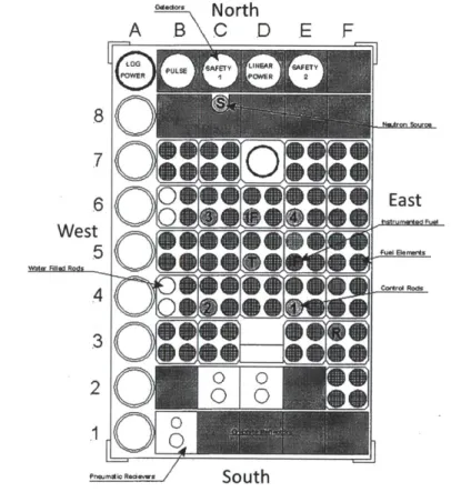
As seen in Figure 1, the basic assembly units of the Texas A&M TRIGA reactor are two by two matrices containing combinations of control rods, fuel rods and water filled

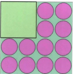
rods. These sets of four pins are the basic neutronic sub-units (homogenized regions) of the simulations. In the lateral plane, the fuel region is surrounded by graphite reflectors to the "north" and "south". In the vertical plane, the fuel rods are capped by graphite reflectors and control rods are followed by the same uranium hydride in fuel rods. The transient control rod is unique in that it is followed by an air void. With the TRIGA reactor being a pool type, it is immersed in a large pool of light water. Figure 2 is a Serpent rendering of a center planar slice of the entire TRIGA core geometry.

adc"

North

A

B\C

D

E

F

7

West

5m

e ft

Figure 1: The layout of the Texas A&M TRIGA reactor as specified in the Nuclear Regulatory Commission's Safety Analysis Report (SAR)

Figure 2: A Serpent rendering of a center planar slice of the TRIGA core geometry. Fuel pins are purple, control rods are beige, water is pink and graphite reflectors are green

Cross Section Generation Details

To generate cross sections for our PARCS model, six reactor sub-unit cross sections were calculated. The sub-units were a fully loaded fuel assembly (C5), a half loaded fuel assembly (B6), water reflector (D7), graphite reflector (E8), an assembly with a control rod (E4) and the transient control rod assembly (D5). The coordinate system listed after each subunit corresponds to an example of that sub-unit's location depicted

Each sub-unit was placed in the top right corner of a two by two box, surrounded by three fully loaded sub-units. Reflective boundary conditions were imposed outside boundary. This was critical for the graphite and water reflector because a source of neutrons is required to generate cross sections. Figure 3 is an illustration of the geometry used to generate cross sections for water reflector. Figure 4 illustrates the geometry used to generate cross sections for an assembly with a control rod. Note that homogenized cross sectional data was taken from the areas outlined in black.

Figure 3: Serpent geometry for calculating the water cross sectional data

Each layout has six branch cases: fuel temperature is set to 373"C, 6234C and 873"C, and at each of those temperatures two branches are generated, with the control rod removed and inserted. In all cases, moderator temperature was set to 23'C. The un-rodded 373 0C fuel temperature branch was used as the reference. From the reference case fuel temperature and control material effect, partial derivates were calculated. Obviously, four of the sub-units (graphite reflector, water reflector, fully loaded fuel

000

Figure 4: Serpent geometry for calculating control rod containing assembly cross sectional data

assembly and half loaded fuel assembly) do not contain a control rod, therefore their control material effect partial derivates are set to zero. This must be done for cross section data file consistency (Downar, December 2009).

To improve cross section data accuracy, the entire reactor core geometry can be modeled with Serpent, and each assembly and section of reflector in the reactor can be treated as a unique sub-unit. This approach was initially attempted, but was abandoned as it seemed to cause convergence issues in the PARCS model. In hindsight it was most likely a faulty parameter in either the PARCS model, or a single cross section data file, that was causing this issue. By only using six sub-units, we could individually test cross section data file. Having each assembly and reflector section of the reactor treated as a unique sub-unit would require checking 119 separate files.

Purdue Advanced Reactor Core Simulator (PARCS)

PARCS has the capability to perform nodal kinetics calculations for transients. For our point kinetics model a use Matlab simulation is used to calculate power and reac-tivity. Steady-state flux profile is assumed throughout pulse. Using the homogenized region cross section data generated by Serpent, PARCS calculates steady state and pulse neuronic conditions. In PARCS the pneumatic removal of center control rod will be simulated as a "control rod perturbation", the equivalent of a control rod ejection in a power generating nuclear reactor.

In the PARCS model the horizontal division of the reactor core matches the Ser-pent model exactly. Each fuel assembly and graphite block is approximately 7.71cm by 7.71cm squared. Axially, the reactor is divided into 14 regions, ten-3.81cm slices representing the uranium-hydride rich region of the core. This region is capped by a 5.21cm thick reflector regions, composed of a combination of water and graphite. Finally, 20.0cm of water surrounds the solid core structure representing the pool of wa-ter in which the reactor core is submerged. The boundary conditions of no incoming neutron flux at the edge of the water region are implemented.

To calculate thermal hydraulic effects, PARCS uses a one dimensional heat transfer model. Heat transfer rates and material temperature are approximated by using user inputs to reconstruct the fuel pin and coolant geometry.

Results

There are two components of the Results Section. The first subsection focuses on the accuracy of the model. This is assessed by comparing the PARCS generated steady-state reactor kinetic parameters to the NRC Safety Analysis Report (SAR) kinetic parameters generated by Monte Carlo N-Particle 5 Transport Code (MCNP) and a diffusion theory code, DIF3D. In particular, we investigated Beginning-of-Life (BOL) prompt negative temperature coefficients of reactivity, control rod worth and flux profile. The second section focuses on the TRIGA pulse characteristics, specifically discussing reactor core neutronics during a pulse.

Comparison of Steady-State Reactor Calculations

'C and a moderator temperature of 23 'C, the SAR's MCNP-5 calculation reported

a k-effective of 0.94314 ± 0.00017, with one sigma uncertainty. Using Serpent cross section with the same temperature parameters, PARCS converged to a k-effective of 0.9650, with a convergence criteria < 1.0 x 10-6 on k-effective between iterations. Note that the same convergence criteria is applied to all simulations.

For a "fully unbanked" reactor (All four numbered control rods, as seen in Figure 1, fully removed), the PARCS model also overestimates k-effective (1.05013), in comparison to the MCNP-5 calculated k-effective of 1.04553 ± 0.00017.

With the NRC MCNP-5 calculated

#eff

The definition of the prompt negative reactor temperature coefficient of reactivity, a, is given as, dp a = -T(1 where, Reactivity, p =k k T= reactor temperature 0C

To calculate Ap from reactivity as a function of reactor core temperature, a simple finite difference equation is used,

A k2 -1 ki-1 _ k2 -ki (2)

k₂ k1 k1k2

Therefore,

k2 -ki 1

k₁k₂ T2 - T1

Using the diffusion theory code, DIF3D, the NRC calculated the prompt negative temperature coefficients of reactivity, a, based on several temperature intervals ranging from 200 to 1000 'C. The DIF3D and PARCS k-effective values are calculated with an "unbanked" reactor core. Table 1 summarizes the negative temperature coefficients approximated by DIF3D and Table 2 summarizes the negative temperature coefficients approximated by PARCS.

For flux and power calculations, our PARCS model is limited in that it assumes no neutron flux in homogenized regions containing no heavy metal mass. The size of the homogenized regions used by PARCS also does not allow the visualization of the localized peaks generated by DIF3D.

Table 1: DIF3D Prompt Negative Temperature Coefficients of Reactivity

Core Temperature "C Kef f AKef f Ap a

200 1.03481 ******** ******** ********

280 1.02896 0.00585 0.005494 6.87x10-5 400 1.01857 0.01039 0.009913 8.26 x10-5 700 0.98486 0.03271 0.032574 1.09 x10-1000 0.94913 0.03673 0.039254 1.31x10-4

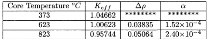
Table 2: PARCS Prompt Negative Temperature Coefficients of Reactivity

Core Temperature 'C Kef f

AP

373 1.04662 *

623 1.00623 0.03835 1.52x10-4

823 0.95744 0.05064 2.40x 10-4

Table 2 exemplifies the linear interpolation used by PARCS to calculate temperature dependent cross sections. Temperatures at which the Serpent cross sections were gen-erated were 373 "C, 623'C and 873'C.

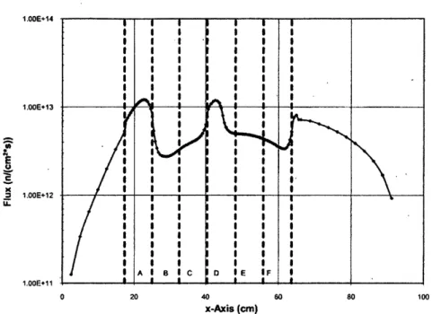
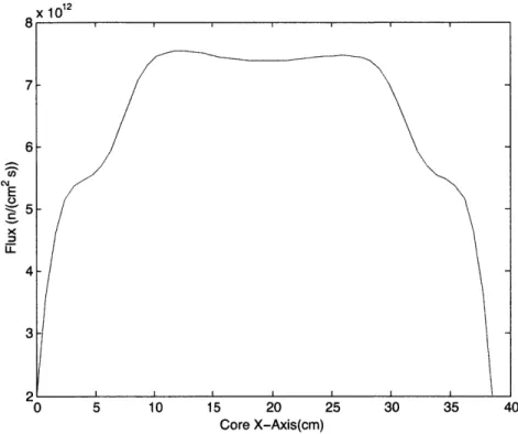
Along the x-axis (East to West) through the transient rod, the SAR's DIF3D model has a thermal flux peak in water regions just outside the core and another near the transient control rod. Figures 3 and 4 are the DIF3D and PARCS flux profiles along the x-axis, respectively.

I.OOE+14 1.OOE+13 1 C 0 .00E+12 a: 1.00E+11 I I I S I I * I I S I I I I I I I I S a s S * I I S I S I I I I I I I I I r Xi. I I a V I I 3 a I I B S I I I S I S I S -4--1ri mr r

-I

I

I

I

Figure 5: Flux profile as calculated by DIF3D; left of section "B" and to the right of "F" are outside the reactor core.

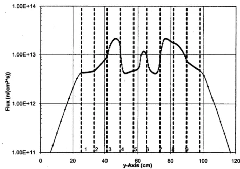
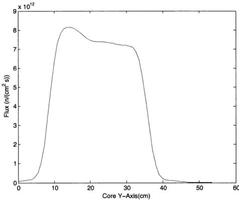
Along the y-axis,(North to South), through the transient rod, the SAR's DIF3D model has two thermal flux peaks in the two water regions, each surrounded by fuel assemblies on 3 sides. Figures 5 and 6 are the DIF3D and PARCS flux profiles along the y-axis, respectively.

x 1012 8 i- 7- 6-E 0 5-X 4- 3-2 0 5 10 15 20 25 30 35 40 Core X-Axis(cm)

Figure 6: The dimensions of this plot begins at section "B" and ends at section "F" of Figure 3.

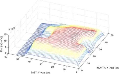
From the two dimensional plots, it appears there are no commonalities between the PARCS and DIF3D flux calculations. However looking at the PARCS three dimensional flux map, we see the thermal flux peaks observed by DIF3D in water regions adjacent to fuel flux peaks in the PARCS model.

1.OOE+14 1.OOE+13 1.OOE+12 1.00E+11 0 20 40 I I * I * I * I 60 y-AxIs (cm) I I I I 3 6 * I I I I I I I l I I I 80 100 120

Figure 7: Along the y-axis center line only regions 4, 5 and 6 contain fuel. Note that this plot is from (South to North).

x 10" 9 8- 7- 6-Em 5 -- x4-- 3-- 21 --0 0 10 20 30 40 50 60 Core Y-Axis(cm)

Figure 8: The dimensions of this plot begins at section "3" and ends at section "7" of Figure 3, (North to South).

50 V 40 0 30 60 20 50 40 1 30 1 20 10 00 NORTH, X-Axis (cm) EAST, V-Axis (cm) 0

Figure 9: The phenomenon of thermal flux peaks observed by DIF3D in water regions adjacent to fuel flux peaks in the PARCS model. This is the most pronounced along the y-axis centerline.

Transient Calculation

We are unable to construct a PARCS simulation using the correct cross-sectional data and thermal hydraulic parameters. While the model converges during transient analysis, it produces unreasonable reactivity, power, and fuel temperature figures. In particular, we find that the thermal hydraulics calculations of fuel temperatures tended toward unrealistic values before the simulation crashed. We assumed the incorrect fuel temper-atures are the cause of the reactivity and power inaccuracies.

Therefore, we removed temperature dependence from our model. However this is not ideal, as the TRIGA reactor's strong negative power coefficient is key to pulse char-acteristics. Yet, we believe a model using temperature invariant cross sections will still provide insight in the comparison of nodal and point kinetics. The fundamental differ-ences between using nodal kinetics and point kinetics should be observable regardless.

We ran a transient models where the transient control rod is removed at a linear rate (a 'ramp' control rod removal) such that it is completely removed in 1.0 seconds (38.1 cm/s). Without thermal hydraulic feedback, it is near impossible to accurately analogizes this to the Texas A&M TRIGA pulse. It is also worth noting that the core geometry had to be slightly modified to achieve convergence in the PARCS model. Figure 10 is a Serpent rendering of the new geometry.

Figures 11 and 12 are a comparison of the reactor power and reactivity versus time. The similarity in these two plots give us confidence that the PARCS nodal kinetics model and Matlab point kinetics model are simulating the same event.

For the 1.0 second transient, we compare the flux at three different times: in the middle of the pulse (0.5243 seconds), just after the transient rod has exited the core (1.0051 seconds), and well after the transient (10.0 seconds)

Figure 10: Control rods are brown, fuel is pink, graphite is light blue and water is purple.

define the "maximum percent difference" (MPD) as,

percent difference = nodalflux - pointflux (4)

nodaliux

1.0 Ramp Pulse Noda Nodal Point 0 1 2 3 4 5 Time (seconds) 6 7 8 9 10

Figure 11: As expected, reactor power grows exponentially without thermal feedback.

x10 4 3.5 -c 2.5 21.5 0.5 -u 1

= 0.4

0.3

1.0 Ramp Pulse

0 1 2 3 4 5 6 7 8 9 10

Time (seconds)

Figure 12: Similar to power, reactivity peaks just before the transient control exists the reactor core.

At 0.5243 seconds, we observe an expected difference between point and nodal ki-netics. Figure 13 depicts the point kinetics flux map, the nodal kinetics flux map and the difference of the two calculations. The nodal kinetics simulation indicated 178.26% of steady-state power, while point kinetics indicated 160.03%.

'04 a)2 E goA 100 50 0 0 _X-Axis 60 40 Y-Axis 0 0 X-Axis Y-Axis 0 0 X-Axis

Figure 13: 0.5243 seconds into the 1.0 ramp pulse. The point kinetics (top right) maintains the steady-state flux profile while nodal kinetics (top left) shows a relative increase in the assembly containing the transient control rod. Below is the difference of the flux maps. Note that the two normalized thermal flux profiles above were to scaled based on the reactor power predicted by each method, respectively. The MPD is 40.90%. M:68 a4 F2 100 Y-Axis 80 60 .5 a-V 0 z a) V_a) 0 z

From 0.5243 seconds to 1.0051 seconds, the nodal methods calculation indicates the flux peak has moved to the transient control rod from assembly E6 .

....

~-

~

~

Figure 14: At 1.0051 seconds the peak flux moves to the MPD has increased to 47.01%

the transient control rod assembly and

20-, 80 10 -87 4 - 2.-

0-From 1.0051 seconds to 10.0 seconds, the changes in both flux profiles are relatively small. The difference peak, as seen in Figure 13, is in the same location, but the MPD slightly increases to of 46.19%. At 10 seconds the point kinetics reactor power is 401.25% of steady-state while PARCS's nodal methods indicate a power of 393.52%.

2000 1500 1000. S500 8 80 8 60 . .. 60 40 40 20 20 0 0 Y-Ax~ X-Axis S 500 .. .. ... 80 0 0 Y-Axis X-Axis 1000 - -800 .... 600 . 400 200 0 ----.. --200 .... -208 80 0 60 8 40 2 .. 0... 20 40 6 0 0 Y-Axis X-Axis

In hindsight, while not having a thermal feedback is not ideal in that we cannot match calculated pulse power levels and fluxes, it also exaggerates the difference between the two schemes making the fundamental differences more readily apparent.

Conclusion

The relative closeness of the k-effective, negative temperature coefficients and 3-effective give us confidence that our model is reasonable and captures many essential character-istics of the Texas A&M TRIGA. However, there are clearly flaws in modeling such a small reactor. The phenomena of the thermal peak being outside the core at steady-state is unique and our PARCS's inability to recognize this, is perhaps one of many critical gaps limiting our model.

The discrepancy between our nodal and point kinetics would likely decrease with the incorporation of thermal feedback. However, our analysis indicates that point kinetics is fundamentally inappropriate for modeling TRIGA reactor pulses. By maintaining the steady-state flux profile, point kinetics does not capture the movement of the power peak from the E6 assembly to transient control rod assembly. This error is a cause for concern, because the largest discrepancies occur in the region surrounding the transient control rod; the same region where fuel rod deformation in the Texas A&M TRIGA reactor was observed.

Bibliography

[1] J. Remlinger, Safety Analysis Report Nuclear Science Center, Texas Engineering Experiment Station,Texas AM University System, July 2009.

[2] T. Downar, PARCS v3.0 User Manual, Department of Nuclear Engineering and Radiological Sciences University of Michigan, September 2009.

[3] T. Downar, GenPMAXS- V5, Code for Generating the PARCS Cross Section

Inter-face File PMAXS, Department of Nuclear Engineering and Radiological Sciences

University of Michigan, December 2009.

[4] J. Leppanen, PSG2

/