HAL Id: inria-00289545
https://hal.inria.fr/inria-00289545
Submitted on 21 Jun 2008
HAL is a multi-disciplinary open access
archive for the deposit and dissemination of
sci-entific research documents, whether they are
pub-lished or not. The documents may come from
teaching and research institutions in France or
L’archive ouverte pluridisciplinaire HAL, est
destinée au dépôt et à la diffusion de documents
scientifiques de niveau recherche, publiés ou non,
émanant des établissements d’enseignement et de
recherche français ou étrangers, des laboratoires
Coinductive big-step operational semantics
Xavier Leroy
To cite this version:
Xavier Leroy. Coinductive big-step operational semantics. European Symposium on Programming
(ESOP 2006), Mar 2006, Vienne, Austria. pp.42-54, �10.1007/11693024_5�. �inria-00289545�
Coinductive big-step operational semantics
Xavier Leroy INRIA Rocquencourt
Domaine de Voluceau, B.P. 105, 78153 Le Chesnay, France [email protected]
Abstract. This paper illustrates the use of coinductive definitions and proofs in big-step operational semantics, enabling the latter to describe diverging evaluations in addition to terminating evaluations. We show applications to proofs of type soundness and to proofs of semantic preser-vation for compilers.
1
Introduction
There exist two popular styles of structured operational semantics: big-step se-mantics, relating programs to final configurations, and small-step sese-mantics, where a one-step reduction relation is repeatedly applied to form reduction se-quences. Small-step semantics is more expressive since it can describe the eval-uation of both terminating and non-terminating programs, as finite or infinite reduction sequences, respectively. In contrast, big-step semantics describes only the evaluation of terminating programs, and fails to distinguish between non-terminating programs and programs that “go wrong”. For this reason, small-step semantics is generally preferred, in particular for proving the soundness of type systems.
However, big-step semantics is more convenient than small-step semantics for some applications. One that is dear to our heart is proving the correct-ness (preservation of program behaviours) of program transformations, espe-cially compilation of a high-level language down to a lower-level language. Our experience and that of others [14, 12, 19] is that fairly complex, optimizing com-pilation passes can be proved correct relatively easily using big-step semantics, by induction on the structure of big-step evaluation derivations. In contrast, compiler correctness proofs using small-step semantics are significantly harder even for simple, non-optimizing compilation schemes [10, 8].
In this paper, we illustrate how coinductive definitions and proofs enable big-step semantics to describe both finite and infinite evaluations. The target of our study is a simple call-by-value functional language. We study two ap-proaches: the first, initially proposed by Cousot and Cousot [4], complements the normal inductive big-step evaluation rules for finite evaluations with coin-ductive big-step rules describing diverging evaluations; the second simply inter-prets coinductively the normal big-step evaluation rules, thus enabling them to describe both terminating and non-terminating evaluations. These semantics are
defined in section 2. The main technical results of the paper are: connections be-tween coinductive big-step semantics and finite or infinite reduction sequences in small-step semantics (section 3); a novel approach to stating and proving the soundness of type systems (section 4); and proofs of semantic preservation for compilation down to an abstract machine (section 5).
An originality of this paper is that all results were not only proved using a proof assistant (the Coq system), but even developed in interaction with this tool, and only then transcribed to standard mathematical notations in this pa-per. The Coq proof assistant [3] provides built-in support for coinductive def-initions and proofs by a limited form of coinduction called guarded structural coinduction. (See [6, 2, 3] for descriptions of this approach to coinduction.) Such proofs are easier than the standard, on-paper proofs by coinduction; in partic-ular, there is no need to exhibit F -consistent relations [5]. This enables us to play fast and loose with coinduction in the proof sketches given in this paper; the skeptical reader is referred to the corresponding Coq development [13] for details. Another benefit of using Coq is that our formalization and proofs use rather modest mathematics: just syntactic definitions, no domain theory, and constructive logic plus the axiom of excluded middle from classical logic. (The proofs that use excluded middle are marked “classical ”.)
2
The language and its big-step semantics
The language we consider in this paper is the λ-calculus extended with constants: the simplest functional language that exhibits run-time errors (terms that “go wrong”). Its syntax is as follows:
Variables: x, y, z, . . .
Constants: c::= 0 | 1 | . . . Terms: a, b, v::= x | c | λx.a | a b
We write a[x ← b] for the capture-avoiding substitution1 of b for all free
occur-rences of x in a. We say that a term v is a value, and write v ∈ Values, if a is either a constant c or an abstraction λx.b.
The standard call-by-value semantics in big-step style for this language is defined by the following inference rules, interpreted inductively.
c⇒ c (⇒-const) λx.a⇒ λx.a (⇒-fun) a1⇒ λx.b a2⇒ v2 b[x ← v2] ⇒ v
(⇒-app) a1 a2⇒ v
More precisely, the relation a ⇒ v (read: “a evaluates to v”) is the smallest fixpoint of the rules above. Equivalently, a ⇒ v holds if and only if it is the conclusion of a finite derivation tree built from the rules above.
1 The Coq development does not treat terms modulo α-conversion, therefore the
sub-stitution a[x ← b] is capture-avoiding only if b is closed. However, this suffices to define evaluation and reduction of closed source terms.
Lemma 1. If a ⇒ v, then v ∈ Values.
Proof sketch. Induction on the derivation of a ⇒ v.
The rules above capture only terminating evaluations. Writing δ = λx. x x and ω = δ δ, we have for instance:
Lemma 2. ω⇒ v is false for all terms v.
Proof sketch. We show that a ⇒ v implies a 6= ω by induction on the derivation of a ⇒ v.
Following Cousot and Cousot [4] and more recent work by Grall [7], we de-fine divergence (infinite evaluations) by the following inference rules, interpreted coinductively:2 a1 ∞ ⇒ (⇒-app-l)∞ a1a2 ∞ ⇒ a1⇒ v a2 ∞ ⇒ (⇒-app-r)∞ a1 a2 ∞ ⇒ a1⇒ λx.b a2⇒ v b[x ← v] ∞ ⇒ (⇒-app-f)∞ a1a2 ∞ ⇒
More precisely, the relation a ⇒ (read: “a diverges”) is the greatest fixpoint∞ of the rules above, or, equivalently, the conclusions of infinite derivation trees built from these rules. Note that we have imposed (arbitrarily) a left-to-right evaluation order for applications.
Lemma 3. ω⇒ holds.∞
Proof sketch. By coinduction. Assume ω⇒ as coinduction hypothesis. We can∞ derive ω ⇒ with rule (∞ ⇒-app-f), using the coinduction hypothesis as third∞ premise.
Lemma 4. a⇒ v and a⇒ are mutually exclusive.∞
Proof sketch. By induction on the derivation of a ⇒ v and inversion on a⇒ .∞ An alternate attempt to describe both terminating and non-terminating eval-uations at the same time is to interpret coinductively the standard evaluation rules for terminating evaluations.
c⇒ c (co ⇒-const)co λx.a⇒ λx.a (co ⇒-fun)co a1 co ⇒ λx.b a2 co ⇒ v2 b[x ← v2] co ⇒ v (⇒-app)co a1 a2 co ⇒ v
2 Throughout this paper, double horizontal lines in inference rules denote inference
rules that are to be interpreted coinductively; single horizontal lines denote the inductive interpretation.
The relation a⇒ b (read: “a coevaluates to b”) is therefore the greatest fixpointco of the standard evaluation rules. It holds if and only if a⇒ b is the conclusionco of a finite or infinite derivation tree built from these rules.
Naively, we could expect that⇒ is the union of ⇒ andco ∞
⇒. This intuition is supported by the following properties:
Lemma 5. If a ⇒ v, then a⇒ v.co
Proof sketch. By induction on the derivation of a ⇒ v. Lemma 6. ω⇒ v for all terms v.co
Proof sketch. By coinduction, using rule (⇒-app) with the coinduction hypoth-co esis as third premise.
Lemma 7. If a⇒ v, then either a ⇒ v or aco ⇒ .∞
Proof sketch (classical). We show that a⇒ v and ¬(a ⇒ v) implies aco ⇒ . The∞ result then follows by excluded middle on a ⇒ v. The auxiliary property is proved by coinduction and case analysis on a. The cases for variables, constants and abstractions trivially contradict one of the hypotheses. If a = a1a2, inversion
on the hypothesis a⇒ v shows that aco 1 co ⇒ λx.b and a2 co ⇒ v2and b[x ← v2] co ⇒ v. Using excluded middle, it must be that at least one of these three terms does not evaluate, otherwise, a ⇒ v would hold. The result follows by applying the rule for ⇒ that matches which term does not evaluate, and using the coinduction∞ hypothesis.
However, the reverse implication does not hold: there exists terms that di-verge but do not coevaluate. Consider for instance a = ω (0 0). It is true that a⇒ , but there is no term v such that a∞ ⇒ v, because the coevaluation of theco argument 0 0 goes wrong (there is no v such that 0 0⇒ v).co
Another unusual feature of coevaluation is that it is not deterministic. For instance, ω ⇒ v for any term v. However,co ⇒ is deterministic for terminatingco terms, in the following sense:
Lemma 8. If a ⇒ v and a⇒ vco ′
, then v′
= v.
Proof sketch. By induction on the derivation of a ⇒ v and inversion on a⇒ vco ′
. Moreover, there exists diverging terms that coevaluate to only one value. An example is (λx.0) ω, which coevaluates to 0 but not to any other term.
3
Relation with small-step semantics
The one-step reduction relation → is defined by the call-by-value β-reduction axiom plus two context rules for reducing under applications, assuming left-to-right evaluation order.
v∈ Values (→-β) (λx.a) v → a[x ← v] a1→ a2 (→-app-l) a1 b→ a2 b a∈ Values b1→ b2 (→-app-r) a b1→ a b2
There are three kinds of reduction sequences of interest. The first, written a → b (“a reduces to b in zero, one or several steps”), is the normal reflexive∗ transitive closure of →; it captures finite reductions. The second, a→ (“a re-∞ duces infinitely”) captures infinite reductions. The third, aco∗→ b (“a reduces to b in zero, one, several or infinitely many steps”) is the coinductive interpretation of the rules for reflexive transitive closure; it captures both finite and infinite reduc-tions. These relations are defined by the following rules, interpreted inductively for→ and coinductively for∗ → and∞ co∗→.
a→ a∗ aco∗→ a a→ b b→ c∗ a→ c∗ a→ b b→∞ a→∞ a→ b bco∗→ c aco∗→ c
In contrast with the evaluation predicates of section 2, it is true thatco∗→ is the union of→ and∗ →.∞
Lemma 9. aco∗→ b if and only if a→ b or a∗ → .∞
Proof sketch (classical). For the “if” part, we show that a→ b =⇒ a∗ co∗→ b by induction on a → b, and that a∗ → =⇒ a∞ co∗→ b by coinduction. For the “only if” part, we show that aco∗→ b ∧ ¬(a→ b) =⇒ a∗ → by coinduction. The result∞ follows by excluded middle over a→ b.∗
We now turn to relating the reduction relations (small-step) and the evalua-tion relaevalua-tions (big-step). (Some of these results were proved earlier on paper by Grall [7], using a variant of the F -consistent relation approach.) It is well known that normal evaluation is equivalent to finite reduction to a value:
Lemma 10. a⇒ v if and only if a→ v and v ∈ Values.∗
Proof sketch. The “only if” part is an easy induction on a ⇒ v. For the “if” part, we first show the following two lemmas: (1) v ⇒ v if v ∈ Values, and (2) a⇒ v if a → b and b ⇒ v. The result follows by induction on the derivation of a→ v.∗
Similarly, divergence (⇒) is equivalent to infinite reduction (∞ →). The proof∞ uses the following lemma:
Lemma 11. For all terms a, either a→ , or there exists b such that a∞ ∗
→ b and b6→, that is, ∀c, ¬(b → c).
Proof sketch (classical). We first show that ∀b, a → b =⇒ ∃c, b → c implies∗ a→ by coinduction. We then argue by excluded middle on a∞ → .∞
Lemma 12. a⇒ if and only if a∞ → .∞
Proof sketch (classical). For the “only if” part, we first show that a⇒ implies∞ ∃b, a → b ∧ b⇒ by structural induction on a, then conclude by coinduction.∞ For the “if” part, we proceed by coinduction and case analysis over a. The only non-trivial case is a = a1 a2. Using lemma 11, we distinguish three cases: (1) a1
reduces infinitely; (2) a1reduces to a value but a2 reduces infinitely; (3) a1 and
reduce to values λx.b and v respectively, and b[x ← v] reduces infinitely. The result a⇒ then follows from the coinduction hypothesis in all three cases.∞
For coevaluations⇒ and coreductionsco co∗→, the equivalence holds in one di-rection only.
Lemma 13. a⇒ v implies aco co∗→ v.
Proof sketch. Using classical logic, this follows from lemmas 7, 10, 12 and 9. However, the result can be proved directly in constructive logic. We first show that a⇒ v =⇒ a ∈ Values ∨ ∃b, a → b ∧ bco ⇒ v by induction on a. The resultco follows by coinduction.
An example where the reverse implication does not hold is a = (λx. 0) ω and v= 1. Since a→ , we have a∞ co∗→ v. However, a⇒ v does not hold since the onlyco term to which a coevaluates is 0.
4
Type soundness proofs
We now turn to using our coinductive evaluation and reduction relations for proving the soundness of type systems. To be more specific, we will use the simply-typed λ-calculus with recursive types as our type system. We obtain re-cursive types by interpreting the type algebra τ ::= int | τ1→ τ2 coinductively,
as in [5]. The typing rules are recalled below. Γ ranges over type environments, that is, finite maps from variables to types.
E(x) = τ E⊢ x : τ E⊢ c : int E+ {x : τ′ } ⊢ a : τ E⊢ λx.a : τ′ → τ E⊢ a1: τ′ → τ E ⊢ a2: τ′ E⊢ a1a2: τ
Enabling recursive types makes the type system non-normalizing and allows interesting programs to be written. In particular, the call-by-value fixpoint op-erator Y = λf. (λx. f (x x)) (λx. f (λy. (x x) y)) is well-typed, with types ((τ → τ′
) → τ → τ′
) → τ → τ′
for all types τ , τ′
4.1 Type soundness proofs using small-step semantics
Felleisen and Wright [20] introduced a proof technique for showing type sound-ness that relies on small-step semantics and is standard nowadays. The proof relies on the twin properties of type preservation (also called subject reduction) and progress:
Lemma 14 (Preservation). If a → b and ∅ ⊢ a : τ , then ∅ ⊢ b : τ Lemma 15 (Progress). If ∅ ⊢ a : τ , then either a ∈ Values or ∃b, a → b.
The formal statement of type soundness in Felleisen and Wright’s approach is the following:
Lemma 16 (Type soundness, 1). If ∅ ⊢ a : τ and a → b, then either a ∈∗ Values or there exists b such that a → b.
Proof sketch. We first show that ∅ ⊢ b : τ by induction over a → b, using the∗ preservation lemma. We then conclude with the progress lemma.
Authors that follow this approach then conclude that well-typed closed terms either reduce to a value or reduce infinitely. However, this conclusion is generally not expressed nor proved formally. In our approach, it is easy to do so:
Lemma 17 (Type soundness, 2). If ∅ ⊢ a : τ , then either a → , or there∞ exists v such that a→ v and v ∈ Values.∗
Proof sketch (classical). By lemma 11, either a → or ∃v, a∞ → v ∧ v 6→. The∗ result is obvious in the first case. In the second case, we note that ∅ ⊢ v : τ as a consequence of the preservation lemma, then use the progress lemma to conclude that v ∈ Values.
An alternate, equivalent formulation of this theorem uses the coreduction relationco∗→.
Lemma 18 (Type soundness, 3). If ∅ ⊢ a : τ , then there exists v such that aco∗→ v and v ∈ Values.
Proof sketch (classical). Follows from lemmas 17 and 9.
An arguably nicer characterisation of “programs that do not go wrong” is given by the relation asafe→ (read: “a reduces safely”), defined coinductively by the following rules:
v∈ Values vsafe→
a→ b bsafe→ asafe→
These rules are interpreted coinductively so that a safe→ holds if a reduces in-finitely. We can then state and show type soundness without recourse to classical logic:
Lemma 19 (Type soundness, 4). If ∅ ⊢ a : τ , then asafe→ .
Proof sketch. By coinduction. Applying the progress lemma, either a ∈ Values and we are done, or a → b for some b. In the latter case, ∅ ⊢ b : τ by the preservation property, and the result follows from the coinduction hypothesis.
4.2 Type soundness proofs using big-step semantics
The standard big-step semantics (the ⇒ relation) is awkward for proving type soundness because it does not distinguish between terms that diverge and terms that go wrong: in both cases, there is no value v such that a ⇒ v. Consequently, the obvious type soundness statement “if ∅ ⊢ a : τ , there exists v such that a⇒ v” is false for all type systems that do not guarantee normalization. The best result we can prove, then, is the following big-step equivalent to the preservation lemma:
Lemma 20. If a ⇒ v and ∅ ⊢ a : τ , then ∅ ⊢ v : τ .
The standard approach is to provide inductive inference rules to define a predicate a ⇒ err characterizing terms that go wrong, and prove the weaker type soundness statement “if ∅ ⊢ a : τ , then it is not the case that a ⇒ err”. This approach is unsatisfactory for two reasons: (1) extra rules must be provided to define a ⇒ err, which increases the size of the semantics; (2) there is a risk that the rules for a ⇒ err are incomplete and miss some cases of “going wrong”, in which case the type soundness statement does not guarantee that well-typed terms either evaluate to a value or diverge.
Let us revisit these trade-offs in the light of our characterizations of diver-gence and coevaluation. We can now formally state what it means for a term to evaluate or to diverge. This leads to the following alternate statement of type soundness:
Lemma 21 (Type soundness, 5). If ∅ ⊢ a : τ , then either a ⇒ or there∞ exists v such that a ⇒ v.
This result follows from the lemma below (a big-step analogue to the progress lemma) and from excluded middle applied to ∃v. a ⇒ v.
Lemma 22. If ∅ ⊢ a : τ and ∀v, ¬(a ⇒ v), then a⇒ .∞
Proof sketch (classical). The proof is by coinduction and case analysis over a. The cases a = x, a = c and a = λx.b lead to contradictions: variables are not typeable in the empty environment; constants and abstractions evaluate to themselves. The interesting case is therefore a = a1 a2. By excluded middle,
either a1evaluates to some value v1, or not. In the latter case, a ∞
rule (⇒-app-l) and from a∞ 1 ∞
⇒ , which we obtain by coinduction hypothesis. In the former case, v1 has a function type τ′ → τ by lemma 20, and therefore
v1 = λx.b for some x and b. Moreover, {x : τ′} ⊢ b : τ . Using excluded middle
again, either a2 evaluates to some value v2, or not. In the latter case, a ∞
⇒ follows from rule (⇒-app-r) and the coinduction hypothesis. In the former case,∞ ∅ ⊢ v2 : τ
′
. Since typing is stable by substitution, ∅ ⊢ b[x ← v2] : τ . Using
excluded middle for the third time, it must be that ∀v. ¬(b[x ← v2] ⇒ v),
otherwise a would evaluate to some value. The result a ⇒ then follows from∞ rule (⇒-app-f) and the coinduction hypothesis.∞
The proof above is an original alternative to the standard approach of show-ing ¬(a ⇒ err) for all well-typed terms a. From a methodological standpoint, our proof addresses one of the shortcomings of the standard approach, namely the risk of not putting enough error rules. If we forget some divergence rules, the proof of lemma 22 will, in all likelihood, not go through. Moreover, it is improbable to put too many rules for divergence and still have the property that a⇒ v and a∞
⇒ are mutually exclusive. Therefore, this novel approach to prov-ing type soundness usprov-ing big-step semantics appears rather robust with respect to mistakes in the specification of the semantics.
The other methodological shortcoming remains, however: just like the “not goes wrong” approach, our approach requires more evaluation rules than just those for normal evaluations, namely the rules for divergence. This can easily double the size of the specification of a dynamic semantics, which is a serious concern for realistic languages where the normal evaluation rules number in dozens.
The coevaluation relation⇒ is attractive for these pragmatic reasons, as itco has the same number of rules as normal evaluation. Of course, we have seen that a⇒ v is not equivalent to a ⇒ v ∨ aco ⇒ , but the example we gave was for a∞ term a that is not typeable and where an early diverging evaluation “hides” a later evaluation that goes wrong. Since type systems ensure that all subterms of a term do not go wrong, we could hope that the following conjecture holds: Conjecture 1 (Type soundness, 6). If ∅ ⊢ a : τ , there exists v such that a⇒ v.co
We were able to prove this conjecture for some uninteresting but nonetheless non-normalizing type systems, such as simply-typed λ-calculus without recur-sive types, but with a predefined constant of type int → int that diverges when applied. However, the conjecture is false for simply-typed λ-calculus with recur-sive types, and probably for all type systems with a general fixpoint operator. Andrzej Filinski provided the following counterexample. Consider
Y F 0 where F = λf.λx. (λg.λy. g y) (f x).
The term Y F 0 is well-typed with type int → int, yet it fails to coeval-uate: the only possible value v such that Y F 0 ⇒ v is an infinite term,co λy.(λy. (λy. . . . y) y) y.
5
Compiler correctness proofs
We now return to the original motivation of this work: proving semantic preser-vation for compilers both for terminating and diverging programs, using big-step semantics. We demonstrate this approach on the compilation of call-by-value λ-calculus down to a simple abstract machine.
5.1 Big-step semantics with environments and closures
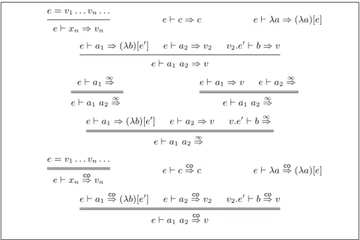
e= v1. . . vn. . . e ⊢ xn⇒ vn e ⊢ c ⇒ c e ⊢ λa ⇒(λa)[e] e ⊢ a1⇒(λb)[e′ ] e ⊢ a2⇒ v2 v2.e′ ⊢ b ⇒ v e ⊢ a1 a2⇒ v e ⊢ a1⇒∞ e ⊢ a1a2⇒∞ e ⊢ a1⇒ v e ⊢ a2⇒∞ e ⊢ a1 a2⇒∞ e ⊢ a1 ⇒(λb)[e′ ] e ⊢ a2⇒ v v.e′ ⊢ b⇒∞ e ⊢ a1a2⇒∞ e= v1. . . vn. . . e ⊢ xn co ⇒ vn e ⊢ c⇒ cco e ⊢ λa⇒co (λa)[e] e ⊢ a1⇒co (λb)[e′ ] e ⊢ a2⇒ vco 2 v2.e′ ⊢ b⇒ vco e ⊢ a1 a2⇒ vco
Fig. 1.Big-step evaluation rules with closures and environments
Our abstract machine uses closures and environments indexed by de Bruijn indices. It is therefore convenient to reformulate the big-step evaluation predi-cates in these terms. Variables, written xn, are now identified by their de Bruijn
indices n. Values (which are no longer a subset of terms) and environments are defined as:
Values: v::= c integer values | (λa)[e] function closures Environments: e ::= ε | v.e sequences of values
Figure 1 shows the inference rules defining the three evaluation relations: e⊢ a ⇒ v finite evaluations (inductive)
e⊢ a⇒∞ infinite evaluations (coinductive) e⊢ a⇒ vco coevaluations (coinductive)
We will not formally study these relations, but note that they enjoy the same properties as the environment-less relations studied in section 2.
5.2 The abstract machine and its compilation scheme
The abstract machine we use as target of compilation follows the call-by-value strategy and the “eval-apply” model. It is close in spirit to the SECD, CAM, FAM and CEK machines. The machine state has three components: a code sequence, a stack and an environment. The syntax for these components is as follows.
Instructions: I::= Var(n) push the value of variable number n | Const(c) push the constant c
| Clos(C) push a closure for code C | App perform a function application | Ret return to calling function Code: C::= ε | I, C instruction sequences Machine values: V ::= n integer values
| C[E] code closures Machine environments: E ::= ε | V.E
Stacks: S::= ε empty stack | V.S pushing a value | (C, E).S pushing a return frame
The behaviour of the abstract machine is defined by the following rules, as a transition relation C; S; E → C′
; S′
; E′
that relates the machine state before (C; S; E) and after (C′
; S′
; E′
) the execution of the first instruction of the code C.
(Var(n), C); S; E → C; Vn.S; E if E = V1. . . Vn. . . (Const(c), C); S; E → C; c.S; E (Clos(C′ ), C); S; E → C; C′ [E].S; E (App, C); V.C′ [E′ ].S; E → C′ ; (C, E).S; V.E′ (Ret, C); V.(C′ , E′ ).S; E → C′ ; V.S; E′
As in section 3, we consider the following closures of the one-step transition relation:
C; S; E → C∗ ′
; S′
; E′
zero, one or several transitions (inductive) C; S; E → C+ ′
; S′
; E′
one or several transitions (inductive) C; S; E →∞ infinitely many transitions (coinductive) C; S; E co∗→ C′
; S′
; E′
zero, one, several or infinitely many transitions (coind.) The compilation scheme from terms to code is straightforward:
[[xn]] = Var(n) [[c]] = Const(c)
The intended effect for the code [[a]] is to evaluate the term a and push its value at the top of the machine stack, leaving the rest of the stack and the environment unchanged.
5.3 Proofs of semantic preservation
We expect the compilation to abstract machine code to preserve the semantics of the source term, in the following general sense. Consider a closed term a and start the abstract machine in the initial state corresponding to a. If a diverges, the machine should perform infinitely many transitions. If a evaluates to the value v, the machine should reach a final state corresponding to v in a finite number of transitions. Here, the initial state corresponding to a is [[a]]; ε; ε. The final state corresponding to the result value v is ε; [[v]].ε; ε, that is, the code has been entirely consumed and the machine value [[v]] corresponding to the source-level value v is left on top of the stack. The correspondence between source-source-level and machine values is defined by:
[[c]] = c [[(λa)[e]]] = ([[a]], Ret)[[[e]]] [[v1. . . vn]] = [[v1]] . . . [[vn]]
Semantic preservation is easy to show for terminating terms a using the big-step semantics. We just need to strengthen the statement of preservation so that it lends itself to induction over the derivation of e ⊢ a ⇒ v. (See the Coq development [13] for the full proof.)
Lemma 23. If e ⊢ a ⇒ v, then ([[a]], C); S; [[e]]→ C; [[v]].S; [[e]] for all codes+ C and stacks S.
It is impossible, however, to prove semantic preservation for diverging terms using only the standard big-step semantics. This led several authors to prove semantic preservation for compilation to abstract machines using small-step se-mantics with explicit substitutions [10, 17]. Such proofs are difficult, however, because the obvious simulation property
If a[e] → a′
[e′
] then [[a]]; S; [[e]]→ [[a+ ′
]]; S′
; [[e′
]] (for some S′
)
does not hold: the transitions of the abstract machine do not follow the reduc-tions of the source term. Instead, the proofs in [10, 17] rely on a decompilation relation that maps intermediate machine states back to source-level terms. With the help of this decompilation relation, it is possible to prove simulation diagrams that imply the desired semantic preservation properties. However, decompilation relations are difficult to define, especially for optimizing compilation schemes (see [8] for an example).
The coinductive big-step semantics studied in this paper provide a simpler way to prove semantic preservation for non-terminating terms. Namely, the fol-lowing two theorems hold, showing that compilation preserves divergence and coevaluation as characterized by the⇒ and∞ ⇒ predicates.co
Lemma 25. If e ⊢ a⇒ v, then ([[a]], C); S; [[e]]co co∗→ C; [[v]].S; [[e]].
The full proofs can be found in [13]. Both lemmas cannot be proved directly by structural coinduction and case analysis over a. The problem is in the appli-cation case a = a1a2, where the code component of the initial machine state is of
the form [[a1]], [[a2]], App, C. It is not possible to invoke the coinduction hypothesis
to reason over the execution of [[a1]], because this use of the coinduction
hypoth-esis is not guarded by an inference rule for the → relation, or in other terms∞ because no machine instruction is evaluated before invoking the hypothesis.
There are two ways to address this issue. The first is to modify the compi-lation scheme for applications, in order to insert a “no operation” instruction in front of the generated sequence: [[a1 a2]] = Nop, [[a1]], [[a2]]. The Nop operation
has the obvious machine transition (Nop, C); S; E → C; S; E. With this mod-ification, the coinductive proof for lemma 24 performs a Nop transition before invoking the coinduction hypothesis to deal with the evaluation of [[a1]]. This
makes the coinductive proof properly guarded and acceptable to Coq.
Of course, it is inelegant to pepper the generated code with Nop instructions just to make one proof get through. We therefore used an alternate approach where the compilation scheme for applications is unchanged, but we exploit the fact that the number of such recursive calls that do not perform a machine transition is necessarily finite, because our term algebra is finite. The proof of lemma 24 exploits this fact by defining a variant of the→ relation that enables a∞ finite number of “stuttering steps” (where no instructions are executed) between executions of instructions. The finite number in question is the length of the left application spine of the term being compiled. The problem and the solution are similar to those described by Bertot [2] in his coinductive presentation and proof of Eratosthenes’ sieve algorithm.
6
Related work
There are few instances of coinductive definitions and proofs for big-step seman-tics in the literature. Cousot and Cousot [4] proposed the coinductive big-step characterization of divergence that we use in this paper and studied its applica-bility for abstract interpretation. Grall [7] applied this approach to call-by-value λ-calculus; unlike our ⇒ and⇒ predicates, his big-step semantics also generate∞ finite or infinite traces of elementary computation steps, traces which he uses to define observational equivalences. Gunter and R´emy [9] and Stoughton [18] have the same initial goal as us, namely describe both terminating and diverg-ing computations with big-step semantics, but use increasdiverg-ing sequences of finite, incomplete derivations to do so, instead of infinite derivations. We do not know yet how their approach relates to our⇒ and∞ ⇒ relations.co
Milner and Tofte [16] and later Leroy and Rouaix [15] used coinduction in the context of a big-step semantics for functional and imperative languages, not to describe diverging evaluations, but to capture safety properties over possibly cyclic memory stores.
Of course, coinductive techniques are routinely used in the context of small-step semantics, especially for the labeled transition systems arising from process calculi. The flavours of coinduction used there, especially proofs by bisimulations, are quite different from the present work.
The infinitary λ-calculus [11, 1] studies diverging computations from a very different angle: not only the authors use reduction semantics, but their terms are also infinite, and they use topological tools (metrics, convergence, etc) instead of coinduction.
7
Conclusions
We investigated two coinductive approaches to giving big-step semantics for non-terminating computations. The first, based on [4] and using separate evaluation rules for terminating terms and diverging terms, appears very well-behaved: it corresponds exactly to finite and infinite reduction sequences, and lends itself well to type soundness proofs and to compiler correctness proofs. The second approach, consisting in a coinductive interpretation of the standard evaluation rules, is less satisfactory: while amenable to compiler correctness proofs as well, it captures only a subset of the diverging computations of interest — and it is not yet clear which subset exactly.
A natural continuation of this work, following Grall’s work [7], is to develop coinductive, big-step, trace semantics for imperative languages that capture not only the final outcome of the evaluation (divergence or result value), but also a possibly infinite trace of the observable effects (such as input/output) performed during evaluation. Such trace semantics would enable stronger statements of observational equivalence between source code and compiled code in the context of compiler certification. However, the existence of suitable traces for infinite evaluations cannot be proved constructively, nor with just the axiom of excluded middle. It is not clear yet what classical axioms (probably variants of the axiom of choice) need to be added to Coq.
Acknowledgments
Andrzej Filinski disproved the conjecture from section 4.2 very shortly after it was stated. We thank the anonymous reviewers and the participants of the 22nd meeting of IFIP Working Group 2.8 (Functional Programming) for their feedback.
References
1. A. Berarducci and M. Dezani-Ciancaglini. Infinite lambda-calculus and types. Theor. Comp. Sci., 212(1-2):29–75, 1999.
2. Y. Bertot. Filters on coinductive streams, an application to Eratosthenes’ sieve. In Typed Lambda Calculi and Applications (TLCA’05), volume 3461 of LNCS, pages 102–115. Springer-Verlag, 2005.
3. Y. Bertot and P. Cast´eran. Interactive Theorem Proving and Program Development – Coq’Art: The Calculus of Inductive Constructions. EATCS Texts in Theoretical Computer Science. Springer-Verlag, 2004.
4. P. Cousot and R. Cousot. Inductive definitions, semantics and abstract interpre-tation. In 19th symp. Principles of Progr. Lang, pages 83–94. ACM Press, 1992. 5. V. Gapeyev, M. Levin, and B. Pierce. Recursive subtyping revealed. J. Func.
Progr., 12(6):511–548, 2003.
6. E. Gim´enez. Codifying guarded definitions with recursive schemes. In Types for Proofs and Programs. International Workshop TYPES ’94, volume 996 of LNCS, pages 39–59. Springer-Verlag, 1994.
7. H. Grall. Deux crit`eres de s´ecurit´e pour l’ex´ecution de code mobile. PhD thesis, ´
Ecole Nationale des Ponts et Chauss´ees, Dec. 2003.
8. B. Gr´egoire. Compilation des termes de preuves: un (nouveau) mariage entre Coq et OCaml. PhD thesis, University Paris 7, 2003.
9. C. A. Gunter and D. R´emy. A proof-theoretic assessment of runtime type errors. Research Report 11261-921230-43TM, AT&T Bell Laboratories, 1993.
10. T. Hardin, L. Maranget, and B. Pagano. Functional runtimes within the lambda-sigma calculus. Journal of Functional Programming, 8(2):131–176, 1998.
11. R. Kennaway, J. W. Klop, M. R. Sleep, and F.-J. de Vries. Infinitary lambda calculus. Theor. Comp. Sci., 175(1):93–125, 1997.
12. G. Klein and T. Nipkow. A machine-checked model for a Java-like language, virtual machine and compiler. Technical Report 0400001T.1, National ICT Australia, Mar. 2004. To appear in ACM TOPLAS.
13. X. Leroy. Coinductive big-step operational semantics – the Coq development. Available from pauillac.inria.fr/~xleroy, 2005.
14. X. Leroy. Formal certification of a compiler back-end, or: programming a compiler with a proof assistant. In 33rd symp. Principles of Progr. Lang, pages 42–54. ACM Press, 2006.
15. X. Leroy and F. Rouaix. Security properties of typed applets. In J. Vitek and C. Jensen, editors, Secure Internet Programming – Security issues for Mobile and Distributed Objects, volume 1603 of LNCS, pages 147–182. Springer-Verlag, 1999. 16. R. Milner and M. Tofte. Co-induction in relational semantics. Theor. Comp. Sci.,
87:209–220, 1991.
17. M. Rittri. Proving the correctness of a virtual machine by a bisimulation. Licentiate thesis, G¨oteborg University, 1988.
18. A. Stoughton. An operational semantics framework supporting the incremental construction of derivation trees. In Second Workshop on Higher-Order Operational Techniques in Semantics (HOOTS II), volume 12 of Electronic Notes in Theoretical Computer Science. Elsevier, 1998.
19. M. Strecker. Compiler verification for C0. Technical report, Universit´e Paul Sabatier, Toulouse, April 2005.
20. A. K. Wright and M. Felleisen. A syntactic approach to type soundness. Inf. and Comp., 115(1):38–94, 1994.