HAL Id: hal-01320734
https://hal.archives-ouvertes.fr/hal-01320734
Submitted on 24 May 2016
HAL is a multi-disciplinary open access
archive for the deposit and dissemination of
sci-entific research documents, whether they are
pub-lished or not. The documents may come from
teaching and research institutions in France or
abroad, or from public or private research centers.
L’archive ouverte pluridisciplinaire HAL, est
destinée au dépôt et à la diffusion de documents
scientifiques de niveau recherche, publiés ou non,
émanant des établissements d’enseignement et de
recherche français ou étrangers, des laboratoires
publics ou privés.
Graphical characterization of the set of all flat outputs
for structured linear discrete-time systems
Taha Boukhobza, Gilles Millérioux
To cite this version:
Taha Boukhobza, Gilles Millérioux. Graphical characterization of the set of all flat outputs for
struc-tured linear discrete-time systems. 6th Symposium on System Structure and Control, SSSC 2016, Jun
2016, Istanbul, Turkey. �hal-01320734�
Graphical characterization of the set of all
flat outputs for structured linear
discrete-time systems
Taha Boukhobza∗,∗∗ Gilles Mill´erioux∗,∗∗
∗Universit´e de Lorraine, Centre de Recherche en Automatique de
Nancy, UMR 7039, Vandoeuvre-l`es-Nancy, F-54506, France (e-mail: {taha.boukhobza, gilles.millerioux}@univ-lorraine.fr.
∗∗CNRS, Centre de Recherche en Automatique de Nancy, UMR 7039,
Vandoeuvre-l`es-Nancy, F-54506, France
Abstract: This paper deals with the characterization of flat outputs for structured linear discrete-time systems. More precisely, considering a structured discrete-discrete-time linear system, we provide a complete set of the flat outputs using constructive polynomial complexity order algorithms. The proposed method is simple to implement. It is based on usual algorithms dedicated to the computation of successors and predecessors of vertex subsets and to the computation and the ordering of strongly connected components in a digraph.
Keywords: Flatness, Structured Linear Discrete-Time Systems, Structural Analysis, Graphs.
1. INTRODUCTION
Flatness is a control-theoretical concept introduced in Fliess et al. (1995). For a flat continuous-time system, flatness is equivalent to a complete parametrization of all system variables (inputs and states) in terms of a finite number of independent variables and a finite number of their time derivatives. Those variables are called flat outputs. For discrete-time systems, a specific treatment must be considered insofar as derivatives are replaced by shifted outputs. Hence, for a flat system, the state variable as well as the input of discrete-time systems can be written as some function of the output (including for-ward and backfor-ward shifts in the output). Flatness-based control has been involved in many applications and has an outstanding interest in trajectory planning (Meurer (20114), Chamseddine et al. (2012)), predictive control and constraint handling (Don´a et al. (2009),Kandler et al. (2012)). For discrete-time systems, it has been investigated in a much lesser extent in comparison with continuous-time systems. As some exceptions, we can quote Mill´erioux et al. (2009),Parriaux et al. (2013), Sato (2012) and Kaldmae et al. (2013).
The point is that flatness-based control requires the knowl-edge of the flat outputs of the system. There exist substan-tial results for checking whether or not a given output is a flat output. On the other hand, the characterization of the set of all flat outputs for a given system is a challeng-ing problem. A brute approach consists in attemptchalleng-ing to directly meet the definition, that is expressing the input and the state vector as a function exclusively involving derivatives of the output in the continuous case or shifts of the output in the discrete-time case. However, this com-binatorial method is clearly heavy and not well adapted for large scale systems. A second approach is to test a posteriori whether a given output is flat or not. As a more advanced method, the work in Lvine et al. (2003) proposed an approach to parametrize all the flat outputs
by resorting to some so-called defining matrices. However, this work deals with continuous-time systems.
In this paper, we propose to use a graph-oriented approach to characterize all the flat outputs for linear structured SISO discrete-time systems. It is shown that it is computa-tionally more efficient than an exhaustive approach. Let us point out that graph-oriented approaches have been used over the years with success to characterize many structural properties of linear systems (Dion et al. (2003)), bilinear systems (Boukhobza et al. (2007)) and switching systems (Boukhobza (2012)).
The paper is organized as follows. Section 2 is devoted to the problem statement. The digraph representation of a structured linear system and some corresponding defini-tions are recalled in Section 3. The main result is provided in Section 4. In a first step, the graphical conditions given in Mill´erioux et al. (2015) are recalled to check whether or not a given output is flat. Then, in a second step and as the main result, an exact characterization of all the flat outputs is provided. This characterization is constructive and uses well-known algorithms, commonly used for find-ing successors and predecessors of vertex subsets or for computing and ordering strongly connected components in a digraph. It is shown that the approach is simple to implement, has exponential complexity and is less complex than the exhaustive search. Section 5 is devoted to an illustrative example. Finally, some concluding remarks and perspectives are given in Section 6.
2. PROBLEM STATEMENT
Consider the following structured SISO linear discrete-time system
ΣΛ: x(k + 1) = Ax(k) + Bu(k) (1)
where x ∈ Rn is the state vector and u ∈ R the input. The matrices A ∈ Rn×n and B ∈ Rn×1 are respectively the dynamical and input matrices.
By structured system, it is meant a system where it is assumed only the sparsity pattern of the matrices A and
B. Hence, we distinguish between the entries that are fixed
and known to be zero and the other ones that can take any value in R. The latter ones are denoted with λi and
collected on a vector Λ = (λ1, λ2, . . . , λh)T belonging to
the parameter space ΩΛ ⊆ Rh. We obtain a so-called
admissible realization of the structured system ΣΛ. A
property is true generically (van der Woude (1999)) if it is true for almost all the realizations of the structured system ΣΛ. Hereafter, “for almost all the realizations” will be
understood (see Dion et al. (2003); van der Woude (1999)) as “for all parameters (λ1, λ2, . . . , λh)
T
∈ ΩΛ except for
those lying in a some proper algebraic variety in ΩΛ” .
The proper algebraic variety for which the property is not true is the zero set of some non-trivial polynomial with real coefficients in the h system parameters λ1, λ2, . . . , λh
or equivalently an algebraic variety which has a Lebesgue measure which is zero.
Let us give the definition of flatness for ΣΛ.
Definition 1. The structured linear discrete-time system
ΣΛ is said to be generically flat if, for almost all its
realizations, there exists a set of p independent variables y referred to as flat outputs, such that all system variables can be expressed as a function of the flat output and a finite number of its backward and/or forward shifts. In particular, there exist two functions F and G such that
{
x(k) = F(y(k + kF), . . . , y(k + k′F))
u(k) = G(y(k + kG), . . . , y(k + k′G)) (2) where kF, k′F , kG and kG′ areZ-valued integers.
The objective of the paper is to provide all the flat outputs in the specific form y(k) = xi(k) or y(k) = u(k) for the
structured linear discrete-time system ΣΛ. The method is
based on a graph-oriented approach, to be known as well suited and efficient, when dealing with structured systems.
3. DIGRAPH REPRESENTATION AND DEFINITIONS
Digraph G(ΣΛ)
A digraph G(ΣΛ), associated to the state equations (1)
of the system ΣΛ, is the combination of a vertex set
V and an edge set E. The vertices represent the state
and the control input components of ΣΛ whereas the
edges model the static or dynamic relations between these variables. One has V = X ∪ U where X is the set of state vertices defined as X ={x1, . . . , xn} and U is the set of
control input vertices. In the case of SISO systems under consideration here, U is a singleton, that is U = {u}. The edge set is E = {A − edges} ∪ {B − edges}, with
{A − edges} = {(xj, xi)|A(i, j) ̸= 0} and {B − edges} =
{(u, xi)|B(i) ̸= 0} where A(i, j) and B(i, j) denote the
(i, j)th element of the matrix A and B respectively. In the sequel, we will denote by v or by vj, (j = 0, . . . , n) a
vertex of the digraph G(ΣΛ) that involves n + 1 vertices,
regardless whether it is the input or a state vertex.
Path and related definitions
• a sequence of successive edges directed in the same
direction which connect a sequence of vertices, is
called a path. It is said that a path P covers a vertex if this vertex is the begin or the end vertex of one of the edges of P ;
• A path is simple when every vertex occurs only once
in this path;
• Some paths are disjoint if they have no common
vertex;
• The length of a path is equal to the number of the
edges it involves. Let v1, v2 two vertices. We denote
by ℓ(v1, v2) the minimal length of a path linking v1
to v2.
Consider the sets V1 and V2 as two subsets of V,
V1 \ V2 is the set of elements in V1 which are not in
V2, Succ(V) denotes the subset of all the successors
of the vertices belonging to V1 that is Succ(V1)
def
=
{v ∈ V, there exists a path from V1 to v}, P red(V)
de-notes the subset of all the predecessors of the ver-tices belonging to V1 that is P red(V1)
def
= {v ∈
V, there exists a path from v to V1}. Then, the following
definitions are in order.
• A simple path P is said a V1-V2path if its begin vertex
belongs toV1and its end vertex belongs toV2. If the
only vertices of P belonging to V1∪ V2 are its begin
and its end vertices, P is a directV1-V2 path;
• A set of maximal number of disjoint V1-V2 paths is
called maximumV1-V2 linking;
• The vertices which are covered by all the
maximum V1-V2 linkings are called the
essential vertices for the V1-V2 linkings. These
vertices constitute a specific subset denoted
Vess(V1,V2) which is defined as Vess(V1,V2)
def
=
{v ∈ V |v is covered by any maximum V1-V2
linking}.
Cycles and strongly connected components (S.C.C.) • A cycle is a simple path linking a vertex vito viwith
length ℓ(vi, vi) > 0
• It is said that a set of cycles are “aligned” if there
exists a simple path covering at least one of the vertex of all the cycles.
A convenient way to deal with ordering in a digraph, including the ordering of cycles, is to call for the concept of strongly connected components (S.C.C.). The S.C.C. are well known in the graph theory (Murota (1987)). Let us recall the classical notion of strongly connected vertices in a digraph.
Definition 2. Two vertices vi and vj are said to be
strongly connected if there exists a path from vi to vj
and a path from vjto vi.
It is assumed that a vertex is strongly connected to itself. The relation “is strongly connected to” is an equivalence relation. Its equivalence classes are the strongly connected component ofG(ΣΛ). The set of all the S.C.C. is denoted
with SC. An S.C.C. which is not singleton necessarily
corresponds to one or several connected cycles. Since the input has no incoming edges, the singleton {u} is a particular S.C.C. and will be denoted with Cu.
The S.C.C. can be ordered using a partial order relation “4” defined between two strongly connected components
Ci and Cj. We write Ci4 Cj if there exists a path from
vertices of Cjto the ones of Ci. For example, if there exists
a path between the input and a vertex of a cycle assigned to Ci, it holds that Ci4 Cu. Moreover, Cuis necessarily
a maximal S.C.C. according to the relation4, in the sense that there are not any ingoing edges connected to the input vertex u. Finally, we can restate the alignment of cycles in terms of mutually ordering.
Definition 3. Let us consider a set of cycles and note by S the set of corresponding S.C.C. These cycles are said
to be ”aligned” if the corresponding S.C.C are mutually ordered, that is, whatever the couple of S.C.C. Ciand Cj
belonging toS, there always exists a partial order relation
Ci4 Cjor Cj4 Ci.
To illustrate the notion of mutually ordering, let us con-sider Figure 1.
Figure 1. Two cycles that are not mutually ordered. 4. MAIN RESULT
In Subsection 4.1, we recall in Proposition 1 the necessary and sufficient conditions which must be satisfied by each vertex of G(ΣΛ) to be associated to a flat output. Then,
in Subsection 4.2, we provide a constructive method to obtain all the flat outputs and acts as the main result.
4.1 Preliminaries : recall of necessary and sufficient conditions for a flat output
The following result is borrowed from Mill´erioux et al. (2015).
Proposition 1. Consider the structured linear
discrete-time system ΣΛ described by (1). The output denoted yF
associated to a specific vertex vF∈ X ∪ U is generically a
flat output for the structured discrete linear system ΣΛ if
and only if, in the associated digraphG(ΣΛ), the following
three conditions hold:
C0. vF is a successor of u;
C1. The length of all the {u}-{vF} simple paths is equal
to ℓ(u, vF);
C2. All the cycles cover at least an element of Vess({u}, {vF}).
Proof: The proof has been established in Mill´erioux et al. (2015) and recalled in Appendix A for a self-contained and clear understanding. △
4.2 Main result: characterization of all the flat outputs
We propose below a method to list all the flat outputs of the form y = xi or y = u for the linear
discrete-time system ΣΛ. A brute method would consist in an
exhaustive search, that is in checking the conditions of Proposition 1 for each vertex vi of the digraph G(ΣΛ)
separately. However, this method is not satisfactory from
a computational point of view. Hence, it is proposed below a more efficient method. It consists of the construction of two sets denoted respectively Γ∗ and Ψ∗. The set Γ∗ will correspond to all the vertices of the digraphG(ΣΛ) which
satisfy Conditions C0 and C1. The set Ψ∗will correspond to all the vertices of the digraph G(ΣΛ) which satisfy
Condition C2. Hence, the intersection of Γ∗ and Ψ∗ will provide all the flat outputs as stated later in Proposition 2. Clearly, if there are not any cycle inG(ΣΛ), Condition C2
and the set Ψ∗ should not be considered. In this case, the set of flat outputs boils down to Γ∗. We describe below the construction of Γ∗and Ψ∗. The proof of Proposition 2 will be a straightforward consequence of these constructions.
Construction of Γ∗
The vertices V of the digraph G(ΣΛ) necessarily verify
conditions C0 and C1. Hence, those vertices are connected to input u using paths of same length. To characterize these vertices, we define the subsets γi, i = 0, . . . , n
such that γ0 = {u} and for i = 1, . . . , n, γi def
=
{xj∈ X, there exists a simple {u} − {xj} path of length i}.
The vertices which satisfy conditions C0 and C1 are necessarily the ones which are included in one and only one vertex subset γi (i = 0, . . . , n). Let us notice that
there is no simple path having a length greater than n. Thus, taking the union of all the subsets γi (i = 0, . . . , n)
and removing all the elements which belong to at least two subsets gives the set Γ∗. This can be performed in a recursive way as follows:
T0 =∅ Γ0 = γ0={u}
Ti+1 = Ti∪ (Γi∩ γi+1) for 0 < i < n
Γi+1 = (Γi∪ γi+1)\ Ti+1, for 0 < i < n
(3)
Thereby, T1 = γ0 ∩ γ1 and Γ1 = (γ0 ∪ γ1)\ (γ0 ∩ γ1)
defines the elements which are in γ0 or γ1 but which are
not common to these two subsets. Similarly, Γ2 contains
the elements which are exclusively in γ0, γ1 or γ2 and so
on. Therefore, by construction, the set Γ∗ = Γn contains
the vertices that are connected to the input u using paths of same length, the length ranging from 0 to n. The set Γ∗ corresponds to all the vertices of the digraphG(ΣΛ) which
satisfy conditions C0 and C1.
Construction of Ψ∗
Condition C2 is equivalent to state that all the paths between the input and the flat output must cover a vertex of each cycle of G(ΣΛ). This is fulfilled if the following
necessary condition NC2 is verified:
NC2. All the cycles inG(ΣΛ) are “aligned” with the input.
In terms of S.C.C, NC2 is equivalent to that all the connected components associated to the cycles of G(ΣΛ)
and denoted with Ci,c can be ordered mutually and can
be ordered with Cu as well. Let nc be the number of
connected components associated to the cycles. In this case, the following ordering holds:
C1,c4 . . . 4 Ci,c 4 . . . 4 Cnc,c4 Cu (4)
The S.C.C C1,c is the minimal S.C.C corresponding to
one or several cycles. It corresponds to the ”most distant cycle” which can be reached from u. The S.C.C Cnc,c is
the maximal S.C.C corresponding to one or several cycles. It corresponds to the ”closer cycle” which can be reached
from u.
Let us define the subset C∗ such that, for every Ci,c
associated to a cycle ofG(ΣΛ)
C∗= { C
1,c∪ Succ(C1,c)
if C1,c exists and Ci,c4 Cu
∅ else
Then, NC2 holds if and only if C∗ is not empty. Fur-thermore, if Condition C2 of Proposition 1 is fulfilled, a flat output vF necessarily belongs to C1,c or to the
successors of C1,c. Indeed, if we consider a vertex xithat
does not belong to C∗, the cycle associated to C1,c does
not cover an element of Vess({u}, {vF}) and contradicts
Condition C2.
Remark 1. Let us notice that C∗ is empty if either, two cycles cannot be mutually ordered (in this case C1,c does
not exist) or if at least one cycle is not connected to the input (in this case, Ci,c4 Cudoes not hold for every Ci,c
(i = 1, . . . , nc)).
However, Condition NC2 is not sufficient because all the vertices belonging to C∗ are not necessarily essential in a {u}-C∗ linking. Indeed, in addition to the simple path which covers all the cycles (that are aligned), it may exist other simple paths of same length linking u with xi∈ C∗
which do not cover at least a vertex of each cycle. In such case, condition C2 is not fulfilled. This situation is illustrated in the digraph below.
Consider a vertex xi ∈ C∗. To be an admissible vertex
Figure 2. C∗ ={x3}. The path u → x1 → x3 does not
cover x2. There is a cycle covering x2 whereas x2 is
not in Vess(U,{x3}) = {u}
satisfying Condition C2, ximust be such that all the paths
linking u to xi go through the aligned cycles. It means
that all the paths linking the input to the flat output must go through vertices whose corresponding S.C.C Ci
can be ordered with any of the S.S.C of cycles. Thereby, any Ci can be incorporated in the ordering (4), that is
there exists two integers i1, i2 ∈ {1, . . . , nc} such that
Ci1,c 4 Ci 4 Ci2,c. Let define S
∗
C as the subset of all
the strongly components which can be ordered with any cycle and XO=
∪
Ci∈S∗C
{v0∈ Ci}. Thus, Ψ∗={v0∈ C∗,
all the U− {v0} paths cover only elements of XO}. All
the elements of Ψ∗ satisfy Condition C2.
In virtue of the aforementioned settings, the following Proposition holds.
Proposition 2. Consider the linear discrete-time
struc-tured system ΣΛ. The vertices of Γ∗∩ Ψ∗ correspond to
all the flat outputs of ΣΛ in the form y = xi or y = u.
Proof: It is a direct consequence of the construction of Γ∗
and Ψ∗. Indeed, the construction guarantees that a state component xi or the input u is a flat output if and only if
the corresponding vertex belongs to Γ∗∩ Ψ∗. △
4.3 Computational complexity
The construction of the set Γ∗requires the construction of the subsets γi, i = 0, . . . , n which in turn necessitates n
computations of successors. The underlying algorithm has
O(M ) complexity order, where M is the number of edges
in the digraph. In the worst case, M = n2+ n. Then, it must be performed the intersections and unions of vertex subsets γi containing less than n + 1 elements. This can
be done by an O(n log(n)) complexity order algorithm. As a result, the construction of Γ∗ has a O(n3) complexity order.
For the computation of C∗, a search of all the cycles of
G(ΣΛ) is required. This can be done using an algorithm
having O(N +M ) complexity order, where N is the number of vertices in the digraph. Thus, this first step has a O(n2) complexity order. The second step to compute C∗requires the calculation of the strongly connected components. This can be done using an algorithm with complexity order equal to O(nlog(n)) (Fleischer et al. (2000)). Then, the cycles must be ordered by performing at most n compar-isons of successors sets. This can be done with an algorithm of complexity nO(n2) = O(n3) which also yields C1,c.
Finally, the computation of C∗ using C1,c requires the
computation of the successors of C1,c using an algorithm
of O(n2) complexity order. The computation of X0is quite
straightforward because it only consists of taking the union of at most n subsets. This can be done using an algorithm of complexity O(n). As a result, the computation of C∗ has a O(n3) complexity order.
All in all, the proposed method to obtain all the flat outputs can be implemented using a algorithm with a polynomial global complexity equal to O(n3).
It has been shown in Mill´erioux et al. (2015) that the complexity order of checking the flatness conditions on one vertex can be done using an algorithm with O(n3) com-plexity order. Thus, an exhaustive search of the possible flat outputs by checking all the conditions of Proposition 1 on the whole vertices will have a (n + 1)O(n3) complexity order or equivalently a O(n4) complexity order. Therefore, at least from an algorithmic point of view, the presented approach is more efficient than an exhaustive search.
5. ILLUSTRATIVE EXAMPLE
Consider the linear discrete-time system represented by the digraph of Figure 3. The aim is to provide all the flat outputs on the form y = xi or y = u.
First, let us compute Γ∗. To this end, it is required to compute all the vertex subsets γi (i = 0 . . . , 7). We obtain
γ0 ={u}, γ1 ={x1, x6}, γ2 ={x2, x7}, γ3 ={x3, x5},
γ4={x4, x7}, γ5= γ6= γ7=∅.
We can infer that, T0 = ∅, Γ0 = {u}, T1 = ∅, Γ1 =
{u, x1, x6}, T2 = ∅, Γ2 = {u, x1, x2, x6, x7}, T3 = ∅,
Γ3 ={u, x1, x2, x3, x5, x6, x7}, T4 = T5 = T6 = T7 =
{x5, x7}, Γ4 = Γ5 = Γ6 = Γ7 ={u, x1, x2, x3, x4, x6}
and so Γ∗ = {u, x1, x2, x3, x4, x6}. All these vertices
satisfy conditions C0 and C1 of Proposition 1.
The strongly connected components (S.C.C) are{u},{x1},
{x2, x3, x5}, {x4}, {x6} and {x7}. The S.C.C {x2, x5}
has been omitted since it is equal to {x2, x3, x5}, both
S.C.C corresponding to cycles included one in the other. Thus, the digraph admits only two S.C.C corresponding to
cycles and they are ordered. The minimal S.C.C is C1,c=
{x2, x3, x5}. Therefore, C∗ ={x2, x3, x4, x5, x7}. The
S.C.C. {x6} can be ordered with none of the other
cy-cles. Thus, XO = {u, x1, x2, x3, x4, x5, x7} and Ψ∗ =
{x2, x3, x4, x5, x7}. All these vertices satisfy condition
C2 of Proposition 1.
The flat outputs are all the elements of Γ∗ ∩ Ψ∗ i.e. {x2, x3, x4}.
Figure 3. Digraph associated to the illustrative example
6. CONCLUSION
Flatness for discrete-time linear systems has been ad-dressed. As a more challenging task than checking whether a given output is flat or not, an exact characterization of all the flat outputs have been provided. This characterization is based on usual graph-based combinatorial techniques as computing successors, essential vertices and ordering of strongly connected components. This makes the approach well suited for large-scale systems. Further works address-ing MIMO systems and switched systems are planned.
ACKNOWLEDGEMENTS
This work was supported by Research Grants ANR-13-INSE-0005-01 from the Agence Nationale de la Recherche.
REFERENCES
M. Fliess, J. L´evine, P. Martin, and P. Rouchon. Flatness and defect of non-linear systems: introductory theory and examples. Int. Jour. of Control, 61(6):1327–1361,
1995.
H. Sira-Ramirez and S. K. Agrawal. Differentially Flat
Systems. Marcel Dekker, New York, 2004.
T. Meurer. Flatness-based trajectory planning for dif-fusionreaction systems in a parallelepipedona spectral approach. Automatica, 47(5):935 – 949, 2011.
A. Chamseddine, Y. Zhang, C.A. Rabbath, C. Join, and D. Theillol. Flatness-based trajectory plan-ning/replanning for a quadrator unmanned aerial vehi-cle. IEEE Trans. on Aerospace and electronic systems, 2012.
J.A. De Don´a, F. Suryawan, M.M. Seron, and J. L´evine. A flatness-based iterative method for reference trajectory generation in constrained nmpc. In Lalo Magni, Davide Martino Raimondo, and Frank Allgwer, editors,
Non-linear Model Predictive Control, volume 384 of Lecture Notes in Control and Information Sciences, pages 325–
333. Springer Berlin Heidelberg, 2009.
C. Kandler, S.X Ding, T. Koenings, and N. Weihold. A differential flatness based model predictive control approach. In Proc. of IEEE International Conference
on Control Applications (CCA), Dubrovnik, 2012.
G. Mill´erioux and J. Daafouz. Flatness of switched linear discrete-time systems. IEEE Trans. on Automatic
Control, 54(3):615–619, March 2009.
J. Parriaux and G. Mill´erioux. Nilpotent semigroups for the characterization of flat outputs of switched linear and LPV discrete-time systems. Systems and control
Letters, 62(8):679–685, 2013.
K. Sato. On an algorithm for checking whether or not a nonlinear discrete-time system is difference flat. In
Proc. of 20th International Symposium on Mathematical Theory of Networks and Systems, Melbourne, Australia,
July 2012.
A. Kaldmae and U. Kotta. On flatness of discrete-time nonlinear systems. In Proc. of the 9th IFAC Symposium
on Nonlinear Control Systems, Toulouse, France, 2013.
J. L´evine and D. V. Nguyen. Flat output characterization for linear systems using polynomial matrices. Systems
and control Letters, 48:69–75, 2003.
G. Mill´erioux and T. Boukhobza Characterization of flat outputs for LPV discrete-time systems: a graph-oriented approach. In Proc. of 4st IEEE Conference on Decision
and Control, Osaka, Japan, December 2015.
J. M. Dion, C. Commault, and J. W. van der Woude. Generic properties and control of linear structured sys-tems: a survey. Automatica, 39(7):1125–1144, 2003. T. Boukhobza and F. Hamelin. Observability Analysis
for Structured Bilinear Systems: A Graph-Theoretic Approach. Automatica, 43(11):1968–1974, 2007. T. Boukhobza, T. Sensor location for discrete mode
observability of Switching Structured Linear Systems with Unknown input, Automatica, 48(7):1262–1272. J. W. van der Woude. The generic number of invariant
zeros of a structured linear system. SIAM Journal of
Control and Optimization, 38(1):1–21, 1999.
T. Boukhobza. Partial state and input observability re-covering by additional sensor implementation: a graph-theoretic approach. International Journal of Systems
Science, 41(11):1281 – 1291, 2010.
K. Murota. System Analysis by Graphs and Matroids.
Springer-Verlag, New York, U.S.A., 1987.
L. K. Fleischer, B. Hendrickson, & A. Pinar. On
Identify-ing Strongly Connected Components in Parallel. Lecture
Notes in Computer Science. Springer Berlin / Heidel-berg, 2000.
Appendix A: Proof of Proposition 1
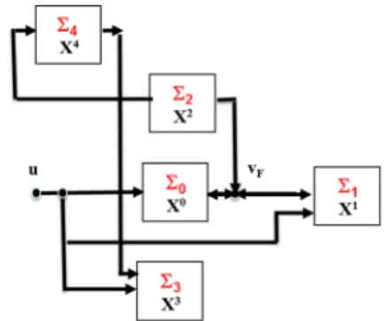
The proof is based on the structural subdivision of the system into 5 subsystems depicted in Figure .1 and defined as follows:
• Σ0 merges the input vertex u, vertex vF and
all the state vertices which are predecessors of
vF and are reachable from u without necessarily
covering vFi.e. the components of Σ0are U∪{vF}∪
(P red(vF)∩ Succ(u) ∩ {vi∈ X, vF∈ V/ ess(U,{vi})})
• Σ1 merges all the state vertices which are successors
of vF and which are not in Σ0, i.e. the components
of Σ1 are ( Succ(vF)\ P red(vF) ) ∪ {vi ∈ X, vF ∈ Vess({u}, {vi})};
• Σ2merges all the state vertices which are predecessors
of vF but not successors of u i.e. the components of
Σ2are P red(vF)\ Succ(u);
• Σ3 merges all the state vertices which are successors
of u but neither predecessors nor successors of vF,
i.e. the components of Σ3are Succ(u)\
(
Succ(vF)∪
P red(vF)
) ;
• Σ4merges all the state vertices which are not
succes-sors of u, not successucces-sors of vF and not predecessors
of vF i.e. the components of Σ4 are X\
(
Succ(u)∪ Succ(vF)∪ P red(vF)
)
. These vertices can be linked to Σ2 and Σ3.
Note that this subdivision is unique and is motivated by the fact that it allows to characterize yF as a flat output
using the controllability and observability characteristics of each subsystem. Indeed, we can make two important remarks on subsystems Σ2and Σ4:
Remark 2. Subsystems Σ2and Σ4are not forced by input
u. So, it is clear that if they don’t involve any cycle
(equivalently to a memorization operator), their state components will go to zero after a finite transient time. Conversely, if they involve at least one cycle, some of their state components will depend, at time k, on its own past value and so on the initial state value. And yet, the initial state of these subsystems cannot be expressed only as a function of the component associated to vFi.e. yF. Indeed,
yFis not sensitive to the state of Σ4and since u is an input
acts on yF, there is no equation linking the present, past
and future values of yFto the state components of Σ2only
without the past and present values of u.
Remark 3. According to Definition 1, it is clear that yF
associated to the vertex vF is a flat output if and only if
• The input can be expressed as a function of the past,
present, future values of yF;
• There exists an integer k0such that for all k≥ k0, all
the state components of all the subsystems are either equal to zero or can be expressed as a function of the past, present, future values of yF.
We are now in position of proving the proposition.
Sufficiency: When condition C2 is satisfied, there is no
cycle in subsystems Σ2and Σ4. In this case and since these
two subsystems are not forced by the input, after a finite time, less or equal to the length of the longest path in these two subsystems, all the state components of these subsystems are equal to zero according to Remark 2. Regarding subsystem Σ0, the generic dimension of its
observability subspace, considering that yF associated to
vF is the output and that u is an unknown input, is equal
to the length of the shortest{u}-{vF} path plus one i.e.
ℓ(u, vF) + 1 (Boukhobza (2010)). Moreover, considering
now that yF associated to vF is the output and that
u is known, the generic dimension of the observability
subspace of the structured system Σ0 is equal to the
longest{u}-{vF} path plus the length of all the disjoint
cycles which are not covered by this path. Nevertheless, when conditions C0, C1 and C2 are valid, the longest
{u}-{vF} path is also the shortest {u}-{vF} and there is no
cycles that are disjoint with these paths in Σ0. Therefore, if
conditions C0, C1 and C2 are satisfied, u can be expressed generically using the present and the past values of yF
associated to vF. Furthermore, all the state components
of Σ0belonging to Vess({u}, {vF}) can also generically be
expressed using the present and the past values of yFsince
they are generically observable considering that yF is the
output (Boukhobza (2010)). Therefore, substituting the input u and all the state vertices of all Vess({u}, {vF}) by
their expression in function of yF, there exists a positive
constant ν such that the linear structured system ΣΛ can
be written as:
ΣΛ: x(k +1) = ˜Ax(k)+ϕ(yF(k), yF(k−1), . . . , yF(k−ν))
(.1) where, as the cycles involve only elements of
Vess({u}, {vF}), the matrix ˜A is an adjacency matrix for
a digraph of a structured system having no cycles. Thus, ˜
A is nilpotent and verifies ˜An = 0. As a result, every state can be expressed as a function of the past, present and future values of yF which is thereby a flat output
according to Remark 3 and Definition 1.
Necessity: If condition C0 is not satisfied, then yF is
not sensitive to u. As a result, the input cannot generically be expressed using the past, present and future values of
yF and yF cannot be a flat output. Condition C0 is then
necessary.
Condition C1 is not applicable to subsystems Σ1, Σ3 or
Σ4. For subsystem Σ0, if conditions C1 is not satisfied
(i.e. if there exist paths u-vF with different lengths
ℓ1 ̸= ℓ2), then the expression of yF at time k, that is
yF(k), will involve at least u(k−ℓ1) and u(k−ℓ2). It is the
same when Σ0involves a cycle. Condition C1 is necessary
for Σ0. Moreover, if condition C2 is not satisfied (i.e.
if there exist cycles which cover the state components which are not in Vess({u}, {vF}), the generic dimension
of the observability subspaces with and without the input knowledge are different. In this case, the input cannot generically be expressed using yF as output. Indeed,
Therefore, condition C2 is necessary for Σ0.
Only condition C2 is applicable to Σ2. If it is not satisfied
i.e. when there is a cycle in Σ2, the expression of yF(k),
will always contain at least a term involving a state component of Σ2, which never equals 0 because of the
cycle, in addition to the u(k− ℓ). So, it is impossible to express the input using only the past, present and future values of yF, and thus yF is not a flat output. Therefore,
condition C2 is necessary for Σ2.
Finally, assume that condition C2 is not satisfied for Σ1, Σ3 or Σ4. In such a case, the values of the state
components of Σ1, Σ3and Σ4depend always on the values
of their initial states which are function of yF. Therefore,
these state components cannot be expressed as a function of exclusively the past, present and future values of yF.