Computationally efficient error-correcting codes and holographic proofs

Computationally Efficient Error-Correcting Codes and

Holographic Proofs

by

Daniel Alan Spielman

B.A., Mathematics and Computer Science

Yale University (1992)

Submitted to the Department of Mathematics

in partial fulfillment of the requirements for the degree of

Doctor of Philosophy

at the

MASSACHUSETTS INSTITUTE OF TECHNOLOGY

June 1995

©

Massachusetts Institute of Technology 1995. All rights reserved.

Signature of Author

,

Department of Mathematics

May 5, 1995

Certified bv

,

Michael Sipser

Professor of Mathematics

Thesis Supervisor

Accepted 1

-Richard Stanley, Chairman

Applied Mathematics Committee

Accepted

by

A

;.1;,SACrHiUStETS INSTilUTE OF TECHNOLOGY

OCT

20

1995

A

_{David Vogan, Chairman}

Departmental Graduate Committee

LIBRARIES

~-Computationally Efficient Error-Correcting Codes and Holographic

Proofs

by

Daniel Alan Spielman

Submitted to the Department of Mathematics on May 5, 1995,

in partial fulfillment of the requirements for the degree of Doctor of Philosophy

Abstract

We present computationally efficient error-correcting codes and holographic proofs. Our error-correcting codes are asymptotically good and can be encoded and decoded in linear time. Our construction of holographic proofs provide, for every proof of any theorem, a slightly larger "holographic" proof whose accuracy can be probabilistically checked by an algorithm that only reads a constant number of the bits of the holographic proof and runs in poly-logarithmic time (such proofs have also been called "transparent proofs" and "prob-abilistically checkable proofs"). We explain how these constructions are related and how improvements of these constructions should result in a strengthening of this relationship.

For every constant r such that 0 < r < 1, we construct an infinite family of systematic

linear block error-correcting codes that have an encoding circuit with a linear number of wires. There is a constant E > 0 and a linear-time decoding algorithm for these codes that maps every word of relative distance at most E from a codeword to that codeword. The encoding circuits have logarithmic depth. The decoding algorithm can be implemented as a circuit with O(n log n) wires and logarithmic depth. These constructions make use of explicit constructions of expander graphs and superconcentrators.

Our constructions of holographic proofs improve on the theorem PCP(log n, 1) = NP,

proved by Arora, Lund, Motwani, Sudan, and Szegedy, by providing, for every E > 0,

constant-query checkable proofs of size O(n 1_{+'). That is, we design a probabilistic} poly-logarithmic time proof checking algorithm that takes two inputs: a theorem candidate and a proof candidate. After reading a constant number of bits from each input, the proof checker decides whether to accept or reject its inputs. For every rigorous proof of length n of any theorem, there is an easily computable holographic proof of that theorem of size O(nl+e) such that, with probability one, the proof checker will accept the holographic proof and an encoding of the theorem. Conversely, if the proof checker accepts a theorem candidate and a proof candidate with probability greater than one-half, then the theorem candidate is close to a unique encoding of a true theorem and the proof candidate constitutes a proof of that theorem.

Thesis Supervisor: Michael Sipser Title: Professor of Mathematics

Credits

Most of the material in this thesis has appeared or will appear in conference proceedings. The material in Chapter 2 is joint work with Michael Sipser and appeared in [SS94]. The material in Chapter 4 appeared in [PS94] and is joint work with Alexander Polishchuk. I would like to thank Alexander Shen for putting me in contact with Polishchuk. The constructions in Chapter 3 will appear in [Spi95]. I thank both Michael Sipser and Alexander Polishchuk for these collaborations.

I would also like to thank the many people who have made useful suggestions to me in this research. Among them, I would especially like to thank Noga Alon, Oded Goldre-ich, Brendan Hassett, Marcos Kiwi, Carsten Lund, Nick Reingold, Michael Sipser, Madhu

Sudan, and Shang-Hua Teng.

My thesis committee consisted of Michel Goemans, Shafi Goldwasser, and Michael Sipser.

Acknowledgments

I have benefited greatly from:

a special grade school education at The Philadelphia School, where we loved to learn without the motivation of grades, and we all cried at the end of the year;

the efforts of inspiring teachers-Carter Fussell, David Harbater, Serge Lang, Richard Davis, Jeffrey Macy, and Richard Beigel; I am fortunate to have encountered so many; educational opportunities and support including the Young Scholars Program at the

University of Pennsylvania, a Research Experience for Undergraduates from the National Science Foundation, a Fellowship from the Hertz Foundation, and three summers at AT&T Bell Laboratories;

the good advice and good listening of my advisor, Michael Sipser; valuable advice, direction, and encouragement from Joan Feigenbaum;

my good friends Meredith Wright, Dave DuTot, Maarten Hoek, Marcos Kiwi, Jon Klein-berg, Shang-Hua and Suzie Teng, and The Crew; true friends are those who take pride in your achievements;

To Mom, Dad, and Darren

Table of Contents

1 Introduction

1.1 Error-correcting codes . . . . 1.2 The purpose of proofs . . . . 1.3 Structure of this thesis . . . . 1.4 An introduction to error-correcting codes

1.4.1 Linear codes . . . .

1.4.2 Asymptotic bounds . . . . 1.5 The complexity of coding . . . .

2 Expander codes

2.1 Introduction to expander graphs . . . . . 2.1.1 The expansion of random graphs . 2.2 Expander codes ...

2.3 A simple example ...

2.3.1 Sequential decoding . . . .

2.3.2 Necessity of Expansion . . . . 2.3.3 Parallel decoding ...

2.4 Explicit constructions of expander graphs 2.4.1 Expander graphs of every size . . . 2.5 Explicit constructions of expander codes .

2.5.1 A generalization

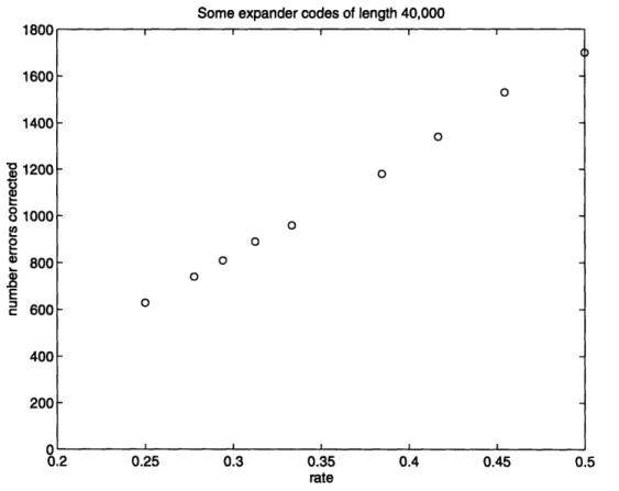
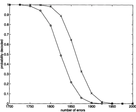
2.6 Notes on implementation and experimenta 2.6.1 Some experiments . . . . .o . . . . ° . . . . . ... ... °. . o o. . .o . . . . ... l results . . . . o

3 Linear-time encodable and decodable error-correcting codes

3.1 Motivating the construction ...

3.4 Explicit Constructions . . . . 3.5 Some thoughts on implementation and future work . 4 Holographic Proofs

4.0.1 Outline of Chapter ...

4.1 Checkable and verifiable codes . . . .

4.2 Bi and Trivariate codes ... 4.2.1 The First Step ...

4.2.2 Resultants... ... ... ... 4.2.3 Presentation checking theorems . . . . 4.2.4 Using Bezout's Theorem . . . . 4.2.5 Sub-presentations and verification . . . .

4.3 A simple holographic proof system . . . . 4.3.1 Choosing a key problem . . . . 4.3.2 Algebraically simple graphs . . . . 4.3.3 Arithmetizing the graph coloring problem 4.3.4 A Holographic Proof ...

4.4 Recursion ...

4.4.1 Encoded inputs ...

4.4.2 Using the Fast Fourier Transform . . . . . 4.5 Efficient proof checkers . . . . 4.6 The coloring problem of Babai, Fortnow, Levin, ai

... o ... ... ° . .e . . . . . . . °. . . . .o . . . .o . .o . .° . . . .o . ... o.. ... ° nd Szegedy . 5 Connections

5.1 Are checkable codes necessary for holographic proofs? . . . .

Bibliography Index 81 83 86 92 94 96 102 103 106 106 113 116 118 125 125 127 131 132 135 137 139 145

CHAPTER 1

Introduction

Mathematical studies of proofs and error-correcting codes played an important role in the development of theoretical computer science. In this dissertation, we develop ideas from theoretical computer science and apply them to the construction of error-correcting codes and proofs. Our goal is to construct error-correcting codes that can be encoded and decoded and proofs that can be verified as efficiently as possible. The error-correcting codes that we build are the first known asymptotically good family of error-correcting codes that can be encoded and decoded in linear time. Our construction of holographic proof systems enables one to transform any rigorous proof system into one whose proofs, while only slightly longer, can be probabilistically checked by the examination of only a constant number of their bits. We conclude by explaining how these constructions of error-correcting codes and holographic proofs are related.

1.1

Error-correcting codes

Error-correcting codes were introduced to deal with a fundamental problem in commu-nication: when a message is sent from one place to another, it is often distorted along the way. An error-correcting code provides a systematic way of adding information to a message so that even if part of the message is corrupted in transmission, the receiver can nevertheless figure out what the sender intended to transmit. Naturally, the probability

that the receiver can recover the original message decreases as the amount of distortion increases. Similarly, the amount of distortion that the receiver can tolerate increases as more redundant information is added to the transmitted message.

In his seminal 1948 paper, A Mathematical Theory of Communication, Shannon [Sha48] proved tight bounds on the amount of redundancy needed to tolerate a given amount of cor-ruption in discrete communication channels. Shannon modeled the communication problem as a situation in which one is trying to send information from a source to a destination over a channel that occasionally becomes corrupted by noise (See Figure 1-1). Shannon described a coding scheme in which the transmitter breaks the original message into pieces, adds some redundant information to each piece to form a codeword, and then sends the codewords. The codewords are chosen so that if the received signal does not differ too much from the sent signal, the receiver will be able to remove the distortion from the received signal, fig-ure out which codeword was sent, and pass the corrected message on to the destination. Shannon defined a notion called the capacity of a channel, which decreases as the amount

INFORMATION

SOURCE TRANSMITTER RECEIVER DESTINATION

NOISE

SOURCE

Figure 1-1: Shannon's schematic of a communication system.

of noise on the channel increases, and demonstrated that it is impossible to reliably send information from the source to the destination at a rate that exceeds the capacity of the channel. Thus, the capacity of the channel determines how much redundant information the transmitter needs to add to each piece of a message. Remarkably, Shannon was able to demonstrate that there is a coding scheme that enables one to reliably send information from the source to the destination at any rate lower than the capacity. Moreover, using such a coding scheme, one can arbitrarily reduce the probability that a message will fail to reach the destination without adding any extra redundant information: one need merely

increase the size of the pieces into which the message is broken.

But, there was a catch. While Shannon demonstrated that it is possible to encode longer and longer pieces of messages, he did not present a efficient means for doing so. Thus, the study of error-correcting codes was born in an attempt to find coding schemes that approx-imate the performance promised by Shannon and to find efficient implementations of these coding schemes. In this thesis, we present the first such coding scheme in which the compu-tational effort needed to encode and decode corrupted codewords is strictly proportional to the length of the codewords. This enables us to arbitrarily reduce the probability of error in communication without decreasing the rate of transmission or increasing the computational work required.

1.2

The purpose of proofs

When we construct error-correcting codes, we are concerned with the transmission of a message, but we ignore its content. In the second part of this thesis, we explore how a receiver can become convinced that a message has a particular content while only reading a small portion of the message.' We formalize this by requiring that the message be a demonstration of some fact, and we consider the content of the message to be the truth of that fact. That is, we treat the message as a proof.

A proof is the means by which one mathematician demonstrates the truth of an assertion to another. Ideally, it should be much easier for the other to become convinced of the truth of the assertion by reading a proof of it than by attempting to derive the veracity of the assertion from scratch. Thus, we view a proof as a labor-saving device: by providing proofs, we provide others with the fruits of our labor, but spare them its pains2_{. By including extra} details and background material, we make our proofs accessible to a broader audience. If we supply sufficient detail, then one almost completely ignorant of mathematics should be able to check the veracity of our claims.

In principle, any mathematical claim and accompanying proof can be expressed using

'Some may try to do this by reading only the introduction of the message, but one cannot be sure that the body will fulfill the promises made in the introduction.

2

We hope that this dissertation achieves this goal.

The purpose of proofs 15 1.2

a few axioms and a simple calculus. The verifier of such a proof need only be able to check that certain simple string operations are performed correctly and that strings have been faithfully copied from one part of the proof to another. By making the proofs slightly longer, it is possible to construct formats for proofs in which the verifier only needs to check that a collection of pre-specified conditions are met, each of which only involves a constant number of bits of the proof. At this point, it seems that we have made the task of the verifier as simple as is conceivably possible. But, by allowing for a little uncertainty, we can make it even simpler.

The complexity class non-deterministic polynomial time, usually called NP, roughly captures the set of facts that have proofs whose size is polynomial in the length of their statement. Similarly, the class non-deterministic exponential time, NEXP, captures the set of facts that have proofs whose size is exponential in the size of the statement of the fact. In their proof that NEXP = MIP, Babai, Fortnow, and Lund [BFL91] demonstrated that it is possible to probabilistically verify the truth of one of these exponentially long proofs while only reading a polynomial number of the bits of the proof. Without reading the whole proof, the verifier cannot be certain that it is true. But, by reading a small portion of the proof, the verifier can be very confident that it is true. That is, the verifier will always accept a correct proof of a true statement; but, if the verifier examines a purported proof of a false statement, then the verifier will reject the purported proof with high probability. The following year, Babai, Fortnow, Levin, and Szegedy [BFLS91] explained how sim-ilar techniques could be combined with some new ideas to construct transparent proofs of any mathematical statement. Their transparent proof of a statement was only slightly longer than the formal proof from which it was derived, but it could be probabilistically verified in time poly-logarithmic (very small) in the size of the proof and the degree of confidence desired. In a related series of papers by Feige, Goldwasser, Lovasz, Safra, and Szegedy [FGL+91], Arora and Safra [AS92b], and Arora, Lund, Motwani, Sudan, and Szegedy [ALM+92], proofs were created that could be probabilistically verified by exam-ining only a constant number of randomly chosen bits of the proof.3 However, the size of

3

These types of proofs have gone by the names transparent proofs, probabilistically checkable proofs, and holographic proofs. We prefer the name holographic proofs, introduced by Levin, because, as in a hologram,

these proofs was at least quadratic in the size of the original proofs.

We construct proofs that combine the advantages of being nearly linear in the size of the original proofs and having verifiers that run in poly-logarithmic time and read only a

constant number of bits of the proof.

Note that we do not advocate the use of such proof systems by practicing mathemati-cians. A mathematician is rarely satisfied with merely knowing that a fact is true. The excitement of mathematics lies in understanding why. While one might obtain such an understanding by reading a holographic proof, it would be much simpler to read a proof written in plain language designed for easy comprehension. We study holographic proofs both because we want to find out how little work one need do to verify a fact and because, in the process of studying this fundamental question, we obtain results that have important implications in other areas.

Among the techniques used to construct and analyze holographic proofs, we would like to point out the importance of those derived from the study of: checkable, self-testable/self-correctable, and random-self-reducible functions [BK89, RS92, BLR90, Rub90, GLR+91, GS92, Lip91, BF90, Sud92, She91]; techniques for reducing our dependence on random-ness [IZ89, Zuc91]; interactive proofs [Bab85, BM88, GMR89, GMR85, BoGKW88, FRS88, LFKN90, Sha90, FL92, LS91, BFL91]; and error-correcting codes [GS92, BW, BFLS91]. Through many of these works one finds a common algebraic thread inspired by the work of Schwartz [Sch80]. The crux of our construction of holographic proofs is a purely algebraic statement-Theorem 4.2.19.

The main application of constructions of holographic proofs has been to prove the hard-ness of finding approximate solutions to certain optimization problems. Notable papers in this direction include [PY91, FGL+91, AS92b, ALM+92, LY94, Zuc93, BGLR93, F94, BS94, ABSS93]. Holographic proofs have also been applied to problems in many areas of complexity theory [CFLS93, CFLS94, Ki192, Ki194, Mic94, KLR+94]. While not properly an application of holographic proof technology, our constructions of error-correcting codes were

each bit of information in a holographic proof is reflected in the entire structure. Some authors reserve the

term probabilistically checkable for proof systems in which the proof checker reads the statement to be proved and use transparent or holographic to describe systems in which the statement of the theorem to be proved

is encoded so that the proof checker only needs to read a constant number of its bits.

The purpose of proofs 17

inspired by these proofs. They were born of an attempt to find an alternative construction of holographic proofs, and we hope that they one day aid in this effort.

1.3

Structure of this thesis

We begin in Section 1.4 with an introduction to the field of error-correcting codes from the perspective of this complexity theorist. In Section 1.5, we describe some of what is known about the complexity of error-correcting codes. The goal of this introduction is to provide a context for the results in Chapters 2 and 3.

Chapters 2 and 3 are devoted to our construction of linear-time encodable and decodable error-correcting codes. In Chapter 2, we describe a construction of codes that can be decoded in linear time, but for which we only know quadratic-time encoding algorithms. These codes can also be decoded in logarithmic time by a linear number of processors. In this chapter, we introduce many of the techniques that we will use in Chapter 3. In particular, we present a relation between expander graphs and error-correcting codes. Along the way, we survey some of what is known about expander graphs. As we feel that these codes might be useful for coding on write-once media, we conclude the chapter by presenting some thoughts on how one might go about implementing these codes.

In Chapter 3, we present our construction of linear-time encodable and decodable error-correcting codes. These codes can also be encoded and decoded in logarithmic time with a linear number of processors. We call these codes superconcentrator codes because their encoding circuits bear a strong resemblance to superconcentrators. As part of our construc-tion, we develop a type of code that we call an error-reducing code. An error-reducing code enables one to quickly remove most of the errors from a corrupted codeword, but it need not allow full error-correction. We construct superconcentrator codes by carefully piecing together appropriately chosen error-reducing codes. Again, we conclude this chapter with some thoughts on how one might implement these codes and on how they could be improved. Chapter 4 is devoted to our construction of nearly linear size holographic proofs. This Chapter is somewhat more involved than Chapters 2 and 3, but it should be intelligible to the reader with a reasonable background in theoretical computer science. We begin by

describing holographic proofs and by defining some of the types of error-correcting codes that they are related to. A potentially useful type of error-correcting code derived from holographic proofs is a checkable code. Checkable codes have associated randomized algo-rithms that, after examining only a constant number of randomly chosen bits of a received word, can make a good estimation of the probability that a decoder will successfully decode the word. One could use such an algorithm to decide whether to request the retransmis-sion of a word even before the decoder has worked on it. In Section 4.2, we develop the algebraic machinery that we will need to construct our holographic proofs. We show that certain polynomial codes are somewhat checkable and verifiable. These codes are used in Section 4.3 to construct our basic holographic proof system. We apply this system to itself recursively to construct our efficient holographic proofs. In the final sections, we present a few variations of our construction, each more powerful, but more complicated, than the previous.

In the last chapter of this thesis, we explain some of the connections between our con-structions of error-correcting codes and holographic proofs. We explain the similarities between expander codes and the checkable codes derived from holographic proofs. We also discuss whether checkable codes are a necessary component of holographic proofs. Our conclusion is that the problems of constructing more efficient checkable codes, holographic proofs, and expander codes are strongly linked, and could even have the same solution.

1.4

An introduction to error-correcting codes

The purpose of this section is to provide the reader with a convenient reference for the basic definitions from the field of error-correcting codes that we will use in this thesis. Those who understand the phrase "asymptotically good family of systematic linear error-correcting codes" can probably skip this section.

Intuitively, a good error-correcting code is a large set of words such that each pair differs in many places. Let E be a finite alphabet with q letters. A code of length n over E is a subset of En. Throughout most of Chapters 2 and 3, we will discuss codes over the alphabet

{0,

should be assumed to be binary.

Two important parameters of a code are its rate and minimum distance. The rate of a code C is (logq Cl )/n. The rate indicates how much information is contained, on average, in each code symbol. The minimum distance of a code C is

min d(x, y),

X,yEC

where d(x, y) is the Hamming-distance between two words (i.e., the number of places in which they differ). We will usually talk about the relative minimum distance of a code,

d(x, y)/n.

Since we are interested in the asymptotic performance of codes, we define a family of

error-correcting codes to be an infinite sequence of error-correcting codes that contains at

most one code of any length. If {Ci} is a family of error-correcting codes such that, for all

i, the rate of Ci is greater than r, then we say that the family has rate at least r. Similarly,

if the relative minimum distance of each code in the family is at least 6, then we say that the relative minimum distance of the family is at least 6. An infinite family of codes over a fixed alphabet is called asymptotically good if there exist positive constants r and 6 such that the family has rate and relative minimum distance at least r and 6 respectively.4 A central problem of coding theory has been to find explicit constructions of asymptotically

good families of error-correcting codes with as large rate and relative minimum distance as possible.

The preceding definitions are standard. We will now make some less standard definitions that will help us discuss the complexity of encoding and decoding error-correcting codes.

An encoding function for a code C of rate r is a bijection

f: E'"

C.

We say that an encoding function is systematic if there exist indices il,..., i,, such that for

all

)

Frn,

(x1,... iX,, ,) (= ( ,),,.f(Mi,,).

That is, the message is embedded in the codeword. If a code has a systematic encoding function, then we say that the code is systematic. We can think of a systematic code as being divided into rn "message symbols" and (1 - r)n "check symbols". The check symbols are uniquely determined by the message symbols, and we can view the message symbols as containing the information content of the codeword (in a binary code, we will call these message bits and check bits).

An error-correcting function for a code C is a function

g : " -- C U

{?}

such that g(x) = x, for all x E C. We say that an error-correcting function for C can correct m errors if for all x E C and all y E E" such that d(x, y) < m, we have g(y) = x. We allow

an error-correcting function to return the value "?" so that it can describe the output of an algorithm that could not find an element of C close to its input. We use the verb decode loosely to indicate the process of correcting a constant fraction of errors. When we say a

"decoding algorithm", we mean an algorithm that can correct some constant fraction of errors. From the perspective of a complexity theorist, the fraction of errors that can be efficiently corrected in a family of error-correcting codes is much more interesting than the

An introduction to error-correcting codes 21 1.4

actual minimum distance of those codes.

1.4.1

Linear codes

The codes that we construct will be linear codes. A linear code is a code whose alphabet is a field and whose codewords form a vector space over this field. There are two natural ways to represent a linear code: either by listing a basis of the space and defining the code to be all linear combinations of those basis vectors, or by listing a basis of the dual space. A matrix whose rows are a basis of the dual space is called a check matrix of the code.

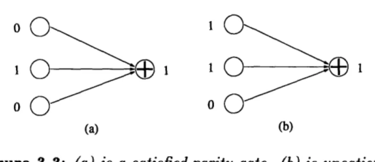
In a binary code, each check bit is just a sum modulo 2 of a subset of the message bits. Some elementary facts that we will use about linear binary codes are:

* The zero vector is always a codeword.

* They are systematic. To see this, row reduce the (1 - r)n x n check matrix until it

contains (1 - r)n columns that contain exactly one 1. These columns correspond to

the check bits, and the remaining rn columns correspond to the message bits. Observe that row-reducing the check matrix does not change the code that it defines. It is now clear that for any setting of the message bits, there is a unique setting of the check bits so that the resulting vector is orthogonal5 to every row in the row-reduced check matrix.

* They can be encoded using O(n2) work: there is a rn x (1 - r)n matrix such that

the check bits can be computed from the message bits by multiplying the vector of

rn message bits by this matrix. (This is the matrix that appears in the columns

corresponding to the message bits described in the previous item.)

* The minimum distance of a linear code is equal to the minimum weight of a non-zero codeword (the weight of a codeword w is d(O, w); note that d(v, w) = d(O, w - v)).

5_{We say that two vectors are orthogonal if their inner product is zero. Over a finite field, this loses its}

1.4.2 Asymptotic bounds

Good linear codes are easy to construct. A randomly chosen parity check matrix defines a

good code with exponentially high probability.

Theorem 1.4.1 Let vl,...,van be vectors chosen uniformly at random from GF(2)n. Let

C be the code consisting of the length n vectors over GF(2) that are orthogonal to all of vl,..., va,. C has rate at least 1 - a. With high probability, C has relative minimum distance at least E, for E < 1/2 and a > H(E), where H(.) is the binary entropy function

(i.e. H(x)=

Proof: The probability that any non-zero word is orthogonal to each of vl,..., v,an is 2-n". Thus, the probability that some non-zero vector of weight at most En is orthogonal to each of vl,..., van is at most SE, (f)2-o". One can use Stirling's formula to show that, for fixed e, log2 (n) = nH(E)+ O(log n). Thus, the sum approaches zero if a > H(e). U

Codes with rate r and minimum relative distance e for r > 1 - H(E) are said to meet the

Gilbert- Varshamov bound. While these random linear codes may be encoded using quadratic

work, we know of no efficient algorithm for decoding them.

An easy upper bound on the performance of a code is the sphere-packing bound:

Theorem 1.4.2 Let Cn be an infinite sequence of codes with relative minimum distance at least 6. Then

limsup rate(Cn) _ 1 - H(b/2). n-0oo

Proof: If the code has minimum distance 6n, then there are disjoint balls of radius 1n/2

around each codeword. These balls account for at least 2r n _{(n/2) words; but, there are only}

2" words of length n. U

Better upper bounds than the sphere-packing bound are known. The Elias bound, which held the record for a long time, has a fairly simple proof.

Theorem 1.4.3 [Elias] Let C, be an infinite sequence of codes with relative minimum distance at least 6. Then

lim sup rate(Cn) < 1

-

H

(1

11-2

n-+o 2 2

An introduction to error-correcting codes 23

Even better, but much more complicated to prove, is the McEliece-Rodemich-Rumsey-Welch upper bound:

Theorem 1.4.4 [McEliece-Rodemich-Rumsey-Welch] Let C, be an infinite sequence of codes with relative minimum distance at least 6. Then

lim sup rate(Cn) H - - (1- ₎

n be foo in [MS77]. Proofs of both of these can be found in [MS77].

The complexity of coding 25

1.5

The complexity of coding

Many of the foundations for the analysis of the complexity of algorithms were laid by Shan-non in his 1949 paper The synthesis of two-terminal switching circuits [Sha49]. Suggestions for how to analyze the complexity issues special to error-correcting codes appeared in the work of Savage [Sav69, Sav71] and Bassalygo, Zyablov, and Pinsker [BZP77]. For more gen-eral studies of the complexity of algorithms, we point the reader to [AHU74] and [CLR90]. From our perspective, the relevant questions are: how hard is it to encode a family of error-correcting codes, and how much time does it take to correct a constant fraction of errors? We are not as interested in the minimum distance of a code as we are in the number of errors that we can efficiently correct. We measure encoding and decoding efficiency by the time of a RAM algorithm or the size and depth of a boolean circuit that performs the operations. Bassalygo, Zyablov, and Pinsker point out that we should also examine the complexity of building the encoding and decoding programs or circuits. While we do not discuss this in detail, it will be clear that there are efficient polynomial-time algorithms for constructing our encoding and decoding programs and circuits.

Initially, the only algorithms known for decoding error-correcting codes were exponential in complexity: enumerate all codewords and select one closest to the received word. For linear codes, one could do slightly better by computing which parity checks were violated and searching for the smallest pattern of errors that would violate exactly that set of parity checks. There were numerous improvements on these approaches. We will not attempt to survey the accomplishments of coding theory; we will just mention the most efficient coding algorithms known prior to our work: Using efficient implementations of the Finite Fourier Transform, Justesen [Jus76] and Sarwate [Sar77] have shown that certain Reed-Solomon and Goppa codes can be encoded in O(nlog n) time and decoded in time 0 (nlog2_n). While these codes are not necessarily asymptotically good, one can compose them with good codes to obtain asymptotically good codes with similar encoding and decoding times. Moreover, these algorithms are easily parallelized.

Codes that have more efficient algorithms for one of these operations have suffered in the other. Gelfand, Dobrushin, and Pinsker [GDP73] presented randomized constructions

of asymptotically good codes that could be encoded in linear time. However, they did not suggest algorithms for decoding their codes, and we suspect that a polynomial-time algorithm would be difficult to find.

Zyablov and Pinsker [ZP76] showed that it is possible to decode Gallager's randomly chosen low-density parity-check codes [Gal63] in logarithmic time with a linear number of processors. These codes are essentially the same as those we present in Section 2.3. We are not aware of any algorithm for encoding these codes that uses less than O(n2_{) work.} Kuznetsov [Kuz73] used these codes to construct fault-tolerant memories. Pippenger has pointed out that Kuznetsov's proof of the correctness of these memories can serve as a proof of correctness of the parallel decoding algorithm that we present in Section 2.3.3. By analyzing these codes in terms of the expansion properties of the graphs by which they are defined, we are able to provide a much simpler proof of the correctness of the parallel decoding algorithm, prove for the first time the correctness of the natural sequential decoding algorithm presented in Section 2.3.1, and obtain the first explicit constructions of asymptotically good low-density parity-check codes.

CHAPTER 2

Expander codes

In this chapter, we explain a way of using expander graphs to construct asymptotically good linear error-correcting codes. These codes can be decoded in linear sequential time or parallel logarithmic time with a linear number of processors. The best encoding algorithms that we know for these codes are the O(n2 ) time algorithms that can be used for all linear codes. These codes fall into the category of low-density parity-check codes introduced by Gallager [Gal63]. The construction that we present in Section 2.5 is the first known explicit construction of an asymptotically good family of low-density codes.

We begin by explaining what expander graphs are and prove that good expander graphs exist. In Section 2.2, we define expander codes precisely and prove that they can be asymp-totically good. In Section 2.3, we show how error-correcting codes derived from very good expander graphs can be efficiently decoded. The construction that we present in this section is similar to Gallager's construction. In Section 2.3.1, we provide the first proof of correct-ness for the natural sequential algorithm for decoding these codes. In Section 2.3.2, we demonstrate that this algorithm only works on codes derived from expander graphs. Thus, Gallager's codes work precisely when the graphs from which they are derived are expanders. Unfortunately, we are not aware of deterministic constructions of expander graphs with the level of expansion needed for this first construction.

graphs. We use these constructions in Section 2.5 to produce explicit constructions of expander codes that can be decoded efficiently.

We conclude this chapter with a discussion of how one might want to implement these codes and a presentation of the results of experiments which demonstrate the good perfor-mance of these codes.

2.1

Introduction to expander graphs

An expander graph is a graph in which every set of vertices has a large number of neighbors. It is a perhaps surprising but nonetheless well known fact that expander graphs that expand by a constant factor, but which have only a linear number of edges, do exist. In fact, a simple randomized process will produce such a graph.

Let G = (V, E) be a graph on n vertices. To describe the expansion properties of G, we

say every set of size at most m expands by a factor of c if, for all sets S C V,

ISI < m l{y 3x E S such that (x, y) E}I> c S .E

One can show that for all

e

random d-regular graph will probably expand by a factor of d - 1 -

E

In our constructions, we will make use of unbalanced bipartite expander graphs. That is, the vertices of the graph will be divided into two sets such that there are no edges between vertices in the same set. We will call such a graph (d, c)-regular if all the nodes in one set have degree d and all the nodes in the other have degree c. By counting edges, we find that the number of d-regular vertices must differ from the number of c-regular vertices by a factor of c/d. We will only consider the expansion of sets of vertices contained within one

side of the graph. In Section 2.1.1, we will show that if c > d and one chooses a (d, c)-regular graph at random, then it will have expansion approaching d - 1 from the large side to the

small side and expansion approaching c - 1 from the small side to the large side.

We wish to point out that Alon, Bruck, Naor, Naor, and Roth [ABN+92] used expander graphs in a different way to construct asymptotically good families of error-correcting codes that lie above the Zyablov bound [MS77]. Also, Alon and Roichman [AR94] use error-correcting codes to construct expander graphs.

2.1.1 The expansion of random graphs

In this section, we will prove upper and lower bounds on the expansion factors achieved by random graphs that become tight as the degrees of the graphs become large.

We first prove a simple upper bound on the expansion any graph can achieve.

Theorem 2.1.1 Let B be a bipartite graph between n d-regular vertices and An c-regular

vertices. For all 0 < a < 1, there exists a set of an d-regular vertices with at most

d

n- (1 - (1 - a)c) + 0(1) neighbors. c

Proof: Choose a set X of an d-regular vertices uniformly at random. Now, consider the probability that a given c-regular vertex is not a neighbor of the set of d-regular ver-tices. Each neighbor of the c-regular vertex is in the set X with probability a. Thus, the probability that the c-regular vertex is not a neighbor of X is

c-1

n - an -

i

II

n-i

'

i=0

which tends to (1 - a)c as n grows large. This implies that the expected number of non-neighbors tends to nr(1 - a)c.

This simple upper bound becomes tight as d grows large.

How to choose a random (d, c)-regular graph: To choose a random (d, c)-regular

bipartite graph, we first choose a random matching between dn "left" nodes and dn "right" nodes. We collapse consecutive sets of d left nodes to form the n d-regular vertices, and we

collapse consecutive sets of c right nodes to form the 4n c-regular vertices. It is possible that this graph will have multiedges that should be thrown away, but this does not hurt the lower bound on the expansion of this graph that we will prove.

To make our language consistent with the rest of this chapter, we will call the d-regular vertices "variables" and the c-regular vertices "constraints".

Theorem 2.1.2 Let B be a randomly chosen (d, c)-regular bipartite graph between n variables and !n constraints. Then, for all 0 < a < 1, with exponentially high probability all sets of an variables in B have at least

n (C(1 - (1 - a)c) - 2daH(a)/ log2e)

neighbors, where H(-) is the binary entropy function.

Proof: First, we fix a set of an variables, V, and estimate the probability that V's set of neighbors is small. The probability that a given constraint is a neighbor of V is at least

1 - (1 - a)c. Thus, the expected number of neighbors of V is at least n (1 - (1 - a)c).

Noga Alon suggested that we form a martingale (See [AS92a]) to bound the probability that the size of the set of neighbors deviates from this expectation.

Each node in V will have d outgoing edges. We will consider the process in which the destinations of these edges are revealed one at a time. We will let Xi be the random variable equal to the expected size of the set of neighbors of V given that the first i edges leaving V have been revealed. X1,...,Xdan form a martingale such that

Ixi+

-

Xi <• 1,

for all 0 < i < dan. Thus, by Azuma's Inequality (See [AS92a]),

Prob[E[Xdon] - Xdan > AVd-] < e- 2/2.

But, E[Xd,n] is just the expected number of neighbors of V. Moreover, Xdan is the expected size of the set of neighbors of V given that all edges leaving V have been revealed, which is

exactly the size of the set of neighbors of V.

Since there are only

(n)

an

By Stirling's formula, this holds for large n if A satisfies

nH(a)/log2e < A2/2 F2nH(a)/log2e <

A.

In general, if a graph has good expansion on a certain size set, then it will have similar expansion on smaller sets. However, this is not always true. What we can say is that the probability that sets of a certain size have a given expansion factor is a unimodal function. Theorem 2.1.2 shows that the probability of failure is exponentially small for large sets. However, for sets of constant size the probability of failure will be only polynomially small. One can probably show that whenever the probability that large sets have a certain expansion factor is exponentially small, all smaller sets will have the same expansion factor with high probability.

2.2

Expander codes

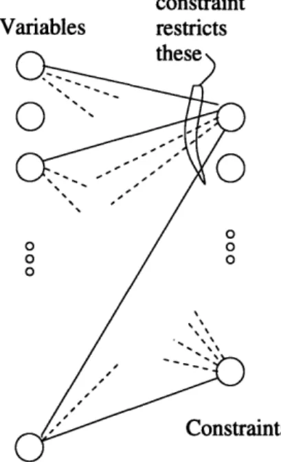
To build an expander code, we begin with an unbalanced bipartite expander graph. Say that the graph is (d, c)-regular between sets of vertices of size n and An, and that c > d. We will identify each of the n nodes on the large side of the graph with one of the bits in a code of length n. We will usually refer to these n bits as variables. Each of the dn vertices on the small side of the graph will be associated with a constraint. Each constraint will restrict only those variables that are neighbors of the vertex identified with the constraint (See Figure 2-1). These will be called the "variables in the constraint". A constraint will require that the variables it restricts form a codeword in some linear code of length c. Because each constraint we impose upon the variables is linear, the expander codes we construct will be linear as well. It is convenient to let all the constraints be the same.

Expander codes 31

constraint Variables restricts

aints

Figure 2-1: A constraint restricts the variables that are its neighbors.

Definition 2.2.1 Let B be a bipartite graph between n variables and In constraints that is d-regular on the variables and c-regular on the constraints. Let 8 be a code of block-length c.

A constraint is satisfied by a setting of the variables if the variables in that constraint form a

codeword of S. The expander code C(B, S) consists of the settings of the variables that satisfy every constraint.

If the expander graph is a sufficiently good expander and if the constraints are identified with sufficiently good codes, then the resulting expander code will be a good code.

Theorem 2.2.2 Let B be a bipartite graph between n variables and in constraints that is d-regular on the variables and c-regular on the constraints. Let 8 be a code of block-length c, rate r, and relative minimum distance E. If B expands by a factor of more than 4 on all setscE

of size at most an, then C(B, S) has rate at least dr - (d - 1) and relative minimum distance

at least a.

Proof: To obtain the bound on the rate of the code, we will count the number of linear restrictions imposed by the constraints. Each constraint induces (1 - r)c linear restrictions.

Thus, there are a total of

n-(1 - r)c = dn(1 - r)

linear restrictions, which implies that there are at least n(dr - (d - 1)) degrees of freedom. To prove the bound on the minimum distance, we will show that there can be no non-zero codeword of weight less than an. Let w be a non-non-zero word of weight at most an and let V be the set of variables that are 1 in this word. There are dIVI edges leaving the variables in V. The expansion property of the graph implies that these edges will enter more than d4

VI

Remark 2.2.3 A construction of codes defined by identifying the nodes on one side of a

bipartite graph with the bits of the code and identifying the nodes on the other side with subcodes first appeared in the work of Tanner [Tan81]. Following Gallager's lead, Tanner analyzed the performance of his codes by examining the girth of the bipartite graph. Margulis [Mar73] also used high-girth graphs to construct error-correcting codes. Unfortunately, it seems that analysis resting on high-girth is insufficient to demonstrate that families of codes are asymptotically good.

2.3

A simple example

A simple example of expander codes is obtained by letting B be a graph with expansion greater than A on sets of size at most an, and letting S be the code consisting of words of even weight. The parity-check matrix of the resulting code, C(B, S), is just the adjacency matrix of B. The code S has rate - and minimum relative distance 2, so C(B, S) has rate 1 - d and minimum distance at least an.

To obtain a code that we can decode efficiently, we will need even greater expansion. With greater expansion, small sets of corrupt variables will induce non-codewords in many constraints. By examining these "unsatisfied" constraints, we will be able to determine which variables are corrupted. In Sections 2.3.1 and 2.3.3, we will explain how to decode these simple expander codes.

A simple example 33 2.3

Unfortunately, we do not know of explicit constructions of expander graphs with ex-pansion greater than 4. Thus, in order to construct these simple codes, we must use the randomized construction of expanders explained in Section 2.1.

2.3.1 Sequential decoding

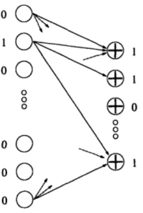
There is a natural algorithm for decoding these simple expander codes. We say that a constraint is "satisfied" by a word w if the sum of the values that w assigns to the variables in the constraint is even; otherwise, we call the constraint "unsatisfied". Consider what happens when we flip' a variable that is in more unsatisfied than satisfied constraints. The unsatisfied constraints containing the variable become satisfied, and vice versa. Thus, we have decreased the total number of unsatisfied constraints. The idea behind the sequential decoding algorithm is to keep doing this until no unsatisfied constraints remain, in which case we have a codeword. Theorem 2.3.1 says that if the graph used to define the code is a good expander and if not too many variables of a codeword are corrupted, then this algorithm will succeed.

Sequential expander code decoding algorithm:

* If there is a variable that is in more unsatisfied than satisfied constraints, then flip the value of that variable.

* Repeat until no such variables remain.

It is easy to implement this algorithm so that it runs in linear time (assuming that pointer references have unit cost). In Figure 2-2, we present one such way of implementing this algorithm. We assume that the graph has been provided to the algorithm as a graph of pointers in which each constraint points to the variables it contains, and each variable points to the constraints in which it appears. The implementation runs in two phases: a set-up phase that requires linear time, and then a loop that takes constant time per iteration. During the set-up phase, the variables are partitioned into lists by the number of unsatisfied constraints in which they appear. During normal iteration of the loop, a variable

1

Set-up phase

For each constraint, compute the parity of the sum of the variables it contains. (The algorithm should have a list of the constraints.)

Initialize lists Lo, ... , Ld.

For each variable, count the number of unsatisfied constraints in which it appears. If this number is i, then put the variable in list Li.

Loop

Until lists Lrd/2,... , Ld are empty do:

Find the greatest i such that Li is not empty Choose a variable v from list Li

Flip the value of variable v

For each constraint c that contains variable v Update the status of constraint c

For each variable w in constraint c

Recompute the number of unsatisfied constraints in which w appears. Move it to the appropriate list.

If all variables are in list Lo, the output the values of the variables. Otherwise, report "failed to decode".

Figure 2-2: An implementation of sequential expander code decoding algorithm.

that appears in the greatest number of unsatisfied constraints is flipped; the status of each constraint that contains that variable is updated; and each variable that appears in each of those constraints is moved to the list that reflects its new number of unsatisfied constraints. If, at some point, there is no variable in more unsatisfied than satisfied constraints, the implementation leaves the loop and checks whether it has successfully decoded its input. If all the variables are in the list Lo, then there are no unsatisfied constraints and the implementation will output a codeword. We will show that the loop is executed at most a linear number of times.

Theorem 2.3.1 Let B be a bipartite graph between n variables of degree d and 4n constraints

of degree c such that all sets X of at most an variables have at least (Q + E)djXI neighbors, for some E > 0. Let C(B) be the code consisting of those settings of the variables that cause every constraint to have parity zero. Then the sequential decoding algorithm will correct up to an

a/2 fraction of errors while executing the decoding loop at most don/2 times. Moreover, the

algorithm runs in linear time on all inputs, regardless of whether or not B is a good expander. A simple example 35 2.3

Proof: _{We will say that the decoding algorithm is in state (v, u) if v variables are}

corrupted and u constraints are unsatisfied. We view u as a potential associated with v. Our goal is to demonstrate that the potential will eventually reach zero. To do this, we will show that if the decoding algorithm begins with a word of weight at most an/2, then, at every step, there will be some variable with more unsatisfied neighbors than satisfied neighbors.

First, we consider what happens when the algorithm is in a state (v, u) with v < an. Let s be the number of satisfied neighbors of the corrupted variables. By the expansion of the graph, we know that

u+s (s3 + C dv.

Because each satisfied neighbor of the corrupted variables must share at least two edges with the corrupted variables, and each unsatisfied neighbor must have at least one, we know that

dv 2 u + 2s.

By combining these two inequalities, we obtain

S< -- -E) dv and u > - + 2E dv. (2.1)

Since each unsatisfied constraint must share at least one edge with a corrupted variable, and since there are only dv edges leaving the corrupted variables, we see that at least a (1 + 2E)

fraction of the edges leaving the corrupted variables must enter unsatisfied constraints. This implies that there must be some corrupted variable such that a (I + 2E) fraction of its

neighbors are unsatisfied. Of course, this does not mean that the decoding algorithm will decide to flip a corrupted variable.

However, it does mean that the only way that the algorithm could fail to decode is if it flips so many uncorrupt variables that v becomes greater than an. Assume by way of contradiction that this happens. Then there must be some time at which v equals an. At this time, equation (2.1) tells us that u > 4an. This leads to a contradiction because u is initially at most Aan and can only decrease during the execution of the algorithm.

_{2U~ ~L W1VLJU~~IU}

_LIIB

_{UL ~UU~s}

_Lur~urssr

This would imply that the algorithm was in a state (an, u), where u < 4an, because u

was initially at most -an. But, this would contradict the analysis above.

To see that the implementation of the sequential decoding algorithm runs in linear time, first observe that the degree of every variable and constraint is constant; so, the set-up phase requires linear time. Moreover, every time a variable is flipped by the algorithm, the number of unsatisfied constraints decreases. Thus, the loop cannot be executed a number of times greater than the number of constraints. Because the degree of each variable and constraint is constant, each iteration requires only constant time. U

We note that it is possible to improve the constants in this analysis by taking into account the fact that after each decoding step, the number of corrupted variables actually decreases by at least 2- - d.

2.3.2 Necessity of Expansion

We will now show that the sequential decoding algorithm works only if the graph B is an expander graph.

Theorem 2.3.2 Let B be a bipartite graph between n variables of degree d and 4n constraints

of degree c such that the sequential expander code decoding algorithm successfully decodes all sets of at most an errors in the code C(B). Then, all sets of an variables must have at least

an 1+ 23 d-1j

_2c

neighbors in B.

Proof: _{We will first deal with the case in which d is even. In this case, every time a}

variable is flipped, the number of unsatisfied constraints decreases by at least 2. Consider the performance of the decoding algorithm on a word of weight an. Because the algorithm stops when the number of unsatisfied constraints reaches zero, the algorithm must decrease the number of unsatisfied constraints by at least 2an as it corrects the an corrupted variables. Thus, every word of weight an must cause at least 2an constraints to be unsatisfied, so

A simple example 37

every set of an variables must have at least 2an neighbors. Because we assume that c > d,

2d-1

2>1+ 2c

3+ 3+ d-l12c

and we are done with the case in which d is even.

When d is odd, we can only guarantee that the number of unsatisfied constraints will decrease by 1 at each iteration. This means that every set of an variables must induce at least an unsatisfied constraints. Alone, this is insufficient to demonstrate expansion by a factor greater than 1. However, let us consider what must happen for the algorithm to be in a state in which an variables are corrupted, but there is no variable that the decoding algorithm can flip that will cause the number of unsatisfied constraints to decrease by more than 1. This means that each corrupted variable has at least d2 of its edges in satisfied constraints. Because each satisfied constraint can have at most c incoming edges, this implies that there must be at least and satisfied neighbors of the an variables. Thus, the

set of an variables must have at least an(1 + d-) neighbors.

On the other hand, if the algorithm decreases the number of unsatisfied constraints by more than 1, then it must decrease the number by at least 3. For some word of weight an,

assume that the algorithm flips flan variables before it flips a variable that decreases the number of unsatisfied constraints by only 1. The original set of an variables must have had

at least

3/an

m)an

neighbors. On the other hand, once the algorithm flips a variable that causes the number of unsatisfied constraints to decrease by 1, we can apply the bound of the previous paragraph to see that the variables must have at least

(1 - )an1 + d

neighbors. We note that this bound is strictly decreasing in

f,

2.3

when p is chosen so that

3pan+(1l- )an = (1+ ) (1- O)an

1+20 = (1-0)(1 +-) (3+d-) =d-1

d-1

d-+

3+ _2c

When we plug 3 back in, we find that the set of an variables must have at least

d-1

d-1

an

(3

2C

2C

~=

= an 1+

₃

₊

d-1

₂

_-l-2c

2.3.3

Parallel decoding

The sequential decoding algorithm has a natural parallel analogue: in parallel, flip each variable that appears in more unsatisfied than satisfied constraints. We will see that this algorithm can also correct a constant fraction of errors if the code is derived from a suffi-ciently good expander graph.

Parallel expander code decoding algorithm:

* In parallel, flip each variable that is in more unsatisfied than satisfied constraints.

* Repeat until no such variables remain.

Theorem 2.3.3 Let B be a bipartite graph between n variables of degree d and dn constraints of degree c such that all sets X of at most

aon

+E)dlXI

code decoding algorithm will correct any

a

2(14)

A simple example 39

Proof: Assume that the algorithm is presented with a word of weight at most an, where

a < 0(1+4,) We will refer to the variables that are 1 as the corrupted variables, and we

will let S denote this set of variables. We will show that after one decoding round, the algorithm will produce a word that has at most (1 - 2E)an corrupted variables.

To this end, we will examine the sizes of F, the set of corrupted variables that fail to flip in one decoding round, and C, the set of variables that were originally uncorrupt, but which become corrupt after one decoding round. After one decoding round, the set of corrupted variables will be CU F. Define v ISI, and set q, y, and 6 so that IF| = qv, ICI = yv, and

IN(S)l = bdv. By expansion, 6 >

+

e.

+ <

_{1 +}

We will first show that

S<

We can bound the number of neighbors of S by observing that each variable in F must share at least half of its neighbors with other corrupted variables. Thus, each variable in

F can account for at most -d neighbors, and, of course, each variable in S \ F can account

for most d neighbors, which implies

6dv -d v + d(1 -q)v

4

S

4-46.

We now show that

I+E

Assume by way of contradiction that this is false. Let C' be a subset of C of size -$+c)v.

Each variable in C' must have at least 4 edges that land in constraints that are neighbors of S. Thus, the total number of neighbors of C' U S is at most

d C' + Sdv. 2