HAL Id: hal-01369906
https://hal.inria.fr/hal-01369906
Submitted on 13 Mar 2017
HAL is a multi-disciplinary open access
archive for the deposit and dissemination of
sci-entific research documents, whether they are
pub-lished or not. The documents may come from
teaching and research institutions in France or
abroad, or from public or private research centers.
L’archive ouverte pluridisciplinaire HAL, est
destinée au dépôt et à la diffusion de documents
scientifiques de niveau recherche, publiés ou non,
émanant des établissements d’enseignement et de
recherche français ou étrangers, des laboratoires
publics ou privés.
Sensing Image Classification
Emmanuel Maggiori, Yuliya Tarabalka, Guillaume Charpiat, Pierre Alliez
To cite this version:
Emmanuel Maggiori, Yuliya Tarabalka, Guillaume Charpiat, Pierre Alliez.
Convolutional
Neu-ral Networks for Large-Scale Remote Sensing Image Classification.
IEEE Transactions on
Geo-science and Remote Sensing, Institute of Electrical and Electronics Engineers, 2017, 55, pp.645-657.
�10.1109/tgrs.2016.2612821�. �hal-01369906�
Convolutional Neural Networks for Large-Scale
Remote Sensing Image Classification
Emmanuel Maggiori, Student member, IEEE, Yuliya Tarabalka, Member, IEEE,
Guillaume Charpiat, and Pierre Alliez
Abstract—We propose an end-to-end framework for the dense, pixelwise classification of satellite imagery with convolutional neural networks (CNNs). In our framework, CNNs are directly trained to produce classification maps out of the input images. We first devise a fully convolutional architecture and demonstrate its relevance to the dense classification problem. We then address the issue of imperfect training data through a two-step training approach: CNNs are first initialized by using a large amount of possibly inaccurate reference data, then refined on a small amount of accurately labeled data. To complete our framework we design a multi-scale neuron module that alleviates the common trade-off between recognition and precise localization. A series of experiments show that our networks take into account a large amount of context to provide fine-grained classification maps.
Index Terms—Classification, satellite images, convolutional neural networks, deep learning.
I. INTRODUCTION
T
HE ANALYSIS of remote sensing images is of paramount importance in many practical applications, such as precision agriculture and urban planning. Recent technological developments have significantly increased the amount of available satellite imagery. Notably, the constel-lation of Pl´eiades satellites produces high spatial resolution images that cover the whole Earth in less than a day. The large-scale nature of these datasets introduces new challenges in image analysis. In this paper we address the problem of pixelwise classification of satellite imagery.There is a vast literature on classification approaches that take into account the spectrum of every individual pixel to assign it to a certain class. Alternatively, more advanced techniques combine information from a few neighboring pixels to enhance the classifiers’ performance, often referred to as spectral-spatial classification. These approaches rely on the separability of the different classes based on the spectrum of a single pixel or of some neighboring pixels. In a large-scale setting, however, these approaches are not effective. On the one hand, current large-scale satellite imagery does not use high spectral resolution sensors, making it difficult to distinguish object classes solely by their spectrum. On the other hand, due to the large spatial extent covered by the datasets, classes have a considerable internal variability, which further challenges the class separability when simply E. Maggiori, Y. Tarabalka and P. Alliez are with Univerist´e Cˆote d’Azur, TITANE team, Inria, 2004 Route des Lucioles, BP93 06902 Sophia Antipolis Cedex, France. E-mail: [email protected].
G. Charpiat is with Tao team, Inria Saclay–ˆIle-de-France, LRI, Bˆat. 660, Universit Paris-Sud, 91405 Orsay Cedex, France.
Manuscript received ...; revised ...
observing the spectral signatures of a restricted neighborhood. We argue that a more thorough understanding of the context such as, e.g., the shape of objects, is required to aid the classification process.
Convolutional neural networks (CNNs) [1] are therefore gaining attention, due to their capability to automatically discover relevant contextual features in image categorization problems. CNNs consist of a stack of learned convolution filters that extract hierarchical contextual image features, and are a popular form of deep learning networks. They are already outperforming other approaches in various domains such as digit recognition [2] and natural image categorization [3].
Our goal is to devise an end-to-end framework to clas-sify satellite imagery with CNNs. The context of large-scale satellite image classification introduces certain challenges that we must address in order to turn CNNs into a relevant classification tool. Notably, we must (1) design a specific neural network architecture for our problem, (2) acquire large-scale training data and handle its eventual inaccuracies, and (3) generate high-resolution output classification maps.
1) CNN architecture: CNNs are commonly used for image categorization, i.e., for assigning the entire image to a class (e.g., a digit [1] or an object category [3]). In remote sensing, the equivalent problem is to assign a category to an entire image patch, such as ‘residential’ or ‘agricultural’ area. Our context differs in that we wish to conduct a dense pixelwise labeling. We must thus design a CNN that outputs a per-pixel classification and not just a category for the entire input.
2) Imperfect training data: A sensitive point regarding CNNs is the amount of training data required to properly learn the network parameters. A large source of free-access maps is OpenStreetMap, a collaborative online mapping platform, but the availability of data is highly variable between areas. In some areas, the coverage is very limited or nonexistent, and an irregular misregistration is prevalent throughout the maps. As we focus on the large-scale application of CNNs for classification, we must explore the use of imperfect training data in order to make our framework applicable to a wide range of geographic areas.
3) High-resolution output: The power of CNNs to take a large context to conduct predictions comes at the price of losing resolution for the output. This is because some degree of downsampling of the feature maps along the network is required in order to increase the amount of context without an excessive number of learnable parameters. Such coarse resolution translates into a fuzzy aspect around object edges
and corners. One of our challenges is then to alleviate this trade-off.
A. Related Work
We now review classification methods and the use of CNNs in remote sensing.
In the context of spectral classification, decision trees [4], artificial neural networks [5], [6] and support vector ma-chines [7] are some of the approaches that have been ex-plored, both for multispectral and hyperspectral image analy-sis. Spectral-spatial methods [8] use contextual information to regularize the classification maps. Different approaches have been presented, for example, Liao et al. [9] sequentially apply morphological filters to model different kinds of structural information and Tarabalka et al. [10] model spatial interactions with a graphical model. Neural networks have also been used for spectral-spatial classification. In this direction, Kurnaz et al. [11] use such network to classify the concatenated spectrum of pixels inside a sliding window, in order to label multispectral images. In a similar fashion, Lloyd et al. [12] compute a textural feature which is concatenated to the pixel spectrum vector, prior the a neural network classification. Lu and Weng [13] provide a comprehensive survey on classifica-tion methods.
In remote sensing, CNNs have been used to individually classify the pixels of hyperspectral images. This was achieved by performing convolutions in the 1D domain of the spectrum of each pixel [14], [15], [16]. Alternatively, a spectral-spatial approach has been taken by convolving in the 1D flattened spectrum vector of a group of adjacent pixels [17], [18]. Note however that these approaches do not learn spatial contextual features such as the typical shape of the objects of a class. Recent works have incorporated convolutions on the spatial domain after extracting the principal components of the hyperspectral image [19], [20], [21], and the idea of reasoning at multiple spatial scales has also been exploited, notably for hyperspectral classification [22], [23] and image segmentation [24]. Let us remark that convolutional neural networks have also been used for other remote sensing appli-cations, such as road tracking [25], object detection [26] and land use classification [27], [28].
Mnih [29] proposed a specific architecture to learn large-extent spatial contextual features for aerial image labeling. It is derived from common image categorization networks by increasing the output size of the final layer. Instead of outputting a single value to indicate the category, the final layer produces an entire dense classification patch. This network successfully learns contextual spatial features to better distin-guish the object classes. However, this patchwise procedure has the disadvantage of introducing artifacts on the border of the classified patches. Moreover, the last layer of the network introduces an unnecessarily large number of parameters, ham-pering its efficiency.
B. Contributions
We now summarize our contributions to address the issues presented before and provide then a framework for satellite image classification with CNNs.
1) Fully convolutional architecture: We first analyze the CNN architecture proposed by Mnih [29] and the fact that it has a fully connected layer, i.e., connected to all the outputs of the previous layer, to produce the output classification patches. We point out that this architectural decision hampers both its accuracy and efficiency.
We then propose a new network architecture that is fully convolutional, i.e., that only involves a series of convolution and deconvolution operations to produce the output clas-sification maps. This architecture solves the issues of the previous patch-based approach by construction. While such a fully convolutional architecture imposes further restrictions to the neuronal connections than the fully connected approach, these restrictions reduce the number of trainable parameters without losing generality. It has been seen multiple times in the literature that reducing the number of parameters under sensible assumptions often implies a simpler error surface and helps reaching better local minima. For example, con-volutional networks have fewer connections than multi-layer perceptrons but perform better in practice for visual tasks [1], and Mnih [29] showed that adding too many layers to a network resulted in poorer results.
We compare the fully convolutional vs fully connected approaches on a dataset of publicly available aerial color images over Massachusetts [29] created with the specific purpose of evaluating CNN architectures.
2) Two-step training approach: To deal with the imper-fections in training data we propose a two-step approach. First, we train our fully convolutional neural network on raw OpenStreetMap data to discover the generalities of the dataset. Second, we fine-tune the resulting neural networks for a few iterations under a small piece of manually labeled image. Our hypothesis is that, once the network is pre-trained on large amounts of imperfect data, we can boost its performance by “showing” it a small amount of accurate labels. Our approach is inspired by a common practice in deep learning: taking pre-trained networks designed to solve one problem and fine-tuning them to another problem.
3) Multi-scale architecture: We design a specific neuron module that processes its input at multiple scales, while keeping a low number of parameters. This alleviates the aforementioned trade-off between the amount of context taken and the resolution of the classification maps. Our overall approach constitutes then an end-to-end framework for satellite image labeling with CNNs. We evaluate it on a Pl´eiades image dataset over France, where the associated OpenStreetMap data is significantly inaccurate.
C. Organization of the Paper
In the next section an introduction to convolutional neural networks is presented. In Section III the fully convolutional architecture is described and evaluated. Section IV presents the two-step training approach and the multi-scale architec-ture, in order to use CNNs as an end-to-end framework for satellite image classification. Finally, conclusions are drawn in Section V.
II. CONVOLUTIONALNEURALNETWORKS
In machine learning an artificial neural network is a system of interconnected neurons that pass messages to each other. Neural networks are used to model complex functions and, in particular, as frameworks for classification. In this work we deal with the so-called feed-forward networks, whose graph of message passing between neurons is acyclic [30].
An individual neuron takes a vector of inputs x = x1. . . xn
and performs a simple operation to produce an output a. The most common neuron is defined as follows:
a = σ(wx + b), (1) where x denotes a weight vector, b a scalar known as bias and σ an activation function. The weight vectors and the biases are parameters that define the function computed by a network, and the goal of training is to find the optimal values for these parameters. When using at least one layer of nonlinear activation functions, one can prove that a sufficiently large network can represent any function, suggesting the expres-sive power of neural networks. The most common activation functions are sigmoids, hyperbolic tangents and rectified linear units (ReLU) [3]. ReLUs are known to offer some practical advantages in the convergence of the training procedure.
Even though any function can be represented by a suffi-ciently large single layer of neurons, it is common to organize them in a set of stacked layers that transform the outputs of the previous layer and feed it to the next layer. This encourages the networks to learn hierarchical features, doing low-level reasoning in the first layers and performing higher-level tasks in the last layers. For this reason, the first and last layers are often referred to as lower and upper layers respectively.
In an image categorization problem, the input of our net-work is an image (or a set of features derived from an image), and the goal is to predict the correct label associated with the image. Finding the optimal neural network classifier reduces to finding the weights and biases that minimize a loss L between the predicted values and the target values in a training set. If there is a set L of possible classes, the labels are typically encoded as a vector of length |L| with value ‘1’ at the position of the correct label and ‘0’ elsewhere. The network has then as many output neurons as possible labels. A softmax normalization is performed on top of the last layer to guarantee that the output is a probability distribution, i.e., the values for every label are between zero and one and add to one. The multi-label problem is then seen as a regression on the desired output label vectors.
The loss function L quantifies the misclassification by comparing the target label vectors y(i)and the predicted label vectors ˆy(i), for n training samples i = 1 . . . n. In this work
we use the common cross-entropy loss, defined as:
L = −1 n n X i=1 |L| X k=1
yk(i)log ˆy(i)k . (2)
The cross-entropy loss has fast convergence rates when train-ing neural networks (compared with, for instance, the Eu-clidean distance between y and ˆy) and is numerically stable when coupled with softmax normalization [30].
Note that in the special case of binary labeling we can produce only one output (with targets ‘1’ for positive and ‘0’ for negative). In this case a sigmoid normalization and cross-entropy loss are analogously used, albeit a multi-class framework can also be used for two classes.
Once the loss function is defined, the parameters (weights and biases) that minimize the loss must be solved for. Solving is achieved by gradient descent by computing the derivative
∂L
∂wi of the loss function with respect to every parameter wi,
and updating the parameters with a learning rate λ as follows: wi← wi+ λ
∂L ∂wi
. (3)
The derivatives ∂w∂L
i are obtained by backpropagation, which
consists in explicitly computing the derivatives of the loss with respect to the last layer’s parameters and using the chain rule to recursively compute the rest of the derivatives. In practice, learning is performed by stochastic gradient descent, i.e., by estimating the loss (2) on a small subset of the training set, referred to as a mini-batch.
Despite the fact that neural networks can represent very complex functions, the epigraph of the loss function L can be highly non-convex, making the optimization difficult via a gradient descent approach. To regularize this loss and improve training, convolutional neural networks (CNNs) [1] are a special type of neural networks that impose restrictions that make sense in the context of image processing. In these networks, every neuron is associated to a spatial location (i, j) with respect to the input image. The output aij associated with
location (i, j) is then computed as follows:
aij= σ((W ∗ X)ij+ b), (4)
where W denotes a kernel with learned weights, X the input to the layer and ‘∗’ the convolution operation. Note that this is a special case of the neuron in Eq. 1 with the following constraints:
• The connections only extend to a limited spatial neigh-borhood determined by the kernel size;
• The same filter is applied to each location, guaranteeing translation invariance.
Typically multiple convolution kernels are learned in every layer, interpreted as a set of spatial feature detectors. The responses to every learned filter are therefore known as a feature map.
Departing from the traditional fully connected layer, in which every neuron is connected to all outputs of the previous layer, a convolutional layer dramatically reduces the number of parameters by enforcing the aforementioned constraints. This results in a regularized loss function, easier to optimize, without losing much generality.
Note that the convolution kernels are actually three-dimensional because, in addition to their spatial extent, they go through all the feature maps in the previous layers, or through all the bands in the input image. Since the third dimension can be inferred from the previous layer it is rarely specified in architecture descriptions, only the two spatial dimensions being usually mentioned.
In addition to convolutional layers, state-of-the-art networks such as Imagenet [3] involve some degree of downsampling, i.e., a reduction in the resolution of the feature maps. The goal of downsampling is to increase the so-called receptive field of the neurons, which is the part of the input image that neurons can “see”. For the predictions to take into account a large spatial context, the upper layers should have a large receptive field. This is achieved either by increasing the convolution kernel sizes or by downsampling feature maps to a lower resolution. The first alternative increases the number of parameters and memory consumption, making the training and inference processes prohibitive. State-of-the-art CNNs tend then to keep the kernels small and add some degree of downsampling instead. This can be accomplished either by including pooling layers (e.g., taking the average or maximum of adjacent locations) or by introducing a so-called stride, which amounts to skip some convolutions through, e.g., applying the filter once every four locations.
Classification networks typically contain a fully connected layer on top of the convolutions/pooling. This layer is designed to have as many outputs as labels, and produces the final classification scores.
The overall success of CNNs lies mostly in the fact the the networks are forced by construction to learn hierarchical contextual translation-invariant features, which are particularly useful for image categorization.
III. CNNS FORDENSECLASSIFICATION
In this work we address the problem of dense classifi-cation, i.e., not just the categorization of an entire image, but a full pixelwise labeling into the different categories. We first describe an existing approach, the patch-based network, point out its limitations and propose a fully convolutional architecture that addresses these limitations. We restrict our experiments to the binary labeling problem for the building vs not building classes, but our approach is extensible to an arbitrary number of classes following the formulation described in Section II.
A. Patch-based Network
To perform dense classification of aerial imagery, Mnih proposed a patch-based convolutional neural network [29]. Training and inference are performed patch-wise: the network takes as input a patch of an aerial image, and generates as output a classified patch. The output patch is smaller, and centered in the input patch, to take into account the surrounding context for more accurate predictions. The way to create dense predictions is to increase the number of outputs of the last fully connected classification layer, in order to match the size of the target patch.
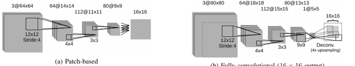
Fig. 1(a) illustrates the patch-based architecture from [29]. The network takes 64 × 64 patches (on color images of 1m2 spatial resolution) and predicts 16 × 16 centered patches of the same resolution. Three convolutional layers learn 64, 112 and 80 convolution kernels, of 12 × 12, 4 × 4 and 3 × 3 spatial dimensions, respectively. The first convolution is strided (one
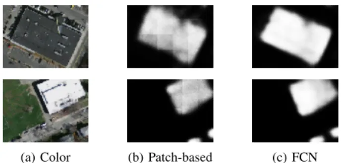
(a) Color (b) Patch-based (c) FCN
Fig. 2: The patch-based predictions exhibit artifacts on the patch borders while the FCN prevents them by construction.
convolution every four pixels), which implies a downsampling with factor 4.
After the three convolutional layers, a fully connected layer transforms the high-level features of the last convolutional layer into a classification map of 256 elements, matching the required 16 × 16 output patch.
Training is performed by selecting random patches from the training set, and grouping them into mini-batches as required by the stochastic gradient descent algorithm.
B. Limitations of the Patch-based Framework
We now point out some limitations of the patch-based approach discussed above, which motivate the design of an improved network architecture. Let us first analyze the role of the last fully connected layer that constructs the output patches. In the architecture of Fig. 1(a), the size of the feature maps in the last convolutional layer (before the last fully connected one) is 9 × 9. The resolution of these filters is 1/4 of the resolution of the input image, due to the 4-stride in the first convolution. The output of the fully connected layer is, however, a full-resolution 16 × 16 classification map. This means that the fully connected layer does not only compute the classification scores, but also learns how to upsample them. Outputting a full-resolution patch is then the result of upsampling and not of an intrinsic high-resolution processing. We also observe that the fully connected layer allows outputs at different locations to have different weights with respect to the previous layer. For example, the weights associated to an output pixel at the top-left corner of a patch can be different to those of a pixel at the bottom right. In other words, the network can learn priors on the position inside a patch. This makes sense in some specific contexts such as when labeling pictures of outdoor scenes: the system could learn a prior for the sky to be at the top of the image. In our context, however, the partition of an image into patches is arbitrary, hence the “in-patch location” prior is irrelevant since allowing different weights at different patch locations may yield undesirable properties. For example, feeding two image patches that are identical but rotated by 90 degrees could yield different classification maps.
When training the network of Fig. 1(a) we expect that, after processing many training cases, the fully connected layer will end up learning a location-invariant function. Figs. 2(a)-(b) illustrate a fragment of an output score map by using such
(a) Patch-based
(b) Fully convolutional (16 × 16 output)
Fig. 1: Convolutional neural network architectures (e.g., “64@14 × 14” means 64 feature maps of size 14 × 14).
an architecture. Notice the discontinuities at the border of the patches, which reveal that the network did not succeed in learning to classify pixels independently of their location inside the patch. While this issue is partly addressed in [29] by smoothing the outputs with a conditional random field, we argue that avoiding such artifacts by construction is desirable. In addition, generating similar results regardless of image tiling is an important property for large-scale satellite image processing, and an active research topic [31], [32]. Another concern with the fully connected layer is that the receptive field of every patch output is not centered in itself. For example, a prediction near the center of the output patch can “see” about 32 pixels in every direction around it. However, the prediction at the top-left corner of the output patch considers a larger portion of the image to the bottom and to the right than to the top and to the left. Considering that the division into patches is arbitrary, this behavior is hard to justify.
A deeper understanding of the role played by every layer of the network, as described in this section, motivates the design of a more suitable architecture from a theoretical point of view, with the additional goal of boosting the overall performance of the approach.
C. Fully Convolutional Network
We propose a fully convolutional neural network architec-ture (FCN) to produce dense predictions. We explicitly restrict the process to be location-independent, enforcing the outputs to be the result of a series of convolutions only (see Fig. 1b). A classification network may be “convolutionalized” [33] as follows. We first convert the fully connected layer that carries out the classification to a convolutional layer. The convolution kernel is chosen so that its dimensions coincide with the previous layer. Thus, its connections are equivalent to a fully connected layer. The difference is that if we enlarge the input image, the output size is also increased, but the number of parameters remains constant. This may be seen as convolving the whole original network around a larger image to evaluate the output at different locations.
To increase the resolution of the output map, we then add a so-called “deconvolutional” layer [33]. The goal of this layer is to upsample the feature maps from the previous layer, which is achieved by performing an interpolation from a set of nearby points. Such an interpolation is parametrized by a kernel that expresses the extent and amount of contribution from a pixel value to its neighboring positions, only based on their locations. For an effective interpolation, the kernels must be
Fig. 3: “Deconvolution” layer for upsampling.
large enough to overlap in the output. The interpolation is then performed by multiplying the values of the kernel by every input and adding the overlapping responses in the output. This process is illustrated by Fig. 3 for a 2x upsampling. Notice that the scaling step is performed based on a constant 4 × 4 kernel. In our framework, and as in previous work [33], the interpolation kernel is another set of learnable parameters of the network instead of being determined a priori, e.g., setting them to represent a bilinear interpolation. Note also that the upsampled feature map has a central part computed by adding the contribution of two neighboring kernels and an outer border obtained solely by the contribution of one kernel (the two leftmost and rightmost output columns in Fig. 3). The outer border can be seen as an extrapolation of the input while the inner part can be seen as an interpolation. The extrapolated border can be cropped from the output to avoid artifacts.
As compared to a patch-based approach, we can expect our fully convolutional network to exhibit the following advan-tages:
• Elimination of discontinuities due to patch borders;
• Improved accuracy due to a simplified learning process, with a smaller number of parameters;
• Lower execution time at inference, due to the fast GPU execution of convolution operations.
Our FCN network is constructed by convolutionalizing the existing patch-based network depicted by Fig. 1(a). We choose an existing framework to benefit from a mature architecture and to carry out a rigorous comparison. The architectural decisions (i.e., the choice of the number of layers and filter sizes) of the base network are described in [29].
Fig. 1(b) depicts the resulting FCN. First, we pretend that the output patch of the original network is only of size
1 × 1, thus just focusing on a single output centered in its receptive field. Second, we rewrite the fully connected layer as a convolutional layer with one feature map and the spatial dimensions of the previous layer (9 × 9). Third, we add a deconvolutional layer that upsamples its input by a factor of 4 (with a learnable kernel of size 8 × 8), in order to recover the input resolution. Notice that the tasks of classification and upsampling are now separated.
This new network can take input images of different sizes, with the output size varying accordingly. For example, during the training stage we wish to output patches of size 16 × 16 in order to emulate the learning process as was done in the patch-based network of Fig. 1(a). For this we require a patch input of size 80 × 80, as in the architecture of Fig. 1(b). Notice that the input is larger than the original 64 × 64 patches. This is not because we are taking more context to carry out the predictions, but instead because every output is now centered in its context. At inference time we can take inputs of arbitrary sizes and feed them to the network to construct the classification maps, and the number of network parameters does not vary.
In the deconvolutional layer illustrated in Fig. 1(b), the overlapping areas added to produce the output are depicted in gray while the excluded extrapolation is in white.
D. Experiments on Fully Convolutional Networks
We implemented the CNNs using the Caffe deep learning framework [34]. In a first experiment we apply our approach to the Massachusetts Buildings Dataset [29]. This dataset consists of color images over the area of Boston with 1 m2 spatial resolution, covering an area of 340 km2 for training,
9 km2for validation and 22.5 km2for testing. The images are
labeled into two classes: building and not building. A portion of an image and its corresponding reference are depicted in Figs. 4(a-b).
We train the patch-based and fully convolutional networks (Figs. 1(a) and 1(b) respectively) for 30,000 stochastic gra-dient descent iterations, until we observe barely no further improvement on the validation set. The patches are sampled uniformly from the whole training set, with mini-batches of 64 patches each and a learning rate of 0.0001. A momentum and an L2 parameter penalty are introduced to regularize the learning process and avoid overfitting. Momentum adds a fraction of the previous gradient to the current one in order to smooth the descent, while an L2 penalty on the learned parameters discourages neurons to specialize too much on particular training cases [30]. The weights of these regularizers are set to 0.9 and 0.0002 respectively. Further details on these so-called hyperparameters and rationale for selecting them are provided by Mnih [29].
To evaluate the accuracy of the classification we use two different measures: pixelwise accuracy (proportion of correctly classified pixels, obtained through binary classification of the output probabilities with threshold 0.5) and area under the receiver operating characteristics (ROC) curve [35]. The latter quantifies the relation between true and false positives at different thresholds, and is appropriate to evaluate the overall quality of the fuzzy maps.
Fig. 5(a) plots the evolution of the area under ROC curve and pixelwise accuracy in the test set, across iterations. The FCN consistently outperforms the patch-based network. Fig. 5(b) shows ROC curves for the final networks after convergence, the FCN exhibiting the best relation between true and false positive rates. Fig. 4(c-d) depicts some visual results. To further illustrate the benefits of neural networks over other learning approaches we train a support vector machine (SVM) with Gaussian kernel on 1,000 randomly selected pixels of each class. We train on the individual pixel spec-tra without any feature selection. The SVM parameters are selected by 5-fold cross-validation, as commonly performed in remote sensing image classification [10]. As shown by Fig. 4(e), the pixelwise SVM classification often confuses roads with buildings due to the fact that their colors are similar, while neural networks better infer and separate the classes by taking into account the geometry of the context. The accuracy of the SVM on the Boston test dataset is 0.6229 and its area under ROC curve is 0.5193, i.e., significantly lower than with CNNs, as shown in Fig. 5. If we wished to successfully use an SVM for this task, we should design and select spatial features (e.g., texture) and use them as the input to the classifier instead. The amplified fragment in Fig. 2 shows that the border discontinuity artifacts present in the patch-based scheme are absent in our fully convolutional setting. This behaves as expected considering that the issues described in Section III-B are addressed by construction in the new architecture. This confirms that imposing sensible restrictions to the connections of a neural network has a positive impact in the performance. In terms of efficiency the FCN also outperforms the patch-based CNN. At inference time, instead of carrying out the prediction in a small patch basis, the input of the FCN is simply increased to output larger predictions, better benefiting from the GPU parallelization of convolutions. The execution time required to classify the whole Boston 22.5 km2 test set
(performed on an Intel I7 CPU @ 2.7Ghz with a Quadro K3100M GPU) is 82.21 s with the patch-based CNN against 8.47 s with the FCN. The speedup is about 10x, a relevant im-provement considering the large-scale processing capabilities required by new sensors.
IV. END-TO-ENDFRAMEWORK
In remote sensing image analysis it is a common practice to train classifiers on the spectrum of a small number (a couple of hundreds) of isolated sample pixels [36]. Training relies on the trustworthiness of the reference data and on the fact that classes are reliably separable simply by observing the spectral signature of the sampled pixels. While such training approaches are popular, for example, in hyperspectral image classification, our goals differ as we wish to automatically learn contextual features that can help better identify the classes in satellite imagery. Our goal requires more training data per se, as we must show the classifier the many different contexts in which a pixel class can be embedded, and not just its spectral values. In addition, is it well-known that massive data might be required to train neural networks, contrary to a common feature selection and classification approach. This
(a) Color image (b) Reference data (c) Patch-based fuzzy map (d) FCN fuzzy map (e) SVM fuzzy map
Fig. 4: Experimental results on a fragment of the Boston dataset.
0.5 1 1.5 2 2.5 3 x 10⁴ 0.78 0.8 0.82 0.84 0.86 0.88 0.9 0.92 0.94 Iterations
Area under ROC curve Fully convolutional Patch−based 0.5 1 1.5 2 2.5 3 x 10⁴ 0.8 0.82 0.84 0.86 0.88 0.9 0.92 Iterations Pixel−wise accuracy Fully convolutional Patch−based
(a) Performance evolution
0 0.1 0.2 0.3 0.4 0.5 0.5 0.6 0.7 0.8 0.9 1
False Positive rate
True Positive rate
Patch−based Fully convolutional
(b) ROC curves
Fig. 5: Evaluation of patch-based and fully convolutional neural networks on the Boston test set.
led us to analyze and address the dependency of the algorithm on the availability and accuracy of the training data.
In the experiments described in Section III-D, the Mas-sachusetts Buildings dataset is used for training and testing. This dataset is a hand-corrected version of the OpenStreetMap (OSM) vectorial map available over the area covered by the images. Despite the existence of some inaccuracies in the reference data, the coverage of OSM in that region is satisfactory and the errors are minor.
In many other areas of Earth, however, the coverage of OSM is limited. In the samples of Fig. 8 we observe large areas with missing data and a general misregistration of the vectorial maps with respect to the actual structures. In addition, the misregistration is not uniform and neighboring buildings are often shifted in different directions. Note that in the samples of Fig. 8 the buildings have been delineated in OSM based on the official French cadaster records. However, even the cadaster records are not always accurate up to the meter resolution. Furthermore, satellite images undergo a series of corrections before being aligned to the maps. For example, the use of inexact elevation models for orthorectification might introduce misregistrations throughout the images. As a result, the OSM raw data is imperfect and thus not fully reliable.
The reference data obtained from OSM, as shown by Fig. 8, provides a rough idea of the location of the buildings, but rarely outlines them. In such a setting, convolutional neural networks would hardly learn that building boundaries are likely to fall on visible edges, since this is not what the refer-ence data depicts. Under these circumstances, we expect the predictions not to be very confident, especially on the border of the objects. As we will illustrate in Section IV-C, this yields a
“blobby” and overly fuzzy aspect to predictions obtained with the network of Section III-C on more challenging datasets.
Our first contribution in this section is a novel approach for tackling the issue of inaccurate labels for CNN training. For this we propose a two-step approach: 1) the network is first trained on raw OSM data, 2) it is then fine-tuned on a tiny piece of manually labeled image.
This method provides us with a means to deal with the inaccuracy of training data, by increasing the confidence and sharpness of the predictions. However, we still cannot expect it to provide highly precise boundaries with the fully convolutional architecture as described in Section III-C. This is because such network includes a downsampling step, re-quired to capture the long-range spatial dependencies that help recognize the classes. However, downsampling makes the whole system lose spatial precision, and the deconvo-lutional layer learns a way of naively upsampling the data from a restricted number of neighbors, without reincorporating higher-resolution information. What is lost in spatial precision through the network, is not recovered. This is a consequence of a well-known trade-off between the receptive field (how much context is taken to conduct predictions) and the output resolution (how fine is the prediction) if we wish to keep a reasonable number of trainable parameters [33]. Our second contribution is then a new architecture that incorporates infor-mation at multiple scales in order to alleviate this trade-off. Our architecture combines low-resolution long-range features with high-resolution local features that conduct predictions with a higher level of detail. This architecture, when combined with our two-step training approach, provides a framework that can be used end-to-end to classify satellite imagery.
A. Fine-tuning
Fine-tuning is a very common procedure in the neural network literature. The idea is to adapt an existing pretrained model to a different domain by executing a few training iter-ations on a new dataset. The notion of fine-tuning is based on the intuition that low-level information/features can be reused in different applications, without training from scratch. Even when the final classification objective is different, it is also a relevant approach for initializing the learnable parameters close to good local minima, instead of initializing with random weights. After proper fine-tuning, low-level features tend to be quite preserved from one dataset to another, while the higher layers’ parameters are updated to adapt the network to the new problem [37].
When fine-tuning, the training set for the new domain is usu-ally substantiusu-ally smaller than the one used to train the original network. This is because one assumes that some generalities of both domains are well conveyed in the pretrained network (e.g., edge detectors in different directions) and the fine-tuning phase is just needed to conduct the domain adaptation. When the training set used for fine-tuning is very small, additional considerations to avoid overfitting are commonly taken, such as early stopping (executing just a few iterations on the new training dataset), fixing the weights at the lower layers or reducing the learning rate.
We now incorporate the idea of neural network fine-tuning, in order to perform training on imperfect data. Our approach proceeds in two steps. In step one large amounts of training data are used to train a fully convolutional neural network. This raw training data is extracted directly from OSM, without any hand correction. The goal of this step is to capture the generalities of the dataset such as, e.g., the representative spectrum of object classes.
In step two, we fine-tune the network by using a small part of carefully labeled image. This phase is designed to compensate for the inaccuracy of labels obtained in step one, by fine-tuning the network on small yet consistent target outputs. Assuming that most of the generalities have been captured during the initial training step, the fine-tuning step should locally correct the network parameters to output more accurate classifications. The efforts of fine-tuning are thus limited to manually labeling a small dataset, while the large inaccurate dataset is automatically extracted from OSM.
B. Conducting Fine Predictions
The resolution at which the networks proposed in Section III operate yields probability maps that, once upsampled, are coarse in terms of spatial accuracy. A naive way to increase the resolution of the network would be to use higher-resolution filters, which requires to increase their dimensions if we want to preserve the receptive field. For example, instead of applying a 5 × 5 filter at a fourth of the image resolution, one could use a 20 × 20 filter at full resolution, hence covering the same spatial extent. However, such an increase in filter sizes is prohibitive, hampering the spatial and temporal efficiency of the algorithm and producing less accurate results due to the difficulty of optimizing so many parameters.
Nevertheless, we observed that we do not need full-resolution filters to conduct accurate predictions. One requires a higher resolution only in the center of the convolution filters (assuming that the pixel we wish to predict is in the center of the context of interest). A large spatial extent is indeed required to capture contextual information, but it is not necessary to conduct this analysis at full resolution. For example, the presence of two parallel bands of grass can help identify a road (and distinguish it from, for instance, a building with a gray rooftop), but a precise localization of the grass is not necessary. On the contrary, at the center of the convolution filter, a higher-resolution analysis is required to specifically locate the boundary of the aforementioned road.
Fig. 6 illustrates this observation. In Fig. 6(a) we observe the area around a pixel whose class we wish to predict, at full resolution. A filter taking such an amount of context with that resolution would be prohibitive in the number of parameters, as well as unnecessary. Fig. 6(b) depicts the same context at a quarter of the resolution. Notice that it is still possible to visually infer that there is a road. However, identifying the precise location of the boundaries of the road becomes difficult. Alternatively, Fig. 6(c) depicts a small patch but at full resolution. We can now better locate the precise boundary of the object, but with so little context it is difficult to identify that the object is indeed a road. Large filters at low resolution - see Fig. 6(b) or small filters at high resolution - see Fig. 6(c), which would both have a reasonable number of parameters, are bad alternatives: the first filter is too coarse and the second filter is using too little context.
We propose convolutional filters that combine multiple scales instead. In Fig. 6(d) the large-size low-resolution con-text of Fig. 6(b) is combined with the small high-resolution context of 6(d). This provides us with a means to simultane-ously infer the class by observing the surroundings at a coarse scale, and determine the precise boundary location by using a finer context. This way, the amount of parameters are kept small while the trade-off between recognition and localization is alleviated.
Les us denote by S a set of levels of detail expressed as a fraction of the original resolution. For example, S = {1, 1/2} is a set comprising two-scales: full resolution and half of the full resolution. We denote by xsa feature map x downsampled
to a certain level s ∈ S. For example, x1/2 is a feature map
downsampled to half of the original resolution. Inspired in Equation 1, we design a special type of neuron that adds the responses to a set of filters applied at different scales of the feature maps in the previous layer:
a = σ X
s∈S
wsxs+ b
!
. (5)
Notice that individual filters ws are learned for every scale
s. Such a filter is easily implemented by using a combination of elementary convolutional, downsampling and upsampling layers. Fig. 7 illustrates this process in the case of a two-scale (S = {1, 1/2}) module. In our implementation we average neighboring elements in a window for downsampling and perform bilinear interpolation for upsampling, but other
(a) Large context, high res-olution
(b) Large context, low res-olution
(c) Small context, high res-olution
(d) Combined scales
Fig. 6: Different types of context to predict a pixel’s class. A multi-scale context such as in (d) alleviates the trade-off between classification accuracy and number of learnable parameters.
Fig. 7: Two-scale convolutional module that simultaneously combines coarse large-range and fine short-range reasoning.
Fig. 8: Fragments of the Forez training set (red: building).
approaches are also applicable. The kernel sizes of the con-volutions at both scales are set to be equal (e.g., 3 × 3), yet the amount of context taken varies from one path to the other due to the different scales. The addition is an elementwise operation, followed by the nonlinear activation function.
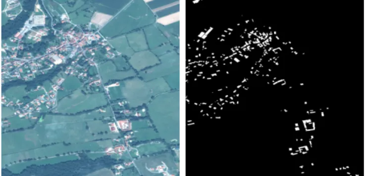
C. Experiments on the End-to-End Classification Framework We conduct our experiments on a Pl´eiades image over the area of Forez, France. An orthorectified color pansharpened version of the image is used, at a spatial resolution of 0.5 m2. Our training subset amounts to 22.5 km2. The criterion to construct the training set was to choose ten 3000 × 3000 tiles with at least some coverage of OpenStreetMap (OSM). The shape files were rasterized with GDAL1 to create the binary reference maps. Fig. 8 shows some fragments of the reference data. Inconsistent misregistrations and considerable omissions are observed all over.
1http://www.gdal.org
Fig. 9: Manually labeled tile for fine-tuning (3000×3000).
Fig. 10: Fragment of the fine-tuning tile. Red borders enclose building areas.
We manually labeled a 2.25 km2 tile for FCN fine-tuning, and a different 2.25 km2 tile for testing. The manual labeling takes about two hours for each of the tiles. The entire tuning tile is depicted by Fig. 9 and a close-up is shown in Fig. 10. The fully convolutional network (FCN) described in Section III-C, which was used for the Massachusetts dataset, is now trained with the Forez set, under a similar experimental setting. Note that this FCN was designed for images which have a 1 m2 resolution, while Pl´eiades imagery features a 0.5 m2
resolution. In order for the architectural decisions of FCN to be valid in our new dataset, one must preserve the receptive field size in terms of meters, not pixels. We thus downsample Pl´eiades images prior to entering the first layer of the FCN, and bilinearly upsample the output classification maps. Even though a new network directly tailored to the Pl´eiades reso-lution could be designed, we favor this proven architecture to conduct our experiments. The concepts described in this paper
Method Accuracy AUC IoU FCN 0.99126 0.99166 0.48 FCN + Fine-tuning 0.99459 0.99699 0.66 Two-scale FCN 0.99129 0.98154 0.47 Two-scale FCN + Fine-tuning 0.99573 0.99836 0.72 TABLE I: Performance evaluation on the Pl´eiades test set.
are however general and can be used to design other networks. After training on the raw OSM Forez dataset, we fine-tune the weights on the manually labeled tuning tile. The training hyper-parameters are kept similar in the fine-tuning step, but an early stopping criterion interrupts it after 200 iterations.
To assess the performance of fine-tuning we use as criteria pixelwise accuracy and area under the ROC curve (AUC), as described in Section III-D. Since there are many more non-building pixels than non-building pixels in this dataset, these accu-racy measures might seem overly high, a well-known issue of pixelwise accuracy in imbalanced datsets [38]. We add then the intersection over union criterion (IoU), an object-based overlap measure typically used for imbalanced datasets [38]. In our case it is defined as the number of pixels labeled as buildings both in the classified image and in the ground truth, divided by the total amount of pixels labeled as such in either of them. These criteria are evaluated on the manually labeled test set, which is used neither for training nor for fine-tuning. The first two rows of Table I show that fine-tuning enhances the quality of the predictions in terms of accuracy, AUC and IoU. To confirm the significance of the accuracy, a McNemar’s test [39] proved that the improvement is not a result of mere luck with a probability greater than 0.99999. Besides, the IoU is improved by over a third with the fine-tuned network.
Fig. 11(a-d) shows the impact of fine-tuning on several amplified fragments of the test set. A greater confidence in the fine-tuned network predictions is observed. The objects exhibit better alignment to the objects of the image, albeit the boundaries could better line up to the underlying edges.
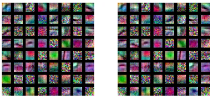
Fig. 12 illustrate the first-layer convolutional filters learned by the initial and fine-tuned networks. We observe a combina-tion of low- and high-frequency filters, a behavior typically observed in CNNs. We also observe edge and color blob detectors. These filter remain unchanged after fine-tuning, even though no constraints are introduced to enforce this. Fine-tuning corrects the weights in the high-level layers, which suggests that the initial low-level features were useful indeed, but the inaccuracy in the labels was introducing fuzziness in the upper layers of the network.
We now evaluate the performance of a two-scale network. The FCN architecture described in Section III-C is replaced by three two-scale stacked modules, with scales S = {1, 1/4}. We select S = 1/4 as it corresponds to the degree of downsampling of the original FCN network, and S = 1 is added to refine the predictions. The three modules learn 3 × 3 filters in both scales. The first two modules generate 64 feature maps and the last module generates a single map with the building/non-building prediction.
The two-scale network is trained and fine-tuned in a similar setting as the FCN network. The results summarized in the last two rows of Table I show that fine-tuning significantly
Fig. 12: First layer filters before and after fine-tuning.
enhances the classification performance, and that the fine-tuned two-scale network outperforms the single scale network. Notably, IoU goes from 0.48 to 0.72, implying that objects overlap with the ground truth 50% better by adding a scale and performing fine-tuning. Note that if a scale is added but no fine-tuning is done, there is actually a slight decrease in performance. A possible explanation for this is that including a finer scale adds even more confusion to the training algorithm if only noisy misregistered labels are provided.
Figs. 11(e-f) illustrate the results on visual fragments of the test set. The two-scale network yields classification maps that better correspond to the actual image objects, and exhibit sharper angles and straighter lines. The entire classified test tile for the fine-tuned two-scale network is depicted by Fig. 13c. The time required to generate this result corresponds to three hours for training on the OSM dataset, two hours to manually label an image tile and about a minute for fine-tuning. The prediction of the 3000 × 3000 test tile using the hardware described in Section III-D takes 3.2 seconds, and it grows linearly in the size of the image. As in Section III-D, we ran an SVM on the individual pixel values (see the classification map in Fig. 13b). Accuracy is 0.9487 and IoU 0.19, yielding poorer results than the presented CNN-based approaches.
As validated by the experiments, the issue of not having large amounts of high-quality reference data can be alleviated by providing the network with a small amount of accurate data in a fine-tuning step. Our multi-scale neurons combine reasoning at different resolutions to effectively produce fine predictions, while keeping a reasonable number of parameters. Such a framework can be used end-to-end to perform the classification task directly from input imagery. More scales can be easily be added and, besides the fact of being fully convolutional, there are little constraints on the architecture itself, admitting a different number of classes, input bands or number of feature maps.
V. CONCLUDINGREMARKS
Convolutional neural networks have become a popular clas-sifier in the context of image analysis due to their potential to automatically learn relevant contextual features. Initially devised for the categorization of natural images, these net-works must be revisited and adapted to tackle the problem of pixelwise labeling in remote sensing imagery.
We proposed a fully convolutional network architecture by analyzing a state-of-the-art model and solving its concerns by construction. Despite their outstanding learning capability, the
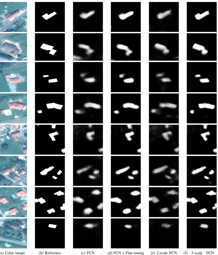
(a) Color image (b) Reference (c) FCN (d) FCN + Fine-tuning (e) 2-scale FCN (f) 2-scale FCN + Fine-tuning
Fig. 11: Classified fragments of the Pl´eiades test image. Fine-tuning increases the confidence of the predictions, and the two-scale network produces fine-grained classification maps.
(a) Color pansharpened input (b) SVM on individual pixels (c) FCN (two scales + fine-tuning) Fig. 13: Binary classification maps on the Forez test image.
lack of accurate training data might limit the applicability of CNN models in realistic remote sensing contexts. We therefore proposed a two-step training approach combining the use of large amounts of raw OpenStreetMap data and a small sample of manually labeled reference. The last ingredient we needed to provide a usable end-to-end framework for remote sensing image classification was to produce fine-grained classification maps, since typical CNNs tend to hamper the fineness of the output as a side effect of taking large amounts of context. We proposed a type of neuron module that simultaneously reasons at different scales.
Experiments showed that our fully convolutional network outperforms the previous model in multiple aspects: the accu-racy of the results is improved, the visual artifacts are removed and the inference time is reduced by a factor of ten. The use of our architecture constitutes then a win-win situation in which no aspect is compromised for the others. This was achieved by analyzing the role played by every layer in the network in order to propose a more appropriate architecture, showing that a deep understanding of how CNNs work is important for their success. Further experimentation showed that the two-step training approach effectively combines imperfect training data with manually labeled data to capture the dataset’s generalities and its precise details. Moreover, the multi-scale modules increase the level of detail of the classification without making the number of parameters explode, attenuating the trade-off between detection and localization.
Our overall framework shows then that convolutional neural networks can be used end-to-end to process large amounts of satellite images and provide accurate pixelwise classifications. As future work we plan to extend our experiments to multiple object classes and study the possibility of directly inputting non-pansharpened imagery, in order to avoid this preprocessing step. We also plan to study the introduction of shape priors in the learning process and the vectorization of the classification maps.
ACKNOWLEDGMENT
All Pl´eiades images are c CNES (2012 and 2013), distri-bution Airbus DS / SpotImage. The authors thank CNES for initializing and funding the study, and providing Pl´eiades data.
REFERENCES
[1] Yann LeCun, L´eon Bottou, Yoshua Bengio, and Patrick Haffner, “Gradient-based learning applied to document recognition,” Proceedings of the IEEE, vol. 86, no. 11, pp. 2278–2324, 1998.
[2] Dan Ciresan, Ueli Meier, and J¨urgen Schmidhuber, “Multi-column deep neural networks for image classification,” in IEEE CVPR, 2012, pp. 3642–3649.
[3] Alex Krizhevsky, Ilya Sutskever, and Geoffrey E Hinton, “Imagenet classification with deep convolutional neural networks,” in NIPS, 2012. [4] Annamalai Senthil Kumar and Kantilal Majumder, “Information fusion in tree classifiers,” International Journal of Remote Sensing, vol. 22, no. 5, pp. 861–869, 2001.
[5] Jean Mas and Juan Flores, “The application of artificial neural networks to the analysis of remotely sensed data,” International Journal of Remote Sensing, vol. 29, no. 3, pp. 617–663, 2008.
[6] Thomas Villmann, Erzsbet Mernyi, and Barbara Hammer, “Neural maps in remote sensing image analysis,” Neural Networks, vol. 16, no. 34, pp. 389 – 403, 2003, Neural Network Analysis of Complex Scientific Data: Astronomy and Geosciences.
[7] Gustavo Camps-Valls and Lorenzo Bruzzone, “Kernel-based methods for hyperspectral image classification,” IEEE Tran. Geosci. Remote Sens., vol. 43, no. 6, pp. 1351–1362, 2005.
[8] Mathieu Fauvel, Yuliya Tarabalka, Jon Atli Benediktsson, Jocelyn Chanussot, and James C Tilton, “Advances in spectral-spatial classi-fication of hyperspectral images,” Proceedings of the IEEE, vol. 101, no. 3, pp. 652–675, 2013.
[9] Wenzhi Liao, Mauro Dalla Mura, Jocelyn Chanussot, Rik Bellens, and Wilfried Philips, “Morphological attribute profiles with partial reconstruction,” IEEE Tran. Geosci. Remote Sens., vol. 54, no. 3, pp. 1738–1756, 2016.
[10] Yuliya Tarabalka and Aakanksha Rana, “Graph-cut-based model for spectral-spatial classification of hyperspectral images,” in IEEE IGARSS. IEEE, 2014, pp. 3418–3421.
[11] Mehmet Nadir Kurnaz, Zmray Dokur, and Tamer lmez, “Segmentation of remote-sensing images by incremental neural network,” Pattern Recognition Letters, vol. 26, no. 8, pp. 1096 – 1104, 2005.
[12] Christopher David Lloyd, Suha Berberoglu, Paul Curran, and Peter Atkinson, “A comparison of texture measures for the per-field classi-fication of mediterranean land cover,” International Journal of Remote Sensing, vol. 25, no. 19, pp. 3943–3965, 2004.
[13] Dengsheng Lu and Qihao Weng, “A survey of image classification methods and techniques for improving classification performance,” In-ternational journal of Remote sensing, vol. 28, no. 5, pp. 823–870, 2007. [14] ME Midhun, Sarath R Nair, VT Prabhakar, and S Sachin Kumar, “Deep model for classification of hyperspectral image using restricted boltz-mann machine,” in Proceedings of the 2014 International Conference on Interdisciplinary Advances in Applied Computing. ACM, 2014, p. 35. [15] Tong Li, Junping Zhang, and Ye Zhang, “Classification of hyperspectral
image based on deep belief networks,” in IEEE ICIP, 2014.
[16] Viktor Slavkovikj, Steven Verstockt, Wesley De Neve, Sofie Van Hoecke, and Rik Van de Walle, “Hyperspectral image classification with convo-lutional neural networks,” in Proceedings of the 23rd ACM international conference on Multimedia. ACM, 2015, pp. 1159–1162.
[17] Yushi Chen, Xing Zhao, and Xiuping Jia, “Spectral-spatial classification of hyperspectral data based on deep belief network,” IEEE J. Sel. Topics Appl. Earth Observ. in Remote Sens., vol. 8, no. 6, June 2015. [18] Yushi Chen, Zhouhan Lin, Xing Zhao, Gang Wang, and Yanfeng Gu,
“Deep learning-based classification of hyperspectral data,” IEEE J. Sel. Topics Appl. Earth Observ. in Remote Sens., vol. 7, no. 6, pp. 2094– 2107, 2014.
[19] Jun Yue, Wenzhi Zhao, Shanjun Mao, and Hui Liu, “Spectral–spatial classification of hyperspectral images using deep convolutional neural networks,” Remote Sensing Letters, vol. 6, no. 6, pp. 468–477, 2015. [20] Konstantinos Makantasis, Konstantinos Karantzalos, Anastasios
Doulamis, and Nikolaos Doulamis, “Deep supervised learning for hyperspectral data classification through convolutional neural networks,” in IEEE IGARSS. IEEE, 2015, pp. 4959–4962.
[21] Wenzhi Zhao and Shihong Du, “Spectral–spatial feature extraction for hyperspectral image classification: A dimension reduction and deep learning approach,” IEEE Tran. Geosci. Remote Sens., vol. 54, no. 8, pp. 4544–4554, 2016.
[22] Wenzhi Zhao, Zhou Guo, Jun Yue, Xiuyuan Zhang, and Liqun Luo, “On combining multiscale deep learning features for the classification of hyperspectral remote sensing imagery,” International Journal of Remote Sensing, vol. 36, no. 13, pp. 3368–3379, 2015.
[23] Wenzhi Zhao and Shihong Du, “Learning multiscale and deep repre-sentations for classifying remotely sensed imagery,” ISPRS Journal of Photogrammetry and Remote Sensing, vol. 113, pp. 155–165, 2016. [24] Essa Basaeed, Harish Bhaskar, Paul Hill, Mohammed Al-Mualla, and
David Bull, “A supervised hierarchical segmentation of remote-sensing images using a committee of multi-scale convolutional neural networks,” International Journal of Remote Sensing, vol. 37, no. 7, 2016. [25] Jun Wang, Jingwei Song, Mingquan Chen, and Zhi Yang, “Road network
extraction: a neural-dynamic framework based on deep learning and a finite state machine,” International Journal of Remote Sensing, vol. 36, no. 12, pp. 3144–3169, 2015.
[26] Xueyun Chen, Shiming Xiang, Cheng-Lin Liu, and Chun-Hong Pan, “Vehicle detection in satellite images by hybrid deep convolutional neural networks,” IEEE Geoscience and remote sensing letters, vol. 11, no. 10, pp. 1797–1801, 2014.
[27] Igor ˇSevo and Aleksej Avramovi´c, “Convolutional neural network based automatic object detection on aerial images,” IEEE Geoscience and Remote Sensing Letters, vol. 13, no. 5, pp. 740–744, 2016.
[28] FPS Luus, BP Salmon, F Van Den Bergh, and BTJ Maharaj, “Multiview deep learning for land-use classification,” IEEE Geoscience and Remote Sensing Letters, vol. 12, no. 12, pp. 2448–2452, 2015.
[29] Volodymyr Mnih, Machine learning for aerial image labeling, Ph.D. thesis, University of Toronto, 2013.
[30] Christopher M Bishop, Neural networks for pattern recognition, Oxford university press, 1995.
[31] Julien Michel, David Youssefi, and Manuel Grizonnet, “Stable mean-shift algorithm and its application to the segmentation of arbitrarily large remote sensing images,” IEEE Tran. Geosci. Remote Sens., vol. 53, no. 2, pp. 952–964, 2015.
[32] Pierre Lassalle, Jordi Inglada, Julien Michel, Manuel Grizonnet, and Julien Malik, “A scalable tile-based framework for region-merging segmentation,” IEEE Tran. Geosci. Remote Sens., vol. 53, no. 10, pp. 5473–5485, 2015.
[33] Jonathan Long, Evan Shelhamer, and Trevor Darrell, “Fully convolu-tional networks for semantic segmentation,” in CVPR, 2015.
[34] Yangqing Jia, Evan Shelhamer, Jeff Donahue, Sergey Karayev, Jonathan Long, Ross Girshick, Sergio Guadarrama, and Trevor Darrell, “Caffe: Convolutional architecture for fast feature embedding,” arXiv preprint arXiv:1408.5093, 2014.
[35] C`esar Ferri, Jos´e Hern´andez-Orallo, and Peter A Flach, “A coherent interpretation of AUC as a measure of aggregated classification perfor-mance,” in ICML, 2011.
[36] Yuliya Tarabalka, Mathieu Fauvel, Jocelyn Chanussot, and J´on Atli Benediktsson, “Svm-and mrf-based method for accurate classification of hyperspectral images,” Geoscience and Remote Sensing Letters, IEEE, vol. 7, no. 4, pp. 736–740, 2010.
[37] Jason Yosinski, Jeff Clune, Yoshua Bengio, and Hod Lipson, “How transferable are features in deep neural networks?,” in NIPS, 2014. [38] Gabriela Csurka, Diane Larlus, Florent Perronnin, and France Meylan,
“What is a good evaluation measure for semantic segmentation?.,” in BMVC, 2013, vol. 27, p. 2013.
[39] Quinn McNemar, “Note on the sampling error of the difference between correlated proportions or percentages,” Psychometrika, vol. 12, no. 2, pp. 153–157, 1947.
Emmanuel Maggiori received the Engineering de-gree in computer science from Central Buenos Aires Province National University (UNCPBA), Tandil, Argentina, in 2014. The same year he joined AYIN and STARS teams at Inria Sophia Antipolis-M´editerran´ee as a research intern in the field of remote sensing image processing. Since 2015, he has been working on his Ph.D. within TITANE team, studying machine learning techniques for large-scale processing of satellite imagery.
Yuliya Tarabalka (S’08–M’10) received the B.S. degree in computer science from Ternopil Ivan Pul’uj State Technical University, Ukraine, in 2005 and the M.Sc. degree in signal and image processing from the Grenoble Institute of Technology (INPG), France, in 2007. She received a joint Ph.D. degree in signal and image processing from INPG and in electrical engineering from the University of Iceland, in 2010.
From July 2007 to January 2008, she was a researcher with the Norwegian Defence Research Establishment, Norway. From September 2010 to December 2011, she was a postdoctoral research fellow with the Computational and Information Sciences and Technology Office, NASA Goddard Space Flight Center, Greenbelt, MD. From January to August 2012 she was a postdoctoral research fellow with the French Space Agency (CNES) and Inria Sophia Antipolis-M´editerran´ee, France. She is currently a researcher with the TITANE team of Inria Sophia Antipolis-M´editerran´ee. Her research interests are in the areas of image processing, pattern recognition and development of efficient algorithms. She is Member of the IEEE Society.
Guillaume Charpiat is a researcher at Inria Saclay (France) in the TAO team. He studied Mathemat-ics and PhysMathemat-ics at the ´Ecole Normale Sup´erieure (ENS Paris), and then Computer Vision and Machine Learning (at ENS Cachan), as well as Theoretical Physics. His PhD thesis, in Computer Science, ob-tained in 2006, was on the topic of distance-based shape statistics for image segmentation with priors. He then spent one year at the Max-Planck Institute for Biological Cybernetics (T¨ubingen, Germany), on the topics of medical imaging (MR-based PET prediction) and automatic image colorization. As a researcher at Inria Sophia-Antipolis (France), he worked mainly on image segmentation and optimization techniques. Now at Inria Saclay he focuses on Machine Learning, in particular on building a theoretical background for neural networks.
Pierre Alliez Pierre Alliez is Senior Researcher and team leader at Inria Sophia-Antipolis - Mediterranee. He has authored scientific publications and several book chapters on mesh compression, surface recon-struction, mesh generation, surface remeshing and mesh parameterization. He is an associate editor of the Computational Geometry Algorithms Library (http://www.cgal.org) and an associate editor of the ACM Transactions on Graphics. He was awarded in 2005 the EUROGRAPHICS young researcher award for his contributions to computer graphics and geometry processing. He was co-chair of the Symposium on Geometry Processing in 2008, of Pacific Graphics in 2010 and Geometric Modeling and Processing 2014. He was awarded in 2011 a Starting Grant from the European Research Council on Robust Geometry Processing.