HAL Id: halshs-00175929
https://halshs.archives-ouvertes.fr/halshs-00175929
Submitted on 1 Oct 2007
HAL is a multi-disciplinary open access archive for the deposit and dissemination of sci-entific research documents, whether they are pub-lished or not. The documents may come from teaching and research institutions in France or abroad, or from public or private research centers.
L’archive ouverte pluridisciplinaire HAL, est destinée au dépôt et à la diffusion de documents scientifiques de niveau recherche, publiés ou non, émanant des établissements d’enseignement et de recherche français ou étrangers, des laboratoires publics ou privés.
Asymptotic and bootstrap inference for inequality and
poverty measures
Russell Davidson, Emmanuel Flachaire
To cite this version:
Russell Davidson, Emmanuel Flachaire. Asymptotic and bootstrap inference for inequality and poverty measures. Econometrics, MDPI, 2007, 141 (1), pp.141-166. �10.1016/j.jeconom.2007.01.009�. �halshs-00175929�
Asymptotic and Bootstrap Inference for
Inequality and Poverty Measures
by
Russell Davidson
Department of Economics McGill University Montreal, Quebec, Canada
H3A 2T7
GREQAM
Centre de la Vieille Charit´e 2 rue de la Charit´e 13002 Marseille, France email: [email protected]
and
Emmanuel Flachaire
Eurequa, Universit´e Paris I Panth´eon-Sorbonne
Maison des Sciences ´Economiques
106-112 bd de l’Hopital 75647 Paris Cedex 13
Abstract
A random sample drawn from a population would appear to offer an ideal opportunity to use the bootstrap in order to perform accurate inference, since the observations of the sample are IID. In this paper, Monte Carlo results suggest that bootstrapping a commonly used index of inequality leads to inference that is not accurate even in very large samples, although inference with poverty indices is satisfactory. We find that the major cause is the extreme sensitivity of many inequality indices to the exact nature of the upper tail of the income distribution. This leads us to study two non-standard bootstraps, the m out of n bootstrap, which is valid in some situations where the standard bootstrap fails, and a bootstrap in which the upper tail is modelled paramet-rically. Monte Carlo results suggest that accurate inference can be achieved with this last method in moderately large samples.
JEL codes: C00, C15, I32
Key words: Income distribution, poverty, bootstrap inference
This paper is a part of the research program of the TMR network “Living Standards, Inequality and Taxation” [Contract No. ERBFMRXCT 980248] of the European Communities, whose financial support is gratefully acknowledged. This research was also supported, in part, by a grant from the Social Sciences and Humanities Research Council of Canada. We thank seminar participants at the Montreal Statistics seminar, the ESRC Econometric Study Group, ITAM (Mexico), and Syracuse University for helpful comments. Remaining errors are ours.
1. Introduction
Statistical inference for inequality and poverty measures has been of considerable in-terest in recent years. It used to be thought that, in income analyses, we often deal with very large samples, and so precision is not a serious issue. But this has been
contradicted by large standard errors in many empirical studies; see Maasoumi(1997).
Two types of inference have been developed in the literature, based on asymptotic and bootstrap methods. Asymptotic inference is now well understood for the vast majority
of measures; see Davidson and Duclos (1997) and (2000). A few studies on bootstrap
inference for inequality measures have been conducted, and the authors of these studies recommend the use of the bootstrap rather than asymptotic methods in practice (Mills
and Zandvakili (1997) and Biewen(2002)).
In this paper, we study finite-sample performance of asymptotic and bootstrap infer-ence for inequality and poverty measures. Our simulation results suggest that neither asymptotic nor standard bootstrap inference for inequality measures performs well, even in very large samples. We investigate the reasons for this poor performance, and find that inference, both asymptotic and bootstrap, is very sensitive to the exact nature of the upper tail of the income distribution. Real-world income data often give good fits with heavy-tailed parametric distributions, for instance the Generalized Beta, Singh-Maddala, Dagum, and Pareto distributions. A problem encountered with heavy-tailed distributions like these is that extreme observations are frequent in data sets, and it
is well known that extreme observations can cause difficulties for the bootstrap.1 We
propose the use of two non-standard bootstrap methods, a version of the m out of n bootstrap, and one in which tail behaviour is modelled parametrically, to improve finite-sample performance. Simulation results suggest that the quality of inference is indeed improved, especially when the second method is used.
The paper is organized as follows. Section 2 reviews method-of-moments estimation
of indices. Section 3 presents some Monte Carlo results on asymptotic and bootstrap
inference on the Theil inequality measure. Section 4 investigates the reasons for the
poor performance of the bootstrap. Section 5 provides Monte Carlo evidence on the
performance of the two newly proposed methods. Section 6 presents some results on
asymptotic and bootstrap inference based on the FGT poverty measure. Section 7
concludes.
2. Method-of-Moments Estimation of Indices
A great many measures, or indices, of inequality or poverty can be defined for a popu-lation. Most depend only on the distribution of income within the population studied. Thus, if we denote by F the cumulative distribution function (CDF) of income in the population, a typical index can be written as I(F ), where the functional I maps from the space of CDFs into (usually) the positive real line. With two populations, A and B, 1 The simulation results of Biewen(2002)suggest that the bootstrap performs well in finite samples. However, this author used a lognormal distribution in his simulations; since this distribution is not heavy-tailed, better results can be expected with this design.
say, we have two CDFs, that we denote as FA and FB, and we say that there is more
inequality, or poverty, depending on the nature of the index used, in A than in B, if
I(FA) > I(FB). The ranking of the populations depends, of course, on the choice of
index.
It is well known that whole classes of indices will yield a unanimous ranking of A and
B if a condition of stochastic dominance is satisfied by FA and FB. For instance, if
FA(y) ≥ FB(y) for all incomes y, with strict inequality for at least one y, then population
B is said to dominate A stochastically at first order. In that event, all welfare indices W of the form
W (F ) = Z
U (y) dF (y), (1)
where U is an increasing function of its argument, will unanimously rank B as better off than A. Similar results hold for higher-order stochastic dominance, and for poverty and inequality indices - for these, a higher value of the index in A corresponds to A being worse off than B.
Let Y denote a random variable with CDF F . A realization of Y is to be thought of as the income of a randomly chosen member of the population. Then many indices, like (1), are expressed as moments of a function of Y, or as a smooth function of a vector of such moments. All of the members of the class of Generalized Entropy indices are instances of this, as can be seen from their explicit form:
GEα(F ) = 1 α(α − 1) hEF(Yα) EF(Y )α − 1i,
where by EF(.) we denote an expectation computed with the CDF F . In this paper,
we treat the index GE1 in some detail. This index is also known as Theil’s index, and
it can be written as T (F ) = Z y µF log ³ y µF ´ dF (y) (2)
where the mean of the distribution µF ≡ EF(Y ) =R y dF (y). It is clear from (2) that
the index T is scale invariant. It is convenient to express Theil’s index as a function of
µF and another moment
νF ≡ EF(Y log Y ) =
Z
y log y dF (y). From (2) it is easy to see that
T (F ) = (νF/µF) − log µF.
If Yi, i = 1, . . . , n, is an IID sample from the distribution F , then the empirical
distri-bution function of this sample is ˆ F (y) = 1 n n X i=1 I(Yi≤ y), (3)
where the indicator function I(.) of a Boolean argument equals 1 if the argument is true, and 0 if it is false. It is clear that, for any smooth function f , the expectation of
f (Y ), EF[f (Y )], if it exists, can be consistently estimated by
EFˆ[f (Y )] = Z f (y) d ˆF (y) = 1 n n X i=1 f (Yi).
This estimator is asymptotically normal, with asymptotic variance
Var ¡n1/2{E
ˆ
F[f (Y )] − EF[f (Y )]}¢ = EF[f
2(Y )] − {E
F[f (Y )]}2,
which can be consistently estimated by
EFˆ[f2(Y )] − {EFˆ[f (Y )]}2.
The Theil index (2) can be estimated by
T ( ˆF ) ≡ (νFˆ/µFˆ) − log µFˆ. (4)
This estimate is also consistent and asymptotically normal, with asymptotic variance
that can be calculated by the delta method. Specifically, if ˆΣ is the estimate of the
covariance matrix of µFˆ and νFˆ, the variance estimate for T ( ˆF ) is
· −νFˆ + µFˆ µ2 ˆ F 1 µFˆ ¸ ˆ Σ −νFˆ + µFˆ µ2Fˆ 1 µFˆ (5)
3. Asymptotic and Bootstrap Inference
Armed with the estimate (4) and the estimate (5) of its variance, it is possible to test hypotheses about T (F ) and to construct confidence intervals for it. The obvious way to proceed is to base inference on asymptotic t-type statistics computed using (4) and (5).
Consider a test of the hypothesis that T (F ) = T0, for some given value T0. The
asymptotic t-type statistic for this hypothesis, based on ˆT ≡ T ( ˆF ), is
W = ( ˆT − T0)/[ ˆV ( ˆT )]1/2, (6)
where by ˆV ( ˆT ) we denote the variance estimate (5).
We make use of simulated data sets drawn from the Singh-Maddala distribution, which can quite successfully mimic observed income distributions in various countries, as
shown by Brachman, Stich, and Trede (1996). The CDF of the Singh-Maddala
dis-tribution can be written as
F (y) = 1 − 1
We use the parameter values a = 100, b = 2.8, c = 1.7, a choice that closely mimics the net income distribution of German households, apart from a scale factor. It can be shown that the expectation of the distribution with CDF (7) is
µF = ca−1/b
Γ(b−1+ 1)Γ(c − b−1)
Γ(c + 1) and that the expectation of Y log Y is
µF b−1[ψ(b−1+ 1) − ψ(c − b−1) − log a]
where ψ(z) ≡ Γ′(z)/Γ(z) is the digamma function - see Abramowitz and Stegun(1965),
page 258. For our choice of parameter values, we have µF = 0.168752, νF = −0.276620,
and, from (2), that T (F ) = 0.140115.
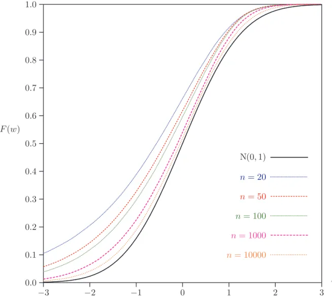
InFigure 1, we show the finite sample CDFs of the statistic W calculated from samples
of N = 10,000 independent drawings from (7), with T0 given by the value T (F ) and
n = 20, 50, 100, 1,000 and 10,000. For comparison purposes, the CDF of the nominal N(0, 1) distribution is also shown. It is clear that the nominal distribution of the t-type statistic is not at all close to the finite sample distribution in small and moderate samples, and that the difference is still visible in huge samples.
The dismal performance of the asymptotic distribution discussed above is quite enough to motivate a search for better procedures, and the bootstrap suggests itself as a nat-ural candidate. The simplest procedure that comes to mind is to resample the original data, and then, for each resample, to compute whatever test statistic was chosen for the purposes of inference. Since the test statistic we have looked at so far is asymptot-ically pivotal, bootstrap inference should be superior to asymptotic inference because
of Beran’s (1988) result on prepivoting. Suppose, for concreteness, that we wish to
bootstrap the t-type statistic W of (6). Then, after computing W from the observed sample, one draws B bootstrap samples, each of the same size n as the observed
sam-ple, by making n draws with replacement from the n observed incomes Yi, i = 1, . . . , n,
where each Yi has probability 1/n of being selected on each draw. Then, for bootstrap
sample j, j = 1, . . . , B, a bootstrap statistic W⋆
j is computed in exactly the same way
as was W from the original data, except that T0in the numerator (6) is replaced by the
index ˆT estimated from the original data. This replacement is necessary in order that
the hypothesis that is tested by the bootstrap statistics should actually be true for the population from which the bootstrap samples are drawn, that is, the original sample. Details of the theoretical reasons for this replacement can be found in many standard
references, such as Hall (1992). This method is known as the percentile-t or bootstrap-t
method.
Bootstrap inference is most conveniently undertaken by computing a bootstrap P value;
see for instance Davidson and MacKinnon (1999). The bootstrap P value is just the
proportion of the bootstrap samples for which the bootstrap statistic is more extreme than the statistic computed from the original data. Thus, for a one-tailed test that
rejects when the statistic is in the left-hand tail, the bootstrap P value, P⋆, is
P⋆ = 1 B B X j=1 I(Wj⋆ < W ), (8)
where I(.) is once more an indicator function. It is more revealing for our purposes to consider one-tailed tests with rejection when the statistic is too negative than the usual two-tailed tests, the reason being that the leftward shift of the distribution seen inFigure 1 means that the worst behaviour of the statistic occurs in the left-hand tail.
Mills and Zandvakili (1997)introduced the bootstrap for measures of inequality using
the percentile method, which bootstraps the statistic ˆT . However, the percentile method
does not benefit from Beran’s refinement, because the statistic bootstrapped is not
asymptotically pivotal. Note that a percentile bootstrap P value is computed with W⋆
j
and W respectively replaced by ˆT⋆
j − ˆT and ˆT − T0 in (8). A test based on such a
P value is referred to as a percentile test in our experiments.
Using Edgeworth expansions, van Garderen and Schluter (2001) show that the actual
distribution of the statistic W is biased to the left, as we have seen in Figure 1. They
suggest shifting the distribution by adding the term n−1/2c to the statistic, where c
is a constant estimated using Gaussian kernel density methods and with a bandwidth obtained automatically by cross-validation. Rather than using kernel density methods
to estimate this bias, we use bootstrap methods, approximating n−1/2c by the mean of
the B bootstrap statistics Wj⋆, j = 1 . . . B. Then, we compute the bootstrap bias-shifted
statistic, W′′ = W − B−1 B X j=1 Wj⋆ (9)
of which the distribution should be closer to the standard normal distribution used to compute an asymptotic P value.
Given the leftward bias of all the statistics considered so far, we can expect that, in their asymptotic versions, one-tailed tests that reject to the left will systematically overreject. InFigure 2, this can be seen to be true for bootstrap and asymptotic tests for different sample sizes n = 20, 50, 100, 500, 1,000, 2,000, 3,000, 4,000, and 5,000. This figure shows errors in rejection probability, or ERPs, of asymptotic and bootstrap tests at nominal level α = 0.05, that is, the difference between the actual and nominal probabilities of rejection. A reliable statistic, that is, one that yields tests with no size distortion, would give a plot coincident with the horizontal axis. In our simulations, the number of Monte Carlo replications is N = 10,000 and the number of bootstrap replications is B = 199. This figure has the following interesting features:
(1) The ERP of the asymptotic test is very large in small samples, and is still significant in very large samples: for n = 5,000, the asymptotic test over-rejects the null hypothesis with an ERP of 0.0307, and thus an actual rejection probability of 8.07% when the nominal level is 5%.
(2) The ERP of the percentile bootstrap method turns out to be close to the ERP of the asymptotic test. As we could have expected, and as the simulation results of
Mills and Zandvakili (1997), and van Garderen and Schluter (2001) indicate, our
results show that asymptotic and percentile bootstrap tests perform quite similarly in finite samples, and their poor performance is still visible in very large samples.
(3) The ERP of the bootstrap bias shifted test W′′ defined in (9) is much less than for
the asymptotic test, but is higher than for the percentile-t bootstrap test.
(4) Despite an ERP of the percentile-t bootstrap method that is clearly visible even in large samples, it can be seen that the promise of the bootstrap approach is borne out to some extent: the ERP of the percentile-t bootstrap is much less than that of any of the other methods.
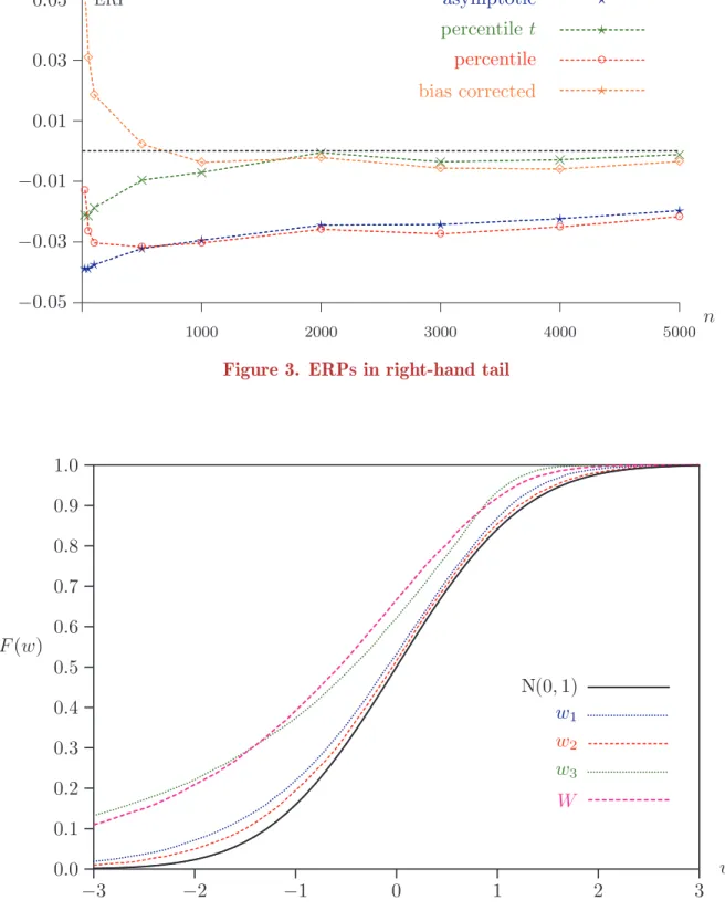
One-tailed tests that reject to the right can be expected to have quite different
proper-ties. This can be see in Figure 3, in which we see that the ERPs are considerably less
than for tests rejecting to the left. Note that these ERPs are computed as the excess rejection in the right-hand tail. For sample sizes less than around 500, the bias-shifted test overrejects significantly.
4. Reasons for the poor performance of the bootstrap
In this section, we investigate the reasons for the poor performance of the bootstrap, and discuss three potential causes. First, almost all indices are nonlinear functions of sample moments, thereby inducing biases and non-normality in estimates of these indices. Second, estimates of the covariances of the sample moments used to construct indices are often very noisy. Third, the indices are often extremely sensitive to the exact nature of the tails of the distribution. Simulation experiments show that the third cause is often quantitatively the most important.
Nonlinearity
There are two reasons for which the nominal N(0, 1) distribution of the statistic (6)
should differ from the finite-sample distribution: the fact that neither µFˆ or νFˆ is
normally distributed in finite samples, and the fact that W is a non-linear function of
the estimated moments µFˆ and νFˆ. In Figure 4, the CDFs of W and of three other
statistics are plotted for a sample size of n = 20:
w1 ≡ (µFˆ− µF)/( ˆΣ11)1/2 and w2≡ (νFˆ− νF)/( ˆΣ22)1/2,
where ˆΣ11 and ˆΣ22 are the diagonal elements of the matrix ˆΣ, that is, the estimated
variances of µFˆ and νFˆ respectively, and
w3 ≡ [(µFˆ + νFˆ) − (µF + νF)]/( ˆΣ11+ ˆΣ22+ 2 ˆΣ12)1/2,
where ˆΣ12 is the estimated covariance of the µFˆ and νFˆ. The statistic w3 makes use of
the linear index T′( ˆF ) = µ
ˆ
F + νFˆ instead of the non-linear Theil index T ( ˆF ). A very
small sample size has been investigated in order that the discrepancies between finite-sample distributions and the asymptotic N(0,1) distribution should be clearly visible. From Figure 4, we can see that, even for this small sample size, the distributions of w1
and w2 are close to the nominal N(0, 1) distribution. However, the distribution of w3
is far removed from it, and is in fact not far from that of W. We see therefore that the statistics based on the sample means of Y and Y log Y are almost normally distributed,
but not the statistics w3 and W, from which we conclude that the non-linearity of the
index is not the main cause of the distortion, because even a linear index, provided it involves both moments, can be just as distorted as the nonlinear one.
Estimation of the covariance
If we compute 10,000 realisations of ˆV ( ˆT ) for a sample size of n = 20; we can see that
these estimates are very noisy. It can be seen from the summary statistics (min, max,
and quartiles) of these realizations given inTable 1that 75% of them belong to a short
interval [0.005748, 0.045562], while the remaining 25% are spread out over the much longer interval [0.045562, 0.264562].
The problem arises from the fact that higher incomes have an undue influence on ˆΣ, and
tend to give rise to severe overestimates of the standard deviation of the Theil estimate.
Each element of ˆΣ can be viewed as the unweighted mean of an n-vector of data. To
reduce the noise, we define an M-estimator, computed with weighted means, in such a way that smaller weights are associated to larger observations. For more details, see the
robust statistics literature (Tukey1977, Huber1981 and Hampel et al. 1986). We use
the leverage measure used in regression models, that is to say, the diagonal elements of the orthogonal projection matrix on to the vector of centred data; see Davidson and
MacKinnon (1993), chapter 1, pi = 1 − hi n − 1 and hi = (yi− µFˆ)2 Pn j=1(yj− µFˆ)2
where pi is a probability and hi is a measure of the influence of observation i. The
quantities hi are no smaller than 0 and no larger than 1, and sum to 1. Thus they are
on average equal to 1/n, and tend to 0 when the sample size tends to infinity. If Yi,
i = 1, . . . , n, is an IID sample from the distribution F , then we can define a weighted empirical distribution function of this sample as follows:
ˆ Fw(y) = n X i=1 piI(Yi ≤ y).
The empirical distribution function ˆF, defined in (3), is a particular case of ˆFw with
pi = 1/n for i = 1, . . . , n. As the sample size increases, hi tends to 0 and pi tends to
1/n, so that ˆFw tends to ˆF , which is a consistent estimator of the true distribution F .
It follows that ˆFw is a consistent estimator of F . We may therefore define the consistent
estimator ˆΣ′ of the covariance matrix Σ using ˆF
w in place of ˆF , as follows: ˆ Σ′ 11= Xn i=1pi(Yi− µFˆ) 2, Σˆ′ 22 = Xn i=1pi(Yi log Yi− νFˆ) 2 and Σˆ′ 12 = Xn
i=1pi(Yi− µFˆ)(Yi log Yi− νFˆ)
Table 1shows summary statistics of 10,000 realizations of ˆV′( ˆT ), the covariance estimate
based on ˆΣ′, for the same samples as for ˆV ( ˆT ). It is clear that the noise is considerably
reduced: the maximum is divided by more than two, 75% of these realizations belong to a short interval [0.005334, 0.040187] and the remaining 25% of them belong to a
considerably shorter interval, [0.040187, 0.119723], than with ˆV ( ˆT ).
Figure 5shows the CDFs of the statistic W, based on ˆV ( ˆT ), and of W′, based on ˆV′( ˆT ).
Even if the covariance estimate of W′ is considerably less noisy than that of W, the
two statistics have quite similar CDFs. This suggests that the noise of the covariance estimate is not the main cause of the discrepancy between the finite sample distributions of the statistic and the nominal N(0, 1) distribution.
Influential observations
Finally, we consider the sensitivity of the index estimate to influential observations, in the sense that deleting them would change the estimate substantially. The effect of a
single observation on ˆT can be seen by comparing ˆT with ˆT(i), the estimate of T (F )
that would be obtained if we used a sample from which the ith observation was omitted.
Let us define IOi as a measure of the influence of observation i, as follows:
IOi= ˆT(i)− ˆT .
In an illustrative experiment, we drew a sample of n = 100 observations from the
Singh-Maddala distribution and computed the values of IOi for each observation. One
very influential observation was detected: with the full sample, the Theil estimate
is ˆT = 0.164053, but if we remove this single observation, it falls to ˆT(k) = 0.144828.
The influence of this observation is seen to be IOk = −0.019225, whereas it was always
less in absolute value than 0.005 for the other observations. Note that a plot of the
values of IOican be very useful in identifying data errors, which, if they lead to extreme
observations, may affect estimates substantially. The extremely influential observation
corresponded to an income of yk = 0.685696, which is approximately the 99.77 percentile
in the Singh-Maddala distribution, and thus not at all unlikely to occur in a sample of
size 100. In fact, 1 − F (yk) = 0.002286.
In order to eliminate extremely influential observations, we choose to remove the high-est 1% of incomes from the Singh-Maddala distribution. The upper bound of incomes
is then defined by 1 − F (yup) = 0.01 and is equal to yup = 0.495668. The true value
of Theil’s index for this truncated distribution was computed by numerical integration:
T0 = 0.120901. Figure 6shows the CDFs of the statistic W based on the Theil index
es-timate, with the truncated Singh-Maddala distribution as the true income distribution. From this figure it is clear that the discrepancy between the finite sample distribu-tions and the nominal N(0, 1) distribution of W decreases quickly as the number of
observations increases, compared with the full Singh-Maddala distribution (Figure 1).
In addition, Figure 7shows ERPs (in the left-hand tail) of asymptotic and percentile-t
bootstrap tests at nominal level α = 0.05 with the truncated Singh-Maddala distri-bution. It is clear from this figure that the ERPs of asymptotic and bootstrap tests converge much more quickly to zero as the number of observations increases compared
with what we saw in Figure 2, and that bootstrap tests provide accurate inference in
all but very small samples.
5. Bootstrapping the tail of the distribution
The preceding section has shown that the Theil inequality index is extremely sensitive to influential observations and to the exact nature of the upper tail of the income distribution. Many parametric income distributions are heavy-tailed: this is so for the Pareto and the generalized beta distributions of the second kind, and the special
cases of the Singh-Maddala and Dagum distributions, see Schluter and Trede (2002).
A heavy-tailed distribution is defined as one whose tail decays like a power, that is, one which satisfies
Pr(Y > y) ∼ βy−α as y → ∞. (10)
Note that the lognormal distribution is not heavy-tailed: its upper tail decays much faster, at the rate of an exponential function. The index of stability α determines which moments are finite:
(1) if α ≤ 1 : infinite mean and infinite variance (2) if α ≤ 2 : infinite variance.
It is known that the bootstrap distribution of the sample mean, based on resampling with replacement, is not valid in the infinite-variance case, that is, when α ≤ 2,
(Athreya 1987, Knight 1989), in the sense that, as n → ∞, the bootstrap
dis-tribution does not converge weakly to a fixed, but rather to a random, distribu-tion. For the case of the Singh-Maddala distribution, the tail is given explicitly by
Pr(Y > y) = (1 + ayb)−c; recall (7). Schluter and Trede (2002) noted that this can be
rewritten as Pr(Y > y) = a−cy−bc + O(y−b(1+c)), and so this distribution is of Pareto
type for large y, with index of stability α = bc. In our simulations b = 2.8 and c = 1.7, and so bc = 4.76. Thus the variances of both Y and Y log Y do exist, and we are not in a situation of bootstrap failure. Even so, the simulation results of the preceding sections demonstrate that the bootstrap distribution converges very slowly, on account of the
extreme observations in the heavy tail. Indeed, Hall (1990) and Horowitz (2000) have
shown that, in many heavy-tailed cases, the bootstrap fails to give accurate inference because a small number of extreme sample values have an overwhelming influence of the behaviour of the bootstrap distribution function.
In the following subsections, we investigate two methods of bootstrapping a heavy-tailed distribution different from the standard bootstrap that uses resampling with replacement. We find that both can substantially improve the reliability of bootstrap inference.
The
mout of
nBootstrap
A technique that is valid in the case of infinite variance is the m out of n bootstrap, for
which bootstrap samples are of size m < n. Politis and Romano(1994)showed that this
bootstrap method, based on drawing subsamples of size m < n without replacement, works to first order in situations both where the bootstrap works and where it does not. Their main focus is time-series models, with dependent observations, so that the subsamples they use are consecutive blocks of the original sample.
In the case of IID data, Bickel, G¨otze, and van Zwet(1997)showed that the m out of n
bootstrap works with subsamples drawn with replacement from the original data, with no account taken of any ordering of those data. Their theoretical results indicate that the standard bootstrap is even so more attractive if it is valid, because, in that case, it is more accurate than the m out of n bootstrap. For a more detailed discussion of
these methods, see Horowitz (2000).
The m out of n bootstrap (henceforth moon bootstrap) is usually thought of as useful when the standard bootstrap fails or when it is difficult to check its consistency. We
now enquire as to whether it can yield more reliable inference in our case, in which the standard bootstrap is valid, but converges slowly.
We first performed an experiment in which, for samples of size of n = 50 drawn from the Singh-Maddala distribution (7) with our usual choice of parameters, we computed ERPs for the moon percentile-t bootstrap, with subsamples drawn with replacement,
for all values of the subsample size m from 2 to 50. The results are shown in Figure 8
for a test of nominal level 0.05 in the left-hand tail. The case of m = 50 is of course
just the standard bootstrap and gives the same result as that shown in Figure 2.
This figure has the following interesting features:
(1) A minimum ERP is given with m = 22 and is very close to zero: ERP = 0.0001. (2) Results are very sensitive to the choice of m.
(3) For m small enough, the moon bootstrap test does not reject at all.
It is clear that the ERP is very sensitive to the choice of m. Bickel et al (1997)
high-lighted this problem and concluded that it was necessary to develop methods for the
selection of m. In a quite different context, Hall and Yao (2002) used a subsampling
bootstrap in ARCH and GARCH models with heavy-tailed errors. Their results are quite robust to changes in m when the error distribution is symmetric, but less robust when this distribution is asymmetric. Because income distributions are generally highly asymmetric, we expect that in general the moon bootstrap distribution will be sensitive to m.
We can analyse the results ofFigure 8 on the basis of our earlier simulations. Figure 2
shows that the bootstrap test always overrejects in the left-hand tail. Thus for m close
to n, we expect what we see, namely that the moon bootstrap also overrejects. Figure 1
shows that the distribution of the statistic W is shifted to the left, with more severe distortion for small sample sizes. For small values of m, therefore, the moon bootstrap distribution should have a much heavier left-hand tail than the distribution for a sample of size n. Accordingly, the bootstrap P values for small m, computed as the probability mass to the left of a statistic obtained from a sample size n, can be expected to be larger than they should be, causing the bootstrap test to underreject, as we see in the
Figure.
This analysis suggests a different approach based on the moon bootstrap. The CDF of the statistic W of equation (6), evaluated at some given w, depends on the distribution from which the sample incomes are drawn and also on the sample size. Bootstrap samples are drawn from the random empirical distribution of a sample of size n. Suppose that we can characterise distributions from which samples are drawn by the number N of distinct incomes that can be sampled. The original Singh-Maddala distribution is thus characterised by N = ∞, and the bootstrap distribution, for any m, by N = n. Let p(n, N ) denote the value of the CDF of W evaluated at the given w for a sample of size n drawn from the distribution characterised by N . If w is the statistic (6) computed using a sample of size n drawn from the Singh-Maddala distribution, then the ideal P value that we wish to estimate using the bootstrap is p(n, ∞). The P value for the asymptotic test based on the realisation w is p(∞, ∞). We see that p(∞, ∞) is just Φ(w), the probability mass to the left of w in the N(0, 1) distribution.
A not unreasonable approximation to the functional form of p(n, N ) is the following:
p(n, N ) = p(∞, ∞) + an−1/2+ b(N ), (11)
where b(∞) = 0. This approximation assumes that p depends on n and N in an
additively separable manner, and that p(n, N ) − p(∞, N ) tends to 0 like n−1/2. The
approximation to the P value we wish to estimate given by (11) is then Φ(w) + an−1/2.
We may use the moon bootstrap to estimate the unknown coefficient a, and thus the desired P value, as follows. We obtain two bootstrap P values, one, p(n, n), using the standard bootstrap, the other, p(m, n), using the moon bootstrap for some choice of m. We see from (11) that, approximately,
p(m, n) = p(∞, ∞) + am−1/2+ b(n) and
p(n, n) = p(∞, ∞) + an−1/2+ b(n),
from which it follows that
a = p(m, n) − p(n, n)
m−1/2− n−1/2 . (12)
Let ˆa be given by (12) when p(m, n) and p(n, n) are given respectively by the moon and
standard bootstraps. The P value we propose, for a realisation w of the statistic W, is then
Pmoon = Φ(w) + ˆan−1/2. (13)
There still remains the problem of a suitable choice of m. Note that it is quite possible to use values of m greater than n.
We now investigate, by means of a couple of simulations, whether the assumption that
the dependence of p(m, n) on m is linear with respect to m−1/2 is a reasonable one.
We first drew two samples, of sizes n = 50 and n = 500, from the Singh-Maddala
distribution. In Figure 9 we plot the two realised trajectories of p(m, n), based on
399 bootstraps, as a function of m, the independent variable being m−1/2. Although
the plots depend on the random realisations used, we can see that the assumption that
the dependence on m is proportional to m−1/2 is not wildly wrong, at least for values
of m that are not too small. We see also that random variation seems to be greater for larger values of m, no doubt because the denominator of (12) is smaller.
In Figure 10, we look at the sensitivity of the Pmoon of (13) to the choice of m. Two
realised trajectories of Pmoonare plotted as functions of m for values of m between n1/2
and n/2, again for two samples of sizes 50 and 500. We can see that there is very little
trend to the m dependence, but that, just as in Figure 9, larger values of m seem to
give noisier estimates.
These figures suggest that, unlike the moon bootstrap P value, Pmoon is not very
sen-sitive to the choice of m. For our experiments, we set m equal to the closest integer
to n1/2. Smaller values run the risk of violating the assumption of dependence
pro-portional to m−1/2, and larger values can be expected to be noisier. We postpone
Semiparametric bootstrap
In this subsection, we propose to draw bootstrap samples from a semiparametric esti-mate of the income distribution, which combines a parametric estiesti-mate of the upper tail with a nonparametric estimate of the rest of the distribution. This approach is based on finding a parametric estimate of the index of stability of the right-hand tail of the income distribution, as defined in (10). The approach is inspired by the paper
by Schluter and Trede (2002), in which they make use of an estimator proposed by
Hill (1975) for the index of stability. The estimator is based on the k greatest order
statistics of a sample of size n, for some integer k ≤ n. If we denote the estimator by ˆα,
it is defined as follows: ˆ α = H−1 k,n; Hk,n= k−1 k−1 X i=0
log Y(n−i)− log Y(n−k+1), (14)
where Y(j) is the jth order statistic of the sample. The estimator (14) is the maximum
likelihood estimator of the parameter α of the Pareto distribution with tail behaviour
of the CDF like 1 − cy−α, c > 0, α > 0, but is applicable more generally; see Schluter
and Trede (2002). Modelling upper tail distributions is not new in the literature on
extreme value distribution, a good introduction to this work is Coles (2001).
The choice of k is a question of trade-off between bias and variance. If the number of
observations k on which the estimator ˆα is based is too small, the estimator is very noisy,
but if k is too great, the estimator is contaminated by properties of the distribution that
have nothing to do with its tail behaviour. A standard approach consists of plotting ˆα
for different values of k, and selecting a value of k for which the parameter estimate ˆα
does not vary significantly, see Coles(2001)and Gilleland and Katz(2005). We use this
graphical method for samples of different size n = 100, 500, 1000, 2000, 3000, 4000, 5000, with observations drawn from the Singh-Maddala distribution (7) with our usual choice of parameters. It leads us to choose k to be the square root of the sample size: the
parameter estimate ˆα is stable with this choice and it satisfies the requirements that
k → ∞ and k/n → 0 as n → ∞. Note that the automatic choice of k is an area
of active research ; for instance Caers and Van Dyck (1999) proposed an adaptive
procedure based on a m out of n bootstrap method.
Bootstrap samples are drawn from a distribution defined as a function of a probability
mass ptail that is considered to constitute the tail of the distribution. Each observation
of a bootstrap sample is, with probability ptail, a drawing from the distribution with
CDF
F (y) = 1 − (y/y0)− ˆα, y > y0, (15)
where y0is the order statistic of rank ¯n ≡ n(1−ptail) of the sample, and, with probability
1 − ptail, a drawing from the empirical distribution of the sample of smallest n(1 − ptail)
order statistics. Thus this bootstrap is just like the standard bootstrap for all but the
right-hand tail, and uses the distribution (15) for the tail. If ˆα < 2, this means that
variance of the bootstrap distribution is infinite.
In order for the bootstrap statistics to test a true null hypothesis, we must compute the value of Theil’s index for the semiparametric distribution defined above. This can
be done by recomputing the moments µ and ν as weighted sums of values for the two separate distributions. We may note that, for the distribution (15), the expectation of Y
is ˆαy0/(ˆα − 1), while that of Y log Y is the expectation of Y times log y0+ 1/(ˆα − 1).
It is desirable in practice to choose ptail such that nptail is an integer, but this is not
absolutely necessary. In our simulations, we set ptail = hk/n, for h = 0.3, 0.4, 0.6, 0.8,
and 1.0. Results suggest that the best choice is somewhere in the middle of the explored
range, but we leave to future work a more detailed study of the optimal choice of ptail.
The bootstrap procedure is set out as an algorithm below.
Semiparametric Bootstrap Algorithm
1. With the original sample, of size n, compute the Theil index (4) and the t-type statistic W, as defined in (6).
2. Select k with graphical or adaptive methods, select a suitable value for h, set
ptail = hk/n, and determine y0 as the order statistic of rank n(1 − ptail) from the
sample.
3. Fit a Pareto distribution to the k largest incomes, with the estimator ˆα defined
in (14). Compute the moments µ∗ and ν∗ of the semiparametric bootstrap
distri-bution as µ∗ =−1 n ¯ n X i=1
Y(i)+ ptail αyˆ 0
ˆ α − 1 and ν∗ =−1 n ¯ n X i=1
Y(i)log Y(i)+ ptail
³ log y0+ 1 ˆ α − 1 ´³ αyˆ 0 ˆ α − 1 ´ ,
with ¯n = n(1 − ptail), and use these to obtain the value of Theil’s index T0∗ for the
bootstrap distribution as T∗
0 = ν∗/µ∗− log µ∗.
4. Generate a bootstrap sample as follows: construct n independent Bernoulli
vari-ables X∗
i, i = 1, . . . , n, each equal to 1 with probability ptail and to 0 with
prob-ability 1 − ptail. The income Yi∗ of the bootstrap sample is a drawing from the
distribution (15) if Xi = 1, and a drawing from the empirical distribution of the
¯
n smallest order statistics Y(j), j = 1, . . . , ¯n, if Xi = 0.
5. With the bootstrap sample, compute the Theil index ˆT⋆ using (4), its variance
estimate ˆV ( ˆT⋆) using (5), and the bootstrap statistic W⋆ = ( ˆT⋆− T∗
0)/[ ˆV ( ˆT⋆)]1/2.
6. Repeat steps 4 and 5 B times, obtaining the bootstrap statistics W⋆
j, j = 1, . . . , B.
The bootstrap P -value is computed as the proportion of Wj⋆, j = 1, . . . , B, that
are smaller than W.
In Figure 11, the ERPs in the left-hand tail are plotted for the asymptotic test, the
standard percentile-t bootstrap, the bootstrap based on Pmoonof (13), and the bootstrap
just described, with h = 0.4, for which we denote the P value as Ptail. Figure 12 shows
comparable results for the right-hand tail.
Some rather straightforward conclusions can be drawn from these Figures. In the
standard percentile-t bootstrap, notably by converting the overrejection for small sam-ple sizes to underrejection. For larger samsam-ples, the performances of the standard and
Pmoon bootstraps are very similar. The Ptail bootstrap, on the other hand, provides a
dramatic reduction in the ERP for all sample sizes considered, the ERP never exceed-ing 0.033 for a sample size of 50. In the much better-behaved right-hand tail, both the
Pmoon and Ptail bootstraps perform worse than the standard bootstrap, although their
ERPs remain very modest for all sample sizes. This less good performance is probably due to the extra noise they introduce relative to the standard bootstrap.
It is illuminating to look at the complete distributions of the asymptotic, standard
bootstrap, Pmoon bootstrap, and Ptail bootstrap P values. Figure 13 shows the
distri-butions for sample size n = 100, expressed as P value discrepancy plots, in the sense of
Davidson and MacKinnon(1998). For a random variable defined on [0, 1], the ordinate
of such a plot is F (x) − x, where F (x) is the CDF, x ∈ [0, 1]. For a statistic with no size distortion, this ordinate is zero everywhere. Positive values imply overrejection, nega-tive values underrejection. It can be seen that the overall ranking of the test procedures
for nominal level 0.05 is not accidental, and that the Ptail bootstrap suffers from a good
deal less distortion than its competitors.
In Figure 14, we show P value discrepancy plots for the different values of the coeffi-cient h that we studied, h = 0.3, 0.4, 0.6, 0.8, and 1.0. It can be seen that, while results are reasonably similar with any of these choices, a tendency to underreject grows as h increases, although only for nominal levels too great to be of any practical interest. Indeed, for conventional significance levels, there is hardly any noticeable distortion for h = 0.8 or h = 1.0. Since this may be an artefact of the simulation design, we have preferred to understate the case for the semiparametric bootstrap by showing results for h = 0.4.
Heavier tails
Although the bootstrap distribution of the statistic W of (6) converges to a random dis-tribution when the variance of the income disdis-tribution does not exist, it is still possible that at least one of the bootstrap tests we have considered may have correct asymptotic behaviour, if, for instance, the rejection probability averaged over the random bootstrap distribution tends to the nominal level as n → ∞. We do not pursue this question here.
Finite-sample behaviour, however, is easily investigated by simulation. In Table 2,
we show the ERPs in the left and right-hand tails at nominal level 0.05 for all the procedures considered, for sample size n = 100, for two sets of parameter values. These are, first, b = 2.1 and c = 1, with index of stability α = 2.1, and, second, b = 1.9 and c = 1, with index α = 1.9. In the first case, the variance of the income distribution exists; in the second it does not.
Although the variance estimate in the denominator of (6) is meaningless if the variance does not exist, we see from the Table that the ERPs seem to be continuous across the boundary at α = 2. This does not alter the fact that the ERPs in the left-hand tail are unacceptably large for all procedures.
Difference of two inequality measures
Although it can be interesting to test hypotheses that set an inequality index equal to a specified value, it is often of greater interest in practice to test the hypothesis that two different distributions have the same value of a given index. Alternatively, the hypothesis might be that the difference in the values of the index for two distributions is no greater than a given amount. If we have independent samples drawn from two
distributions A and B, then we can compute estimates ˆTAand ˆTBfrom the two samples,
using formula (4), along with variance estimates ˆV ( ˆTA) and ˆV ( ˆTB) computed using (5).
A t-type statistic for the hypothesis that TA= TB is then
Wd ≡ ( ˆTB− ˆTA)/[ ˆV ( ˆTA) + ˆV ( ˆTB)]1/2. (16)
For a bootstrap procedure, independent samples are drawn for each distribution, either by resampling or subsampling for a purely nonparametric procedure, or else by use of the semiparametric procedure combining resampling with a parametrically estimated
tail. For each pair of bootstrap samples, indices T∗
A and TB∗ are computed, along with
variance estimates V∗(T∗
A) and V∗(TB∗). Next, the true value of the index for the
chosen bootstrap procedure is computed for each distribution, giving ˜TA and ˜TB, say.
The bootstrap statistic is then
W∗
d = (TB∗ − TA∗ − ˜TB+ ˜TA)/[V∗(TA∗) + V∗(TB∗)]1/2,
where the numerator is recentred so that the statistic tests a hypothesis that is true for the bootstrap samples.
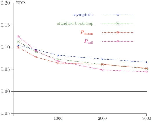
In Figure 15 ERPs are plotted for the testing procedures we have studied, at nominal level α = 0.05. These tests are, first, an asymptotic test based on the statistic (16) with critical values from the standard normal distribution, and then three bootstrap tests, the standard percentile-t bootstrap, the moon bootstrap, and the semiparametric
bootstrap. The hypothesis tested is that of equality of the indices TA and TB. For
distribution A, the data are drawn from the Singh-Maddala distribution (7) with the usual parameter values a = 100, b = 2.8, c = 1.7, while for distribution B, the par-ameters are a = 100, b = 4.8, c = 0.636659. The Theil index (2) has the same value for these two distributions. The tail indices are however quite different: for A it is 4.76, as previously noted, but for B it is 3.056, implying considerably heavier tails. For the largest sample sizes, the semiparametric bootstrap test is least distorted, although this is not so for smaller samples. All the tests except the asymptotic test are more distorted than those for which a specific value of the index is tested, probably because distribution B has a heavier tail than the distributions used for the other experiments. It may be remarked that, overall, the semiparametric bootstrap P value discrepancies are less than for the other tests, except for nominal levels between 0 and 10 percent.
Perhaps different choices of k and ptail would lead to better performance; we leave this
possibility for future work.
It is sometimes the case that the two samples are correlated, for instance if distributions A and B refer to pre-tax and post-tax incomes of a sample of individuals. In that case, resampling must be done in pairs, so that the correlation between the two incomes for the same individual are maintained in the bootstrap samples. In the case of paramet-ric estimation of the tail, a suitable parametparamet-ric method of imposing the appropriate correlation must be found, although we do not investigate this here.
Confidence Intervals
No simulation results on confidence intervals for inequality measures are presented in this paper, for two main reasons. The first is that little information would be conveyed by such results over and above that given by our results on ERPs if bootstrap confidence intervals are constructed in the usual manner, as follows. The chosen bootstrap method
gives a simulation-based estimate of the distribution of the bootstrap statistics W∗, of
which the quantiles can be used to construct confidence intervals of the form
[ ˆT − ˆσTc1−α/2, ˆT − ˆσTcα/2], (17)
for a confidence interval of nominal coverage 1− α. Here ˆσT = [ ˆV ( ˆT )]1/2, where ˆV ( ˆT ) is
given by (5), and c1−α/2 and cα/2 are the 1 − α/2 and α/2 quantiles of the distribution
of the W∗. One-sided confidence intervals can be constructed analogously.
The second reason is that the coverage errors of confidence intervals of the form (17) can converge to zero more slowly than the ERPs of bootstrap P values derived from the same bootstrap method. In order that a bootstrap confidence interval should be just as accurate as a bootstrap P value, a much more computationally intensive procedure should be used, whereby the interval is constructed by inverting the bootstrap test.
This means that the interval contains just those values T0 for which the hypothesis
T = T0 is not rejected by the bootstrap test. See Hansen(1999)for an example of this
method.
For these reasons, we prefer to defer to future work a study of the properties of bootstrap confidence intervals for inequality measures.
6. Poverty Measures
Cowell and Victoria-Feser (1996) show that poverty measures are robust to data
con-tamination of high incomes, if the poverty line is exogenous, or estimated as a function of the median or some other quantile, while inequality measures are not. This follows from the fact that poverty measures are not sensitive to the values of incomes above the poverty line. Consequently, we may expect that the standard bootstrap performs better with poverty measures than with inequality measures. In this section, we provide some Monte Carlo evidence on asymptotic and standard bootstrap inference for a poverty measure.
A popular class of poverty indices introduced by Foster, Greer, and Thorbecke (1984)
has the form
Pα= Z z 0 ³z − y z ´α dF (y) α ≥ 0,
where z is the poverty line. Let Yi, i = 1, . . . , n, be an IID sample from the
distribu-tion F . Consistent and asymptotically normal estimates of Pα and of its variance are
given respectively by ˆ Pα = 1 n n X i=1 ³z − Yi z ´α I(Yi ≤ z) and V ( ˆˆ Pα) = 1 n( ˆP2α− ˆP 2 α);
see Kakwani (1993). Thus in order to test the hypothesis that Pα = P0, for some given
value P0, we may use the following asymptotic t-type statistic:
Wp = ( ˆPα− P0)/[ ˆV ( ˆPα)]1/2,
We define the poverty line as half the median. For the Singh-Maddala distribution, the quantile function is
Q(p) =h(1 − p)
−1c − 1 a
i1b
from which we see that the poverty line is equal to z = Q(1/2)/2 = 0.075549 with our choice of parameters. In our simulations, we assume that this poverty line is known and we choose α = 2 rather than α = 1 as in the rest of the paper, because experimental
results of van Garderen and Schluter(2001)show that, with this choice, the distortion is
larger than with smaller values of α. The true population value of P2 can be computed
numerically: we obtain that P2 = 0.013016.
Figure 16 shows CDFs of the statistic Wp calculated from N = 10,000 samples drawn
from the Singh-Maddala distribution, for sample sizes n = 100, 500, 1,000, and 10,000.
We may compare the CDFs of Wpwith those of the statistic W for an inequality measure
(Figure 1). We see that, as expected, the discrepancy between the nominal N(0, 1) and the finite sample distributions of W decreases much faster in the former than in the latter case.
Figure 17 shows ERPs of asymptotic and standard bootstrap tests for sample sizes n = 100, 200, 500, and 1,000 for the FGT poverty measure with α = 2. We see that the ERP of the asymptotic test is quite large in small samples and is still significant in
large samples, but is less than that of Theil’s inequality measure inFigure 2. However,
the ERP of the bootstrap test is always close to zero for sample sizes greater than 100. Thus, as expected, we see that standard bootstrap methods perform very well with the FGT poverty measure, and give accurate inference in finite samples.
It may be wondered why we do not give results for sample sizes smaller than 100, as we did for the Theil index. The reason is just that, with smaller samples, there are moderately frequent draws, both from the Singh-Maddala distribution and from the bootstrap distributions, with no incomes below the poverty line at all. This makes it infeasible to perform inference on a poverty index for which the poverty line is around the 0.11 quantile of the distribution. On average, then, a sample of size 100 contains only 11 incomes below the poverty line; making the effective sample size very small indeed. Finally, the ERPs in the right-hand tail are, as expected, very small for all sample sizes considered.
7. Conclusion
In this paper, we have shown that asymptotic and standard bootstrap tests for the Theil inequality measure may not yield accurate inference, even if the sample size is very large. However bootstrap tests based on the FGT poverty measure perform very well as soon as sample sizes are large enough for there to be more than around 10 observations
below the poverty line. We find that the main reason for the dismal performance of the bootstrap with the inequality measure is the nature of the upper tail. This finding explains clearly why the bootstrap works badly for the inequality measure and works well for the poverty measure, which is unaffected by the upper tail of the distribution. Many parametric income distributions are heavy-tailed, by which it is meant that the upper tail decays like a power function. If the upper tail decays slowly enough, the variance can be infinite, in which case neither asymptotic nor bootstrap methods are consistent. In addition, even if the variance is finite, the frequent presence of extreme observations in sample data causes problems for the bootstrap.
To circumvent the problem caused by heavy tails, we studied the performance of a boot-strap method valid in the case of infinite variance: the m out of n or moon bootboot-strap. The direct results of this bootstrap are very sensitive to the subsample size m, and so we propose a method for exploiting this sensitivity in order to improve bootstrap reliability. This method yields a slight improvement over the standard bootstrap, but the error in the rejection probability is still significant with sample sizes up to and beyond 3,000. In another attempt to deal with the problem of heavy tails, we proposed a bootstrap that combines resampling of the main body of the distribution with a parametric boot-strap in the upper tail. This method gives dramatically improved performance over the standard bootstrap, with insignificant ERPs for sample sizes greater than around 1,000. Our simulation study is based on a specific choice of an inequality measure and of an income distribution. Additional experiments have been undertaken for different
inequality measures and different income distributions in Cowell and Flachaire(2004).
References
Abramowitz, M. and I. A. Stegun (1965). Handbook of Mathematical Functions. New-York: Dover.
Athreya, K. B. (1987). “Bootstrap of the mean in the infinite variance case”, Annals
of Statistics 15, 724–731.
Beran, R. (1988). “Prepivoting test statistics: a bootstrap view of asymptotic refinements”, Journal of the American Statistical Association 83 (403), 687–697. Bickel, P., F. G¨otze, and W. R. van Zwet (1997). “Resampling fewer than
n observations: gains, losses, and remedies for losses”, Statistica Sinica 7, 1–32.
Biewen, M. (2002). “Bootstrap inference for inequality, mobility and poverty measurement”, Journal of Econometrics 108, 317–342.
Brachman, K., A. Stich, and M. Trede (1996). “Evaluating parametric income distribution models”, Allgemeines Statistisches Archiv 80, 285–298.
Caers, J. and J. Van Dyck (1999). “Nonparametric tail estimation using a double bootstrap method”, Computational Statistics & Data Analysis 29, 191-211.
Coles, S. (2001). An Introduction to Statistical Modeling of Extreme Values. London: Springer.
Cowell, F. A. and E. Flachaire (2004). “Income distribution and inequality measurement: the problem of extreme values”, Working paper 2004.101, EUREQua, Universit´e Paris I Panth´eon-Sorbonne.
Cowell, F. A. and M.-P. Victoria-Feser (1996). “Poverty measurement with
contaminated data: a robust approach”, European Economic Review 40, 1761– 1771.
Davidson, R. and J.-Y. Duclos (1997). “Statistical inference for the measurement of the incidence of taxes and transfers”, Econometrica 65, 1453–1465.
Davidson, R. and J.-Y. Duclos (2000). “Statistical inference for stochastic dominance and for the measurement of poverty and inequality”, Econometrica 68, 1435–1464. Davidson, R. and J. G. MacKinnon (1993). Estimation and Inference in
Econometrics. New York: Oxford University Press.
Davidson, R. and J. G. MacKinnon (1998). “Graphical Methods for Investigating the Size and Power of Hypothesis Tests”, The Manchester School 66, 1–26.
Davidson, R. and J. G. MacKinnon (1999). “The size distortion of bootstrap tests”, Econometric Theory 15, 361–376.
Foster, J. E., J. Greer, and E. Thorbecke (1984). “A class of decomposable poverty measures”, Econometrica 52, 761–776.
Gilleland, E. and R. W. Katz (2005). Extremes Toolkit: Weather and Climate Applications of Extreme Value Statistics. R software and accompanying tutorial. Hall, P. (1990). “Asymptotic properties of the bootstrap for heavy-tailed
distributions”, Annals of Probability 18, 1342–1360.
Hall, P. (1992). The Bootstrap and Edgeworth Expansion. Springer Series in Statistics. New York: Springer Verlag.
Hall, P. and Q. Yao (2003). “Inference in arch and garch models with heavy-tailed errors”, Econometrica 71, 285–318.
Hampel, F. R., E. M. Ronchetti, P. J. Rousseeuw, and W. A. Stahel (1986). Robust Statistics: The Approach Based On Influence Functions. New-York: Wiley.
Hansen, B. E., (1999). “The grid bootstrap and the autoregressive model”, Review of Economics and Statistics 81, 594–607.
Hill, B. M. (1975). “A Simple General Approach to Inference about the Tail of a Distribution”, Annals of Statistics 3, 1163–1174.
Horowitz, J. L. (2000). “The Bootstrap”, in Handbook of Econometrics, Volume 5. J. J. Heckman and E. E. Leamer (eds), Elsevier Science.
Huber, P. J. (1981). Robust Statistics. New-York: Wiley.
Kakwani, N. (1993). “Statistical inference in the measurement of poverty”, Review of
Economics and Statistics 75, 632–639.
Knight, K. (1989). “On the bootstrap of the sample mean in the infinite variance case”, Annals of Statistics 17, 1168–1175.
Maasoumi, E. (1997). “Empirical analyses of inequality and welfare”, in Handbook
of Applied Econometrics : Microeconomics, pp 202–245. M. H. Pesaran and
P. Schmidt (eds), Blackwell.
Mills, J. and S. Zandvakili (1997). “Statistical inference via bootstrapping for measures of inequality”, Journal of Applied Econometrics 12, 133–150. Politis, D. N. and J. P. Romano (1994). “The stationary bootstrap”, Journal of
American Statistical Association 89, 1303–13013.
Schluter, C. and M. Trede (2002). “Tails of Lorenz curves”, Journal of
Econometrics 109, 151–166.
Tukey, J. W. (1977). Exploratory Data Analysis. Reading: Addison-Wesley. van Garderen, K. J. and C. Schluter (2001). “Improving finite sample confidence
Table 1
min q1 median q3 max
ˆ
V( ˆT) 0.005748 0.026318 0.034292 0.045562 0.264562 ˆ
V′( ˆT) 0.005334 0.024297 0.031355 0.040187 0.119723
Minimum, maximum, and quartiles of 10,000 realizations of ˆV( ˆT) and ˆV′( ˆT).
Table 2
asymptotic std bootstrap Pmoon Ptail
b= 2.1, c = 1 0.41 0.24 0.15 0.16
-0.03 -0.04 -0.03 0.04
b= 1.9, c = 1 0.48 0.28 0.20 0.18
-0.03 -0.04 -0.02 0.06
−3 −2 −1 0 1 2 3 0.0 0.1 0.2 0.3 0.4 0.5 0.6 0.7 0.8 0.9 1.0 ... ... ... ... ... ... ... ... ... ... ... ... ... ... ... ... ... ... ... ... ... ... ... ... ... ... ... ... ... ... ... ... ... ... ... ... ... n = 20 ... ... ... ... ... ... ... ... ... ... ... ... ... ... ... ... ... ... ... ... ... ... ... ... ... ... ... ... ... ... ... ... ... ... ... ... ... ... ... ... ... ... ... ... ... n = 50 ... ... ... ... ... ... ... ... ... ... ... ... ... ... ... ... ... ... ... ... ... ... ... ... ... ... ... ... ... ... ... ... ... ... ... ... ... ... ... n = 100 ... ... ... ... ... ... ... ... ... ... ... ... ... ... ... ... ... ... ... ... ... ... ... ... ... ... ... ... ... ... ... ... ... ... ... ... ... ... n = 1000 ... ... ... ... ... ... ... ... ... ... ... ... ... ... ... ... ... ... ... ... ... ... ... ... ... ... ... ... ... ... ... ... n = 10000 ... ... ... ... ... ... ... ... ... ... ... ... ... ... ... ... ... ... ... ... ... ... ... ... ... ... ... ... ... ... ... N(0, 1) w F (w)
0.00 0.02 0.04 0.06 0.08 0.10 0.12 0.14 0.16 0.18 0.20 ... ... ... ... ... ... ... ... ... ... ... ... ... ... ... ... ... ... ... ... ... ... ... ... ... ... ... ... ... ... ... ... ... ... ... ... ...... ...... ... ...... ...... ...... ⋆ ⋆ ⋆ ⋆ ⋆ ⋆ ⋆ ⋆ ⋆ ...⋆ asymptotic ...... ...... ...... ... ...... ... ...... ...... ... ××× × × × × × × ...× percentile-t ... ... ... ... ... ... ... ... ... ... ... ... ... ... ... ... ... ... ... ... ... ... ... ... ... ... ... ... ... ... ... ... ... ... ... ... ... ...... ... ... ... ... ...... ...... ...... ...... ◦ ◦ ◦ ◦ ◦ ◦ ◦ ◦ ◦ ...◦ percentile ... ... ... ... ... ... ... ... ... ... ...... ... ... ... ...... ... ... ... ...... ... ...... ...... ...... ...... ⋄ ⋄ ⋄ ⋄ ⋄ ⋄ ⋄ ⋄ ⋄ ...⋄ bias corrected n ERP 1000 2000 3000 4000 5000
−0.05 −0.03 −0.01 0.01 0.03 0.05 ... ... ... ... ... ⋆⋆⋆ ⋆ ⋆ ⋆ ⋆ ⋆ ⋆ ...⋆ asymptotic ... ... ... ... ... ××× × × × × × × ...⋆ percentile t ... ... ... ... ......... ... .. ◦ ◦ ◦ ◦ ◦ ◦ ◦ ◦ ◦ ...◦ percentile ... ... ... ... ... ... ... ... ... ...... ... ...... ... ...... ... ⋄ ⋄ ⋄ ⋄ ⋄ ⋄ ⋄ ⋄ ⋄ ...⋆ bias corrected n ERP 1000 2000 3000 4000 5000 ...
Figure 3. ERPs in right-hand tail
−3 −2 −1 0 1 2 3 0.0 0.1 0.2 0.3 0.4 0.5 0.6 0.7 0.8 0.9 1.0 ... ... ... ... ... ... ... ... ... ... ... ... ... ... ... ... ... ... ... ... ... ... ... ... ... ... w1 ... ... ... ... ... ... ... ... ... ... ... ... ... ... ... ... ... ... ... ... ... ... ... ... ... ... ... ... ... ... ... ... ... w2 ... ... ... ... ... ... ... ... ... ... ... ... ... ... ... ... ... ... ... ... ... ... ... w3 ... ... ... ... ... ... ... ... ... ... ... ... ... ... ... ... ... ... ... ... ... ... ... W ... ... ... ... ... ... ... ... ... ... ... ... ... ... ... ... ... ... ... ... ... ... ... N(0, 1) w F (w) Figure 4. CDFs of w1, w2, w3, and W , n= 20
−3 −2 −1 0 1 2 3 0.0 0.1 0.2 0.3 0.4 0.5 0.6 0.7 0.8 0.9 1.0 ... ... ... ... ... ... ... ... ... ... ... ... ... ... ... ... ... ... ... ... ... ... ... ... W ... ... ... ... ... ... ... ... ... ... ... ... ... ... ... ... ... ... ... ... ... ... W′ ... ... ... ... ... ... ... ... ... ... ... ... ... ... ... ... ... ... ... ... ... ... ... ... ... ... ... ... ... ... N(0, 1) w F (w) Figure 5. CDFs of W and W′, n = 20 −3 −2 −1 0 1 2 3 0.0 0.1 0.2 0.3 0.4 0.5 0.6 0.7 0.8 0.9 1.0 ... ... ... ... ... ... ... ... ... ... ... ... ... ... ... ... ... ... ... ... ... ... ... ... ... ... n = 20 ... ... ... ... ... ... ... ... ... ... ... ... ... ... ... ... ... ... ... ... ... ... ... ... ... ... ... ... ... ... ... ... n = 50 ... ... ... ... ... ... ... ... ... ... ... ... ... ... ... ... ... ... ... ... ... ... ... ... ... ... ... n = 100 ... ... ... ... ... ... ... ... ... ... ... ... ... ... ... ... ... ... ... ... ... ... ... ... ... ... ... n = 1000 ... ... ... ... ... ... ... ... ... ... ... ... ... ... ... ... ... ... ... ... ... ... ... ... ... ... ... ... ... N(0, 1) w F (w)
0.00 0.02 0.04 0.06 0.08 0.10 0.12 ... ... ... ... ... ... ... ... ... ... ... ... ... ... ... ... ... ... ... ... ... ... ...... ...... ...... ...... ...... ...... ⋆ ⋆ ⋆ ⋆ ⋆ ⋆ ⋆ ...⋆ asymptotic ... ... ... ......... × × × × × × × ...× percentile-t n ERP 1000 2000 3000
Figure 7. ERPs with truncated Singh-Maddala
−0.06 −0.04 −0.02 0.00 0.02 0.04 0.06 ⋆⋆⋆⋆⋆⋆⋆ ⋆⋆ ⋆⋆ ⋆⋆⋆ ⋆⋆ ⋆⋆⋆ ⋆⋆⋆ ⋆⋆⋆ ⋆⋆⋆⋆⋆⋆ ⋆⋆⋆⋆⋆⋆ ⋆⋆⋆⋆⋆⋆⋆⋆⋆ ⋆⋆⋆ ... m ERP 5 10 15 20 25 30 35 40 45 50
0.0 0.1 0.2 0.3 0.4 0.5 0.6 0.7 0.0 0.1 0.2 0.3 0.4 0.5 0.6 0.7 ...... ... ... ... ... .... .... .... .... .... .... .... .... ... ... ... ... ... ... ... ... .... .... .... .... .... ... ... ... ... ... ... ... ... ... ... ... ... ... ... ... ... ... ... ... ... ... ... ... ... ... ... ... ... ... ... ... ... ... ... ... ... ... ... ... ... ... ... ... ... ... ... ... ... ... ... ... ... ... ... ... ... ... ... ... ... ... ... ... ... ... ... ... ... ... ... ... ... ... ... ... ... ... ... ... ... ... ... ... ... ... ... ... ... ... ... ... ... ... ... ... ... ... ... ... ... .... .... .... .... .... .... .... .... .... .... .... .... .... .... .... .... .... .... .... .... .... .... .... . n = 50 m−1/2 P value 0.0 0.1 0.2 0.3 0.4 0.5 0.6 0.7 0.2 0.3 0.4 0.5 0.6 0.7 0.8 0.9 ......... ... ... ... ... .... .... ... .... .... ... .... ... .... .... .... .... .... .... ... ... ... ... ... ... ... ... ... ... ... ... ... ... ... .... .... ... ... ... ... ... ... ... ... ... ... ... ... ... ... ... ... ... ... ... ... ... ... ... ... ... ... ... ... ... ... ... ... ... ... ... ... ... ... ... ... ... ... ... ... ... ... ... ... ... ... ... ... ... ... ... ... ... ... ... ... ... ... ... ... ... ... ... ... ... ... ... ... ... ... ... ... ... ... ... ... ... ... ... ... ... ... ... ... ... ... ... ... ... ... ... ... ... ... ... ... ... ... ... ... ... ... ... ... ... ... ... ... ... ... ... ... ... ... ... ... ... ... ... ... ... ... ... ... ... n = 500 m−1/2 P value
Figure 9. Sample paths of the moon bootstrap P value as a function of m
5 10 15 20 25 0.10 0.15 0.20 0.25 0.30 ... ...... ...... ...... ... ... ... ... ... ...... ...... ... ... ... ... ...... ... ... ... ... n = 50 m Pmoon 50 100 150 200 250 0.50 0.55 0.60 0.65 0.70 .................. ... ...... ...... ... ... ........................ ......... ... ... ... ... ...... ... ... ... ... ... ...... ... ...... ... ... ... ... ... ... ... ...... ...... ......... ... ... ... ...... ...... ... ......... ... ... ... ...... ... ... ... ... ... ... ...... ...... ... ...... ... ... ... ... ... ... ... ... ... ... ...... ...... ......... ... ... ... ... ......... ...... ......... ... ... ... ... ...... ... ... ... ... ... ... ... ... ... ... ...... ... ... ... ...... ... ... ... ... ... ... ... ... ...... ... ... ... ... ... ... ... ... ... ... ... ... ... ... ... ... ... ... ... ...... ... ... ... ... ...... ... ... ... ... ... ... ... ......... ... ... ... ... ... ... ... ... ... ...... ... ... ... ... ... ... ...... ... ...... ...... ... n = 500 m Pmoon
−0.05 0.00 0.05 0.10 0.15 0.20 ... ... ... ... ... ... ... ... ... ... ... ... ...... ...... ...... ...... ... ...... ... ...... ... ⋆ ⋆ ⋆ ⋆ ⋆ ⋆ ⋆ ...⋆ asymptotic ...... ...... ...... ××× × × × × ...× standard bootstrap ... ... ... ... ... ... ... ... ... ◦◦ ◦ ◦ ◦ ◦ ◦ ...◦ Pmoon ... ... ... ... ... ... ... ... ... ... ...... ... ... ⋄ ⋄ ⋄ ⋄ ⋄ ⋄ ⋄ ...⋄ Ptail n ERP 1000 2000 3000 ...
Figure 11. Comparison of ERPs in left-hand tail
−0.05 0.00 0.05 ... ... ... ⋆⋆⋆ ⋆ ⋆ ⋆ ⋆ ...⋆ asymptotic ... ... ... ... ××× × × × × ...× standard bootstrap ... ... ◦◦◦ ◦ ◦ ◦ ◦ ...◦ Pmoon ... ... ... ... ... ... ............ ... ⋄ ⋄⋄ ⋄ ⋄ ⋄ ⋄ ...⋄ Ptail n ERP 1000 2000 3000 ...
0.0 0.1 0.2 0.3 0.4 0.5 0.6 0.7 0.8 0.9 1.0 −0.05 0.00 0.05 0.10 0.15 ... ... ... ... ... ... ... ... ... ... ... ... ... ... ... ...... ... ...... ...... ... ...... ...... ...... ... ... ... ... asymptotic ... ... ... ... ... ...... ...... ....... ... standard bootstrap ... ... ...... ... ......... . ... Ptail ...... ... ... ... ... ... ... ... ... ... ...... ......... ...... ...... ...... ... Pmoon ... x F (x) − x
Figure 13. P value discrepancy plots
0.0 0.1 0.2 0.3 0.4 0.5 0.6 0.7 0.8 0.9 1.0 −0.05 0.00 0.05 0.10 ... ...... ...... ...... ...... ... ... .... ... h= 0.3 ... ... ...... ... ......... ... ... h= 0.4 ... ...... ......... ... . ... h= 0.6 ...... ...... ...... ... ... ... ... ... h= 0.8 ...... ...... ...... ... ... ... ... ... h= 1.0 ... x F (x) − x