HAL Id: hal-00941532
https://hal.inria.fr/hal-00941532
Submitted on 31 Mar 2016
HAL is a multi-disciplinary open access
archive for the deposit and dissemination of
sci-entific research documents, whether they are
pub-lished or not. The documents may come from
teaching and research institutions in France or
L’archive ouverte pluridisciplinaire HAL, est
destinée au dépôt et à la diffusion de documents
scientifiques de niveau recherche, publiés ou non,
émanant des établissements d’enseignement et de
recherche français ou étrangers, des laboratoires
Power Consumption Models for the Use of Dynamic and
Partial Reconfiguration
Robin Bonamy, Sebastien Bilavarn, Daniel Chillet, Olivier Sentieys
To cite this version:
Robin Bonamy, Sebastien Bilavarn, Daniel Chillet, Olivier Sentieys. Power Consumption Models for
the Use of Dynamic and Partial Reconfiguration. Microprocessors and Microsystems: Embedded
Hardware Design (MICPRO), Elsevier, 2014, �10.1016/j.micpro.2014.01.002�. �hal-00941532�
Power Consumption Models for the Use of
Dynamic and Partial Reconfiguration
Robin Bonamy
S´
ebastien Bilavarn
Daniel Chillet
Olivier Sentieys
Abstract
Minimizing the energy consumption and silicon area are usually two major challenges in the design of battery-powered embedded computing systems. Dynamic and Partial Reconfiguration (DPR) opens up promis-ing prospects with the ability to reduce jointly performance and area of compute-intensive functions. However, partial reconfiguration manage-ment involves complex interactions making energy benefits very difficult to analyze. In particular, it is essential to realistically quantify the energy loss since the reconfiguration process itself introduces overheads. This paper addresses this topic and presents a detailed investigation of the power and energy costs associated to the different operations involved with the DPR capability. From actual measurements considering a Xil-inx ICAP reconfiguration controller, results highlight other components involved in DPR power consumption, and lead to the proposition of three power models of different complexity and accuracy tradeoffs. Addition-ally, we illustrate the exploitation of these models to improve the analysis of DPR energy benefits in a realistic application example.
1
Introduction
Run-time reconfiguration, i.e. the ability to modify hardware execution re-sources to ensure specific functions arrangement during execution, has been a promising field of research since the 1990s [Lemoine and Merceron(1995)]. The technology, now referred to as Dynamic and Partial Reconfiguration (DPR), is fully operational and available in up to date devices from the two major FPGA manufacturers, Xilinx and Altera. Run-time reconfiguration allows sharing a piece of silicon area for the implementation of different hardware accelerators when tasks are sequentially executed. This results in significantly less FPGA resources for reconfigurable processing.
Whereas many tools are available for the actual management and program-ming of DPR functionalities, there are comparatively few methodologies helping to explore and evaluate these benefits. However, the costs of reconfiguration and hardware implementation of tasks involve complex issues that need to be well understood to determine whether or not the gains exceed the costs. Considering
for example an application as a set of tasks with possible hardware implemen-tations, different execution scenarios will influence the actual performance, area and energy tradeoff of a solution: i) use static hardware tasks, ii) use dynamic hardware tasks and reconfigure when necessary, iii) use software tasks and iv) use a mix of software and hardware tasks, possibly statically or dynamically con-figurable, possibly at different cost-performance tradeoffs for hardware tasks. In order to assess this very large opportunity of choices, fast and accurate mod-els of DPR reconfiguration must be defined, especially in terms of power and energy. This paper addresses this problem and investigates the definition, devel-opment and use of such models that can be able firstly, to explore combinations of task implementations, and secondly to provide the associated schedule that will allow minimizing the energy consumption. Therefore, providing reliable power models is the main contribution of this work which is based on actual experimentation of the DPR process in Xilinx devices. Fine measurements on a Virtex5 FPGA have led to define three models of different accuracy/complexity tradeoffs. Additionally, we also address an application study of the proposed models on a representative real life example to show their usefulness in early design space exploration for energy efficiency.
The outline of the paper is the following. First, we present the context of this work with a state of the art on power consumption related to the DPR ability, an introduction to FPGA architectural features for DPR and the experimental setup developed for accurate power measurements. Extensive measurement re-sults are then analyzed in detail in section III, and exploited in section IV to define different models for power estimation that are further validated in section V. The following section VI proposes a case study of these models in the design space exploration of a HW/SW implementation of a H.264/AVC profile video decoder application. Finally, section VII summarizes the main conclusions and presents next directions of research.
2
Work Context
2.1
State of The Art
DPR is a technique enabled in reconfigurable hardware devices like FPGAs to improve their processing flexibility. Indeed their configuration can be changed
during execution according to user constraints or environmental needs [Tadigotla et al.(2006)Tadigotla, Sliger, and Commuri]. This run-time tasks configuration ability comes with various opportunities for
energy saving. First, dedicated hardware allows the definition of optimal imple-mentations in terms of processing and energy efficiency. DPR can then be widely used to increase the resource usage [Eldredge and Hutchings(1996)], further re-ducing the size of reconfigurable units and the associated static power consump-tion. Dynamic reconfiguration also lets the modification of clock configuration, i.e. it provides dynamic frequency adaptation and variation of performances, to
adjust power consumption and energy efficiency on demand [Zhang et al.(2008)Zhang, Rabah, and Weber]. In addition, DPR can also be used to disable the routing of clock signals to some
of the FPGA resources, thus to implement a low overhead clock gating technique
with interesting results [Sterpone et al.(2011)Sterpone, Carro, Matos, Wong, and Fakhar]. An important drawback of DPR in most applications is the unavailability of
the region involved during the reconfiguration process. Limiting the reconfigura-tion time is thus a critical requirement that can be addressed with different tech-niques. A first one is to improve the reconfiguration speed to reach the maximum
reconfiguration port throughput [Claus et al.(2008)Claus, Zhang, Stechele, Braun, Hubner, and Becker]. For example, using higher performance memory for bitstream storage (DDR)
and DMA can greatly reduce memory access times to the bitstream. Another solution is to reduce the size of the configuration data, based for instance on coding only the differences with previous configuration instead of the completely new configuration information. In any case, the overhead of reconfigurations is important to consider in the design process. This has been shown in many recent
works [Rullmann and Merker(2008), Duhem et al.(2012)Duhem, Muller, and Lorenzini], but reconfiguration delays are not the only issue. The energy cost of DPR is also
an important design parameter to manage, especially to ensure actual energy gains from its utilization. We can find a few studies on the power consumption of
dynamic reconfiguration in the literature like [Becker et al.(2003)Becker, Huebner, and Ullmann], [Lorenz et al.(2004)Lorenz, Mengibar, Valderas, and Entrena] and more recently
[Bonamy et al.(2012)Bonamy, Pham, Pillement, and Chillet]. These works gen-erally address the reconfiguration controller and throughput optimization but do not provide a thorough analysis and modeling of power consumption during partial reconfiguration.
The fine investigation of power and energy consumption and modeling dur-ing DPR is the main focus of this paper. This contribution is part of a more global design space exploration methodology developed in the context of a plat-form project focusing on power measurement, estimation and optimization for heterogeneous hardware-software computing systems [ope(2013)]. In the fol-lowing, we detail the elaboration of power estimations at different accuracy and complexity tradeoffs from actual and fine power measurements. We also show the applicability and usefulness of the proposed models in adapting the level of estimation complexity to the best suited accuracy imposed by the ap-plication analysis. It is then demonstrated how these models greatly help the analysis of difficult implementation choices including static hardware tasks, soft-ware execution and dynamic reconfiguration using the design space exploration methodology mentioned previously.
2.2
FPGA Architecture and Partial Reconfiguration
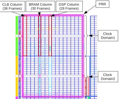
Effective DPR is available in Xilinx FPGAs since the VirtexII pro series and more recently in Altera Stratix V devices. This work is based on Xilinx technol-ogy and targets more specifically the Virtex5 XC5VLX50T device of a ML550 Evaluation platform for power measurement reasons. A view of the correspond-ing layout is presented in figure 1. This FPGA is organized in six clock do-mains where each clock domain is composed of several frames. These frames are grouped in columns containing either CLBs (slices), DSPs, BRAMs or other
CLB Column
(36 Frames) BRAM Column(30 Frames) DSP Column(28 Frames)
Clock Domain1 PRR
Clock Domain2
Figure 1: Top left hand of Virtex-5 XC5VLX50T FPGA layout (Xilinx PlanA-head 12.1).
specific blocks. The number of frames in one column is fixed by the FPGA architecture and is dependent on the type of these columns. The minimum ad-dressable reconfiguration area is a frame whose configuration requires 41 words of 4 bytes (164 bytes). The minimum recommended reconfiguration area is a column, so a Partial Reconfigurable Region (PRR) must be a multiple of the number of frames and mainly contains CLBs, DSPs and BRAMs.
Figure 2 represents the organization of the configuration file (bitstream) to configure the PRR example of figure 1. The first few words represent the header containing information on the bitstream and configuration startup procedure. The next word is the address of the first frame to configure, followed by the configuration words for the CLB frames. After four CLB columns comes the successive configuration of a BRAM column, two CLB columns and a DSP column. The configuration of this first clock domain ends with CLB data up to the right bound of the PRR. The second clock domain starts with another frame address corresponding to the first column and follows the same column pattern (CLB, BRAM, CLB, DSP). Finally the BRAM content is addressed and a few additional words end the configuration file.
2.3
Experimental Setup
2.3.1 Power Measurement
A Virtex-5 LXT ML550 Networking Interface & Power Measurement Platform [ML5(2013)] is used in the following experiments. The choice of this platform
Bitstream header Frame address CLB Frames configuration Frame address BRAM content configuration End of configuration BRAM Frames configuration CLB Frames configuration DSP Frames configuration CLB Frames configuration Frame address CLB Frames configuration BRAM Frames configuration CLB Frames configuration DSP Frames configuration CLB Frames configuration Frame address BRAM content configuration 1st clock domain 2nd clock domain BRAM data
B its re am fi le c o nt en t
Figure 2: Bitstream composition to configure a PRR (Xilinx ISE 12.1).
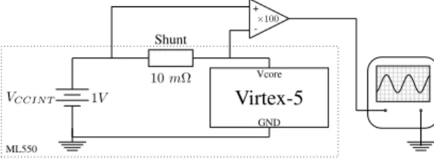
1V VCCIN T Shunt 10 mΩ Virtex-5 Vcore GND ML550 + -×100
Figure 3: Power measurement procedure using a ML550 platform, high-precision amplifier and digital oscilloscope.
was motivated by the availability of built-in resources that greatly helps ana-lyzing power consumption. Indeed five connectors are present on the board to access the currents consumed by the FPGA and its peripherals. FPGA power measurement is based on monitoring the power rail of the core. As represented in figure 3, a high-precision amplifier is used to improve the signal level which is then sent to a digital oscilloscope. With this procedure, it is possible to measure power values as low as 0.1mW . As it will be shown, this precision is sufficient to clearly identify the different steps of a dynamic reconfiguration process and derive accurate power models.
2.3.2 Platform Setup
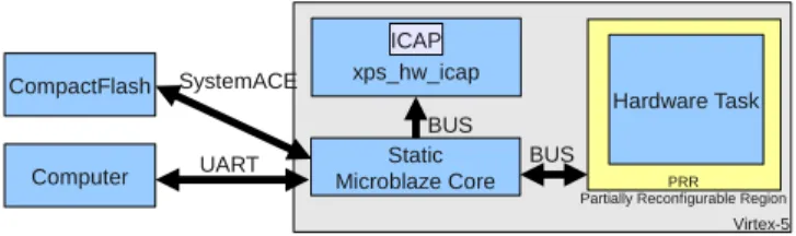
The ML550 platform is configured using the Xilinx Reference Design described in [Xilinx(2011)]. The system is composed of a MicroBlaze processor, a Compact-Flash memory controller and a xps_hw_icap reconfiguration controller, as shown in figure 4. The MicroBlaze processor and the reconfiguration controller oper-ate both at 100M Hz. Reconfiguration requests are managed by the MicroBlaze
Static Microblaze Core
Hardware Task
Computer UART BUS
xps_hw_icap
CompactFlash SystemACE
BUS
PRR Partially Reconfigurable Region
ICAP
Virtex-5
Figure 4: Reference Design used during measurement procedure.
Table 1: FPGA Resources and idle power of tasks used for measurements.
Task BRAMs Slices DSPs Idle power(mW )
T1 8 169 2 26
T2 8 154 1 24
Tblank 0 0 0 0
FPGA without task 402
which reads a configuration bitstream from the CompactFlash and sends it to the xps_hw_icap to apply the corresponding configuration to a PRR.
Since different tasks are used in the following experiments, one PRR fitting the area of the biggest task is defined. We selected a PRR that holds in the top left hand of the FPGA layout as shown in figure 1, and occupies the com-plete area over two clock domains. Doing this corresponds to a configuration bitstream with a fixed size of 227700 Bytes. During a measurement process, the FPGA core is powered at 1V and we make sure that the die temperature keeps stable around 35◦C in order to focus on power consumption variations only due to the DPR. As it is visible for example in figure 5, we can clearly detect the distinct phases of the reconfiguration process thanks to this procedure.
2.3.3 PRR and Tasks
Power measurements are made using previous PRR that can be configured with three different tasks. The first task T1 is a matrix multiplication. The second
task T2 is a parallel version of the matrix multiplication. The two RTL
imple-mentations of the matrix multiplication are derived from High Level Synthesis
with different loop unrolling settings [Bonamy et al.(2011)Bonamy, Chillet, Sentieys, and Bilavarn]. They correspond to a sequential and a parallel solution which FPGA resources
are given in table 1. The third task is called a blank bitstream and will be referred to as Tblank in the following. A blank bitstream corresponds to the
configuration of an empty PRR. This is useful to clear the configuration of a PRR when it is unused and thus to reduce the associated power consumption [Liu et al.(2010)Liu, Pittman, and Forin]. In the following, we analyze in de-tail how configuring from one task to another impacts the FPGA core power consumption.
3
Power Consumption Analysis
The overall DPR process consists mainly in transferring data to the differ-ent compondiffer-ents involved (CompactFlash, MicroBlaze local BRAM memory, xps_hw_icap reconfiguration controller and configuration memory). The full procedure can be split into the following basic steps. The configuration data are successively:
• loaded from a file stored on the CompactFlash and buffered to the MicroBlaze local memory.
• written from the Microblaze local memory to the xps_hw_icap reconfig-uration controller.
• written from the xps_hw_icap to the Internal Configuration Access Port (ICAP).
• written from the ICAP to the configuration memory.
• applied from the configuration memory to the configurable resources (CLB, BRAM, DSP, interconnect).
Under these circumstances, the global reconfiguration power is the result of a combination of two main elements: i) reconfiguration control involving mainly configuration data accesses and ii) the actual configuration of the FPGA resources.
3.1
Configuration Data Access
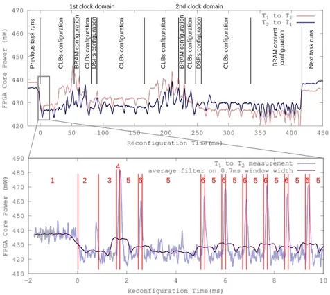
Top of figure 5 reports the power profiles of the FPGA core during DPR from T2
to T1(black), and from T1to T2(gray). If we inspect closely the full
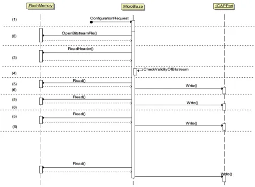
reconfigura-tion process in this figure, we can observe the power variareconfigura-tions due to the DPR procedure. The bottom plot of figure 5 is a zoom on the first 10ms of DPR. To provide even finer power analysis, we have introduced software triggered mark-ers in the reconfiguration control to highlight each step of the process. Seven steps are thus clearly identified and presented in the sequence diagram of figure 6:
1. receive reconfiguration order
2. open bitstream file on the CompactFlash 3. read bitstream file header
4. check validity of bitstream file header
5. read file fragment on the CompactFlash 6. write data in xps_hw_icap
1 2 3 5 4 5 6 6 5 6 5 6 5 6 5 6 5 6 5 P rev iou s ta sk ru ns CLBs co nfi gu ratio n BRAM con fig ura tio n C L Bs co nfig ura tio n DSPs conf igu rati on CLBs co nfi gu ratio n CLB s co nfig urat io n BRAM co nfig ura tio n CLBs con fig urat ion DSPs conf ig urati on CLBs confi gu rati on BRAM con tent co nfi gu ratio n Nex t tas k runs
1st clock domain 2nd clock domain
Figure 5: Top plot is the FPGA core power consumption during DPR from T2
to T1(black) and from T1 to T2 (gray). Bitstream composition is scaled to the
reconfiguration time to outline the reconfiguration steps. Bottom plot is a zoom on the first 10ms of DPR.
We can notice that the lowest levels in the power profile of figure 5 (bottom plot) correspond to read accesses to the CompactFlash (phases 3 and 5). Due to the relative slowness of the CompactFlash, the MicroBlaze processor (which has the largest part of FPGA power) is mostly waiting for data during these accesses and does not generate a lot of activity. However writing implies much more work (phase 6) involving bus traffic, reconfiguration controller activity and FPGA resources configuration. The corresponding power overheads are about 45mW which is more than 10% of the overall FPGA power consumption. There is another power overhead during bitstream validity check (phase 4). This overconsumption is also significant as it is processed by the MicroBlaze processor. Note that these power peaks are not visible on top of figure 5 because of an average filtering scheme used for display convenience. Finally reading file fragments and writing configuration data to the xps_hw_icap are repeated up to the end of the bitstream.
Figure 6: Sequence diagram of the reconfiguration process.
3.2
Configuration Application
Previous zoom highlighted the influence of configuration data transfers on power consumption. Nevertheless, the effects of these read and write operations should not bring significant variations on global power profiles (top of figure 5). Indeed, if we compute an average sliding window over 0.7ms (black curve, bottom of figure 5), the resulting profile is very regular and not far from constant. How-ever, global power profiles are clearly not constant over the full duration of the reconfiguration process. Firstly, two power overconsumptions located around 50 and 200ms are present and look like two “waves”. Secondly, power levels at the beginning and at the end of the reconfiguration are different. This power difference seems to be related to the transition from previous to the next task. These two effects indicate that power profiles also depend on other parame-ters than configuration data accesses. We assume that the observed power vari-ations are also due to the bitstream contents and we separate two kind of effects: power surges and power steps. A reconfiguration can cause overconsumptions due to the activity resulting from differences with previous configuration (power surges). Then, configuration application enables or disables signals and blocks that can cause power consumption breaks (power steps). The following sections detail the analysis of power profiles that justifies these assumptions.
3.2.1 Power Surges
In the power profiles of figure 5 showing the reconfiguration of T2 from T1
(gray) and T1from T2(black), both curves have the same overall shape which is
mainly driven by the write operation in the reconfiguration memory. Practically, when a task is configured over a previous task, reconfiguration consists in re-writing data on the existing content of the configuration memory. If both nth
words in the bitstreams of previous and next tasks are the same, the memory cells don’t change and the power consumption is low. Inversely, if the two words in the bitstreams are exactly complementary, each bit of the memory cell changes and this leads to a larger power consumption. From this observation, we assume that power consumption during the reconfiguration process is linked to the differences between the bitstreams of previous and next task configurations. These differences can be quantified by a metric like the Hamming distance.
On both curves of figure 5, two remarkable zones are present: the first one is located around 50ms and the second one around 200ms. The amplitude of these overconsumptions is about 15mW . Further analysis of the bitstream con-tent shows that these two zones correspond to the configuration of two BRAM frames. The BRAM frames belong in two distinct clock domains which explains the presence of two overconsumption zones. By correlating this information with the design view of Xilinx floorplanning tool (PlanAhead), we can notice that the density of slices is higher close to the BRAM frames. This placement of logic resources around the BRAM blocks can be explained by the Place and Route algorithms which probably try to group the resources to limit the cost of interconnections.
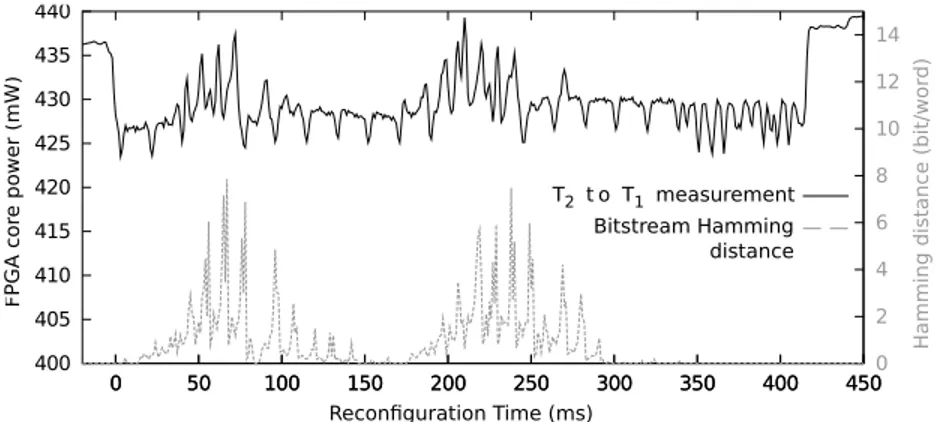
Top of figure 7 shows the power profile of the PRR reconfiguration from T1to
T2. Bottom of this figure shows the Hamming distance per configuration word of
32-bit between the two corresponding bitstreams. Abscissa values are adjusted to tie in the reconfiguration time (ms). We can notice on these curves that the shape of the Hamming distance is highly correlated to the shape of the power consumption profile. The Hamming distance peaks at the same time when the overconsumptions are present, around 50ms and 200 − 250ms. This tends to confirm the link between configuration differences and overconsumption values (power surges).
These results suggest that overconsumptions result from differences between previous and next configurations, which in turn correspond to the activation and deactivation of interconnects between FPGA resources. This may cause un-wanted connections and perhaps small short circuits while the PRR is not fully
configured, as suggested by [Lorenz et al.(2004)Lorenz, Mengibar, Valderas, and Entrena] for an ATMEL device. Modifications of the FPGA interconnect are indicated
in the bitstream and reflected in the Hamming distance.
3.2.2 Power Steps
Looking more closely at figure 5 reveals that the power levels at the beginning and the end of the reconfiguration are different. This difference is coherent
400 405 410 415 420 425 430 435 440 0 50 100 150 200 250 300 350 400 450 FPGA c or e po wer (mW ) 0 50 100 150 200 250 300 350 400 4500 2 4 6 8 10 12 14 Hammi ng d ista nce ( bit/w or d) Reconfiguration Time (ms) T2 t o T1 measurement Bitstream Hamming distance
Figure 7: Power consumption during DPR from T2 to T1 (straight black line)
and Hamming distance per configuration word of 32-bit in T2and T1bitstreams
(dashed gray plot).
with the power consumption of tasks presented in table 1 where the global power is 402mW for an empty FPGA, and 428mW or 426mW respectively when tasks T1 or T2 are configured. T1 and T2 don’t have the same idle power
consumption which depends on their size. Logically, using two tasks with more idle power differences should emphasize this observation. As an illustration, figure 8 presents the power profile during the partial dynamic reconfiguration of a PRR from Tblank to T2, where Tblank is an empty or blank task as defined
previously. This figure explicitly shows two power steps at 55ms and 220ms. These steps raise progressively the power level from the idle power of previous task Tblank to the idle power of next task T2. Figure 8 also highlights the
corresponding bitstream composition of the Virtex5 device which reveals that two steps appear just before the configuration of BRAMs. This behavior is typical of activating or deactivating elements and suggests that there is probably a link with the power consumption of BRAM memories and their associated active state.
In this section, we have identified the main elements involved. First there is a contribution from reconfiguration control involving mainly configuration data accesses, and second from the actual application of a configuration. In the actual configuration application, power surges are present because of differ-ences between previous and next configuration, and power steps result from the activation of new resources for the next task configuration. From these contri-butions, the following section defines three power models of DPR with different accuracy levels.
P re vi o us ta sk r un s C LB s co nf ig ur at io n B R A M c on fig u ra tio n C LB s co n fig ur at io n D S P s co nf ig u ra tio n C L B s co nf ig ur a tio n C LB s co nf ig u ra tio n B R A M c on fig ur a tio n C LB s co nf ig u ra tio n D S P s co nf ig u ra tio n C L B s co nf ig ur a tio n B R A M c o nt e nt c o nf ig ur a tio n N ex t t as k ru n s
1st clock domain 2nd clock domain
Figure 8: Power consumption during DPR from Tblank to T2 and corresponding
bitstream composition.
4
Power Consumption Estimation
4.1
Coarse Grained DPR Model
The easiest way to estimate the power consumption of a PRR reconfiguration is to record measurements of multiple reconfigurations and to consider the average value. Idle power is subtracted from this value before reconfiguration to keep only the component related to the reconfiguration. It can thus be considered as the power consumption resulting from the control of the reconfiguration and will be referred to as Pcontrolin the following. The FPGA idle power consumption
before reconfiguration is defined by the FPGA idle power consumption when the configuration of the PRR is cleared (blank ): PF P GA. The idle power Pprev
of the PRR configured previously is obtained by subtracting PF P GA from the
global FPGA idle power measurement when Tprev is configured on the PRR. In
these conditions, the corresponding coarse grained power model is given by the following expression:
PCG= PF P GA+ Pprev+ Pcontrol (1)
This model has the advantage of being simple to setup, but deviations can occur when there is a significant difference of idle power between the previous and the next task configured on a given PRR.
4.2
Medium Grained DPR Model
An improved model can be defined by an interpolation between the idle power before and after the reconfiguration. This requires to know the idle power of pre-vious and next tasks configured, in addition to the power of the reconfiguration control. The resulting linear equation is given in the following:
+ (Pnext− Pprev) ×
τ BSsize× Tword
(2)
∀ 0 < τ ≤ BSsize× Tword
where τ is a time unit corresponding to the read access of a configuration word of 32-bit, BSsize is the bitstream size in Bytes of the PRR configured, Tword
is the time required to process a configuration word of 32-bit and Pnext is the
idle power consumption of the PRR with the new task. The estimation error should be less important than previous model since the idle powers of tasks are present. However the model does not consider the bitstream content which is responsible of power steps as explained in section 3.2.2. In the next model, this can be addressed by the Hamming distance.
4.3
Fine Grained DPR Model
In this section, the reconfiguration model is based on the same previous param-eters, but the profile defined in this case evolves by steps which are dependent on the bitstream content. In addition, power surges are also considered with the Hamming distance reflecting the differences between configuration words of both bitstreams. The resulting model involves advanced parameters whose determination is further detailed in section 5.1.
The resulting model is defined by the following equation:
PF G(τ ) = PF P GA+ Pprev+ Pcontrol
+ steps(τ ) × (Pnext− Pprev)
+ α × dHamming(τ, Tprev, Tnext) (3)
where steps(τ ) is a function whose result is between 0 and 1 depending on the FPGA device and PRR size. In our measures, this function is linked to the posi-tion of BRAMs. This value is computed from the PRR resources, bitstream size and reconfiguration speed. Multiple intermediate values are possible depending on the PRR composition.
dHamming(τ, Tprev, Tnext) is the Hamming distance between previous and
next configurations of a PRR, applied on configuration words of 32-bit. Finally α is a coefficient adjusted for a given FPGA device, reflecting the weight of the Hamming distance in power consumption.
This section has presented three power models with growing accuracies pro-gressively improving the matching with the actual dynamic reconfiguration power. In the following section, we set the parameters of these models for the FPGA and task setup described in section 2.3 in order to compare the estimation accuracy with actual measurement results.
5
Model Validation
5.1
Model Calibration
Under the experimental conditions presented in section 2.3, this section details how the values of parameters in the different models are measured or computed to enable power estimation.
5.1.1 Coarse Grained DPR Model
PF P GA is the FPGA idle power consumption with an empty PRR (402mW ).
Pprev and Pnext are the idle power of the PRR before and after the
recon-figuration, they depend on the tasks involved Tprev and Tnext. These values
are measured on the FPGA and the corresponding results come from table 1. Pcontrol is the average extra power required for the reconfiguration control to
transmit reconfiguration data from the storage memory to the configuration memory through the ICAP port. This power has been measured by averag-ing power measurements of multiple reconfigurations of the same blank task to avoid power variations due to configuration differences. The corresponding power consumption is Pcontrol= 20mW .
5.1.2 Medium Grained DPR Model
Two additional parameters are used in the medium grained model: BSsize
and Tword. BSsize is the size of the reconfiguration bitstream for the PRR
considered, in this case 227700 Bytes. Twordis the time needed to configure one
word (4 Bytes) of the bitstream. Its actual value is 7.4ms which is derived from the reconfiguration time of the bitstream and its size:
Tword =
TReconf iguration
BSsize
× 4 (4)
5.1.3 Fine Grained DPR Model
The fine grained model expressed in (3) requires three more parameters: dHamming(τ, Tprev, Tnext),
α and steps(τ ).
dHamming(τ, Tprev, Tnext) is the function that returns the Hamming
differ-ence computed word per word between the previous configuration and the next configuration data. This value is filtered with a sliding window average over 100 words. This average is required because the same difference between two words does not necessarily result in the same overconsumption (depending on the type of resource under configuration in the bitstream position). Thus, the average of the Hamming distance should be performed on at least one frame to allow a better estimation of the real power consumption required during reconfigura-tion. However, this averaging process does not include the end of the bitstream as it represents exclusively BRAM data. dHamming(τ, Tprev, Tnext) returns 0 in
this case since BRAM content configuration does not have a significant power contribution.
α is a technology dependent parameter used to weight the Hamming dis-tance. This parameter is determined with an iterative optimization algorithm to minimize the average absolute power error between the estimated power and actual measurements. Considering T2to T1configuration, the optimal value for
α is 2.98mW .
Finally, the determination of the power step function steps(τ ) is derived from the FPGA layout. Presented in section 2.3.2, the PRR used occupies two columns of BRAMs in two distinct clock domains. As seen in section 3.2.2, power steps occur before the BRAM interconnect configuration, so there are logically two power steps equally shared in this case. The position of these steps correspond to the beginning of BRAM configuration frames. Since four CLB columns precede the first BRAM configuration frame, and considering that CLB column requires 36 frames and one frame is 41 words [Xilinx(2010)], the first step is located at the 5904thword (41×36×4) of the bitstream. The second
step is at the same position in the second clock domain, i.e. at the 31898thword
of the bitstream which ends at the 56925th word. The resulting function steps is defined as follows:
steps(τ ) = 0 ∀τ ∈ [0; 5903] steps(τ ) = 0.5 ∀τ ∈ [5904; 31897] steps(τ ) = 1 ∀τ ∈ [31898; 56925].
The power profiles resulting from these models are represented in figures 9, 10, 11 and 12. Straight lines represent the measured power profiles. “x”, “+” and “o” marked lines are the estimated power traces of the coarse, medium and fine grained models respectively. These results are further analyzed in terms of energy and power accuracy in the following sections.
5.2
Accuracy of energy estimations
Four reconfiguration scenarios are considered to evaluate the accuracy of energy estimations: reconfiguration from T1 to T2, from T2 to T1, from T1 to Tblank
and from Tblank to T2. The accuracy of each model is evaluated with regard
to energy consumption by computing the average error and root mean square error (RMSE), reported in table 2.
Since we consider the same PRR, reconfiguration times are the same in the four considered cases and energy is comparable to the average power. As visible in the power profiles of T1 to T2 (figure 9) and T2 to T1(figure 10), the coarse
grained and medium grained models perform well with less than 14% error on energy. The error is low in this case because the difference of idle power between T1and T2is fairly limited (2mW ). If we consider higher differences of idle power,
e.g. reconfiguring from T1to Tblank (figure 11) or from Tblank to T2(figure 12),
the coarse grained model is significantly more inaccurate with 77% and 68% of estimation error on energy. Most of this inaccuracy comes from the fact that the coarse grained model does not consider the idle power of previous and next tasks. However, the medium grained model limits this estimation error to 20%
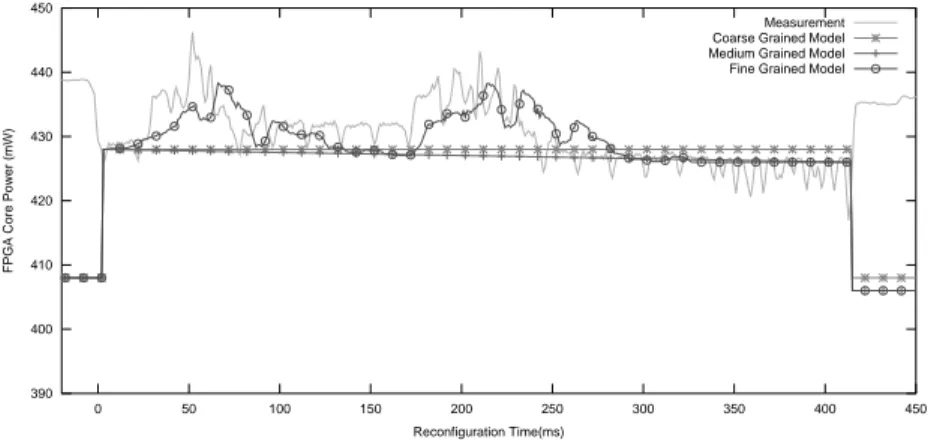
390 400 410 420 430 440 450 0 50 100 150 200 250 300 350 400 450
FPGA Core Power (mW)
Reconfiguration Time(ms)
Measurement Coarse Grained Model Medium Grained Model Fine Grained Model
Figure 9: DPR models vs. measurements for the reconfiguration of T1to T2.
by considering the idle power of previous and next tasks on the given PRR. Finally, the fine grained model provides the best estimation results with less than 6% of error in all cases, by including power surges and power steps to the model. We can thus observe in figures 9, 10, 11 and 12 a close match between the power estimated by the fine grained model (“o” round marked line) and the real measured power (straight line).
Table 2: Average standard error and root mean square error of energy estima-tions for the coarse grained (CG), medium grained (MG) and fine grained (FG) models compared to real measures (M)
Config M (mJ ) CG error (mJ ) MG err. (mJ ) FG err. (mJ ) T2 to T1 9.12 -1.3 (-13.7%) -0.84 (-9.2%) 0.5 (5.5%) T1 to T2 9.58 -0.89 (-9.2%) -1.3 (-13.5%) -0.22 (-2.3%) T1 to Tblank 7.97 6.2 (77%) 0.59 (7.4%) -0.13 (-1.7%) Tblank to T2 10.41 -7.1 (-67.9%) -2.1 (-19.7%) 0.5 (5%) Average 9.27 -0.77 (-8.3%) -0.9 (-9.8%) -0.16 (-1.8%) RMSE 4.77 (51.5%) 1.34 (14.5%) 0.38 (4.0%)
5.3
Accuracy of power profiles
In addition to the accuracy of energy estimations presented above, the ability of power profiles to predict a correct behavior is also an important quality criterion for the models. The variations of power models from actual power measurements can be indicated by computing the differences of the models with reality on each point of the profiles and taking an average. These variation values are presented in table 3 for the three models and all reconfiguration scenarios.
As expected, the results show that the coarse grained model has an impor-tant deviation of 6.5mW , which is 17.6% of the average reconfiguration power.
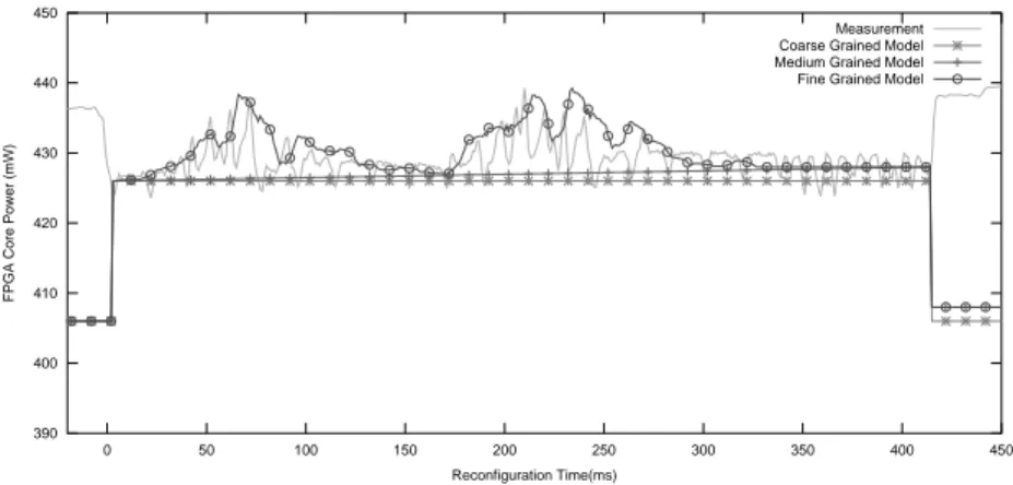
390 400 410 420 430 440 450 0 50 100 150 200 250 300 350 400 450
FPGA Core Power (mW)
Reconfiguration Time(ms)
Measurement Coarse Grained Model Medium Grained Model Fine Grained Model
Figure 10: DPR models vs. measurements for the reconfiguration of T2to T1.
390 400 410 420 430 440 450 0 50 100 150 200 250 300 350 400 450
FPGA Core Power (mW)
Reconfiguration Time(ms)
Measurement Coarse Grained Model Medium Grained Model Fine Grained Model
Figure 11: DPR models vs. measurements for the reconfiguration of T1 to
390 400 410 420 430 440 450 0 50 100 150 200 250 300 350 400 450
FPGA Core Power (mW)
Reconfiguration Time(ms)
Measurement Coarse Grained Model Medium Grained Model Fine Grained Model
Figure 12: DPR models vs. measurements for the reconfiguration of Tblank to
T2.
This error comes from not considering power surges and power steps. The medium grained model reduces the average deviation to 4.05mW (10.5%) by taking into account roughly the power steps. Finally, the fine grained model is slightly better with an average deviation of 3.75mW which is 9.6% of the average power of the reconfiguration. It might be noted here that there is an over-estimation of power surges in the computation of the Hamming distance in this case. This is caused by the dissymetry of power levels resulting from the configuration involving Tblank that can be clearly seen in figures 11 and 12.
Moreover, finer variations of power are not estimated and contribute to increase the error. However, most peak values are present and the general power trend is globally well estimated.
Table 3: Power profiles deviation for coarse grained (CG), medium grained (MG) and fine grained (FG) models, compared to measurements.
Config CG (mW ) MG (mW ) FG (mW ) T2 to T1 2.7 (5.8%) 2.7 (5.8%) 3.2 (6.9%) T1 to T2 4.9 (10.2%) 4.6 (9.5%) 3.8 (7.9%) T1 to Tblank 10 (31.8%) 5 (16%) 4.3 (13.5%) Tblank to T2 8.2 (22.4%) 3.9 (10.7%) 3.7 (10%) Average 6.5 (17.6%) 4.05 (10.5%) 3.75 (9.6%)
5.4
Relevance of DPR Models
The three models proposed for DPR are useful to adjust the estimation accuracy to the level of analysis and detail needed. In all cases, the fine grained model is preferable in terms of precision, but it is not always the best choice in pratice due to its high elaboration complexity (Hamming distance, step function and calibration parameters). In addition, the accuracy of the fine grained model is
not necessary in many cases. Especially, fine power details become secondary when the reconfiguration overhead is optimized and low compared to execution times and power of hardware tasks (which is also a requirement for actual DPR benefits). Therefore the choice of a model is driven by i) the availability of a fine grained model for a device or technology, and ii) a tradeoff between accuracy and elaboration complexity. In the absence of a fine grained model, coarse grained and middle grained models are easier to use and relevant enough to provide fair energy estimations and power profiles in a large number of cases. Next section will illustrate the practical consideration of two of these models for a realistic application example.
It is important to stress that the performance of a reconfiguration controller has also a very large impact on the relevance of DPR in a real design. In the pro-posed experimental setup of section 2.3 based on the Xilinx Reference Design, reconfiguration performance is dependent on the use of Xilinx xps_hw_icap, MicroBlaze and CompactFlash. Higher reconfiguration performance can be
reached using an optimized framework such as [Duhem, F. and Muller, F. and Lorenzini, P.(2011)]
and [Bonamy et al.(2012)Bonamy, Pham, Pillement, and Chillet]. In [Bonamy et al.(2012)Bonamy, Pham, Pillement, and Chillet] for example, reconfiguration is significantly faster but power variations are very
difficult to detect in this case because of the low level of currents involved and bandwidth limits of current probes. Measurement is the main reason why a standard Xilinx setup is used in this study. However, we have also developed optimized DPR controller IPs under closely related works and we have a precise knowledge of the mechanisms and techniques used. The steps involved in an optimized DPR process are essentially the same, therefore the same power mod-els apply. The use of an optimized controller is thus expected to affect mainly the parameters of equations and depends on the DPR model concerned. For the coarse grained model, power of the controller (Pcontrol) is the only
param-eter impacted in equation (1), performance (Tword) has also to be modified for
the medium grained model in equation (2). When considering the fine grained model of equation (3), Pcontrol is affected. In addition, faster reconfiguration
could also decrease peaks of supply current due to the capacitance effect of power rails. This can in turn impact the Hamming distance and require an ad-justment of the sliding window used for computation, to correct the amplitude of power peaks. Considering this, a relative deviation can occur for optimized controller models but in this case, this would mainly relate to the fine grained model.
6
Application Study
6.1
Overview
6.1.1 AADL Exploration and modeling framework
In this section, we show the usefulness of previous DPR models for the analysis of a relevant application example. The design framework used for this pur-pose is a system level approach based on the Architecture Analysis and Design
Figure 13: H.264/AVC decoder block diagram and profiling
Language (AADL [aad(2010)]) developed in the scope of the Open-PEOPLE platform project [ope(2013)]. In this context, a methodology automating the Design Space Exploration (DSE) of energy and performance tradeoffs in dy-namically reconfigurable systems has been proposed, allowing the evaluation of multiple application implementations on a heterogeneous System-on-Chip com-posed of processor(s) and dynamically reconfigurable unit(s). It starts from the description of execution resources (CPU cores, FPGA) and application tasks with their possible hardware and software instantiations. Then a greedy algo-rithm searches for all mapping solutions and computes the associated costs in terms of energy and performance. Reliable analysis of dynamic hardware im-plementations in particular requires relevant energy models of the dynamic and partial reconfiguration process. In the following, we illustrate the use of previous DPR models in this DSE and modeling framework for the realistic application example described in the following.
6.1.2 H264/AVC decoder
The application which is considered for this validation study is a H.264/AVC profile video decoder. High Level Synthesis (HLS) is used to provide values of cost performance tradeoffs for possible hardware functions, which serve as an entry point to the exploration methodology. The H.264 decoder used corre-sponds to the block diagram of figure 13 which is a version derived from the ITU-T reference code [h26(2005)] to comply with hardware design constraints and HLS. From the original C++ code, a profiling step identifies four main functionalities for acceleration that are, in order of importance, the deblocking filter (24%), the inverse context-adaptive variable-length coding (Inv. CAVLC 21%), the inverse quantization (Inv. Quant. 19%) and the inverse integer trans-form (Inv. Transf. 12%). To achieve better results, we have merged the inverse
Table 4: H264 task parameters
SWex HWex
HWseq HWpar
T ask Tex(ms) Tex(ms) Slices Tex(ms) Slices
Exp-Golomb 5 – – – – MB Header 4.92 – – – – Inv CAVLC 22.06 14.90 3118 – – Inv QTr 10.19 4.92 1056 3.93 1385 Inv Pred 10.77 – – – – DB Filter 34.98 3.14 686 3.11 1869
quantization and integer transform into a single block (Inv. QTr.). It might be noted here that CAVLC was not added to this block because the HLS tool (Catapult C Synthesis 2009a Release) could not handle the complexity of the resulting C code. Therefore, this results in three potential hardware functions representing 76% of the total processing time.
The deblocking filter, inverse CAVLC, and inverse quantization and trans-form block are the three functionalities of the decoder that can be either imple-mented in software or in dedicated hardware. For hardware implementations, an exploration of loop level parallelism was carried out with the HLS tool in or-der to target varying performance and resource requirements. We have selected from the results the fastest and the slowest solutions for each accelerator, except for CAVLC where too little parallelism could be exploited by the HLS tool. Ta-ble 4 shows the corresponding hardware and software task parameters that will be the inputs for the exploration example. In this table, hardware execution parameters (section HWex) are measured on a Virtex-6 LX240T FPGA (Xilinx
ML605 development board). Software tasks (section SWex) are described over
a 600MHz ARM CortexA8 processor (Texas Instruments BeagleBoard) rather than MicroBlaze in order to provide results and discussions that are more rele-vant of video processing constraints (25 fps).
6.2
Exploration Results
With the previously described exploration framework, we analyze different exe-cution possibilities of the H264 decoder envisaging a heterogeneous computing platform possibly composed of ARM CortexA8 cores and a Virtex-6 FPGA (sup-porting DPR). The exploration algorithm analyzes the power and time required for running each task using a CPU or a hardware resource (PRR). Reconfigu-ration costs are considered based on the estimation models presented in section 4. Exploration results highlights one solution corresponding to the lowest en-ergy consumption and execution time for the entire application. We chose to setup the reconfigurable resource in two PRRs of different sizes derived from the area of available hardware tasks described in table 4. The size of P RR1 and P RR2 are respectively 1200 and 3200 slices in such a way that all hardware
tasks can fit in the largest PRR (P RR2). The smallest PRR (P RR1) is suit-able only for hardware sequential implementations (HWseq) of Inv. QTr. and
DB Filter. As the reconfiguration speed of the xps_hw_icap can not exceed 15M B/s, which is too slow to meet video processing constraints, we set a faster reconfiguration throughput of 40M B/s. In these conditions, the correspond-ing exploration results are reported considercorrespond-ing the Coarse Grained and Fine Grained DPR models.
6.2.1 Coarse Grained DPR Model
Exploration results using the coarse grained model for the first execution of a hyper-period of the H264 decoder highlighted a best energy and performance DPR solution whose details are represented in figure 14. Top of this figure is the mapping of hardware and software tasks respectively on PRRs and CPUs against time. For this solution, three tasks are executed on a unique CPU (in blue) and three tasks are executed using the two PRRs (in green). We can no-tice the presence of dynamic and partial reconfiguration phases (in red) prior to each hardware task execution. As expected, reconfiguration time overheads are important (13ms for P RR2, 5ms for P RR1) but hardware DPR still outper-forms software execution by 37%. On the corresponding estimated power profile (bottom of figure 14), we can see the processor power consumption when it goes from running to idle state when Inv. Pred. task is finished (21ms). Power con-sumption of the reconfigurations, based on the coarse grained model (constant power), are represented before hardware execution (10 − 23ms, 37 − 42ms and 47 − 52ms).
6.2.2 Fine Grained DPR Model
The best energy and performance DPR solution provided by the exploration results, using now the fine grained model, is reported in figure 15. Changing the DPR model does not change the mapping of tasks which is exactly the same as described previously in figure 14. Both overall power profiles of figure 14 and 15 are very similar except in some details resulting from the sophistication of the finer grained model, putting into light additional variations impacting the power profiles. Power surges, estimated with the Hamming distance, are apparent in the global SoC power consumption. Power steps are also present e.g. at 12ms and 19ms when configuring CAVLC and at 38ms and 40ms for the configuration of Inv. QTr. These power steps are not visible for DB Filter since idle power of Inv. QTr. and DB Filter are quite similar (33.4mW and 34.2mW ).
The overall energy, execution time and maximum power estimated with both models are reported in table 5 for further discussion in the following.
6.2.3 Result Analysis
Table 5 summarizes key features of the best hardware DPR solution highlighted by exploration, for both coarse grained and fine grained estimation results. It
0 10 20 30 40 50 60 CPU1 PRR1 PRR2 Exec Time (ms) Resources ExGolomb MBHeader DPR CAVLC DPR Inv.QTr. Inv.Pred DPR DBFilter 0 10 20 30 40 50 60 0 200 400 600 800 1000 Exec Time (ms) Power (mW)
Figure 14: Task mapping, scheduling and power profile estimation using the coarse grained model.
0 10 20 30 40 50 60 CPU1 PRR1 PRR2 Exec Time (ms) Resources ExGolomb MBHeader DPR CAVLC DPR Inv.QTr. Inv.Pred DPR DBFilter 0 10 20 30 40 50 60 0 200 400 600 800 1000 Exec Time (ms) Power (mW)
Figure 15: Task mapping, scheduling and power profile estimation using the fine grained model.
Table 5: Characteristics of exploration results
Energy (mJ ) Time (ms) Max Power (mW ) Coarse Grain 31.91 54.99 748.48
Fine Grain 32.53 (1.9%) 54.99 816.5 (+9.1%) Full software 39.12 87.92 445 HW (no DPR) 25.1 31.11 953
also compares these values against full software execution (one CPU, no ac-celerator) and static hardware implementation (no DPR, all IPs are statically instantiated on the FPGA). First, the difference in energy estimations is only 0.62mJ (2%) between the fine grained and the coarse grained models. The re-duced deviation comes from the efficient modeling of power steps and power surges in the reconfiguration process. Secondly, the estimated execution time is the same for both models, which shows that small energy differences did not affect mapping choices during exploration. Finally, the maximum peak power estimated by the fine grained model is 68mW (9%) higher than the peak power estimated by the CG model. As mentioned in section 5.4, the fine grained model illustrates its ability to consider more advanced level of characteristics, global peak power in this case. In this example, the maximum SoC power consumption is visibly impacted by DPR, this can have to be considered in the development of power sensitive applications. On the flip side, the coarse grained model pro-vides simple but accurate enough model (2% energy difference) to achieve early system level estimation and exploration.
In this case study, DPR hardware / software execution of the application pro-vides noticeable acceleration and energy reduction compared to a full processor solution (based on single core CortexA8). Decoding rate is 18 frames per second (fps) while single processor execution reaches 11 fps, which is 64% faster. The energy gain is 17% for DPR against mono processor execution. However, com-pared to a static implementation of all accelerators (no DPR), the lowest energy DPR solution consumes more, 32.53mJ versus 25.10mJ . The corresponding ex-ecution times are 31ms for the static solution and 55ms for the DPR solution. It should be noted here that 24ms of this execution time (43%) is devoted to the reconfiguration overhead. Using a more efficient controller would greatly reduce this and the energy cost as well. For example, an optimized reconfiguration controller such as [Bonamy et al.(2012)Bonamy, Pham, Pillement, and Chillet] has a reconfiguration speed of 400MB/s for 384nJ/KB, compared to 96KB/s for 213uJ/KB in a Xilinx ICAP based setup. Introducing these parameters in the coarse grained model for exploration reduces the total part of reconfigura-tion time from 43% to 9% of the total execureconfigura-tion time. This also results in a lower power/energy overhead and reduces the overall energy of the best energy solution to 19.45mJ , which is then 22.5% better than a static solution.
6.3
Further analysis of estimation accuracy
To complete the analysis of estimation accuracy (section 5), six additional re-configuration scenarios using H.264 hardware tasks with a PRR of 1440 slices have been considered in table 6 and table 7: Inv QT rpar to Tblank, Tblank to
Inv QT rpar, Inv QT rparto Inv QT rseq, Inv QT rseqto DB F ilter, DB F ilter
to Inv QT rpar, Inv QT rpar to T1. When compared to the measures, energy
Table 6: Average standard error and root mean square error of energy estima-tions for the coarse grained (CG), medium grained (MG) and fine grained (FG) models compared to real measures (M)
Config M (mJ ) CG error (mJ ) MG err. (mJ ) FG err. (mJ ) Inv QT rpar to Tblank 7.4 24 (324%) 6.4 (86.8%) 6 (82%)
Tblank to Inv QT rpar 16 -12.9 (-80.6%) 2.2 (-13.7%) 10 (67%)
Inv QT rpar to Inv QT rseq 13.5 11.8 (87.5%) 0.4 (2.8%) 2.7 (19.6%)
Inv QT rseqto DB F ilter 19.2 -12.6 (-65.8%) -5.4 (-28%) 2.9 (15%)
DB F ilter to Inv QT rpar 29.1 -22.9 (-78.6%) -15.2 (-52.4%) -2.1 (-7.2%)
Inv QT rpar to T1 21.9 -1.4 (-6.6%) -8 (-36.7%) -1.7 (-7.6%)
RMSE 12.9 (89%) 6.1 (43%) 4 (27%)
estimations show larger deviations: 27% for FG, 43% for MG and 89% for CG in average. Power profiles follow the same trend: 34% for FG, 31% for MG and 44% for CG (average). Closer analysis shows that the size of tasks increases disparities of the models (e.g. Inv QT rpar with 1385 slices representing 96% of
the PRR’s resources). This means that the Hamming distance and power step modeling functions (section 4) have to be refined for PRRs and tasks of very important complexities. Additional modeling and analysis would be required to further increase the precision of DPR estimates which depends on detailed low level DPR knowledge (bitstream, PRR structure) that are protected information not easy to investigate.
However, the estimation models are intended to be used at system level ex-ploration where the current accuracy is sufficient. We chose not to develop finer DPR modeling as it is not essential for our goals and would additionally lead to technology dependent models. In previous exploration example, the improve-ment of FG over CG is due to a better matching with real power peaks (which grew by 9% using FG), and results in more accurate energy estimations. How-ever, the benefits of DPR FG modeling regarding the full application level is relatively limited (1.9% better energy accuracy over CG for the H.264 decoder example). DPR overheads in this example represent up to 43% of the total ex-ecution time due to the use of an unoptimized DPR controller for measurement reasons. In a practical implementation, reconfiguration time would be reduced to a smaller fraction of the global application execution time, limiting even fur-ther the impact of model deviations to a level that can be considered negligible (e.g. significantly below 1.9% for the H.264 application example).
Table 7: Power profiles deviation for coarse grained (CG), medium grained (MG) and fine grained (FG) models, compared to measurements.
Config CG (mW ) MG (mW ) FG (mW ) Inv QT rpar to Tblank 15.2 (142%) 5 (47%) 10.1 (94%)
Tblank to Inv QT rpar 13.7 (59%) 6.3 (27%) 10.1(44%)
Inv QT rpar to Inv QT rseq 17.7 (91%) 10.5 (54%) 12 (62%)
Inv QT rseq to DB F ilter 6.6 (24%) 6.5 (23%) 6.8 (23%)
DB F ilter to Inv QT rpar 12.7 (30%) 16.5 (39%) 15 (35%)
Inv QT rpar to T1 16.9 (53%) 13.7 (43%) 13.5 (43%)
Average 10.8 (44%) 7.5 (31%) 8.3 (34%)
7
Conclusion and Perspectives
Based on a reference procedure of dynamic and partial reconfiguration for Xilinx FPGAs, this paper has thoroughly investigated the measurements and model-ing of power and energy durmodel-ing run-time partial reconfiguration. Results have shown that power consumption was not as straightforward as expected. Compo-nents other than the reconfiguration controller have been identified, like the ef-fect of previous configuration and the resources of reconfigurable regions. Three analytic models have been proposed in order to help analyzing the power contri-bution of dynamic reconfiguration at different levels of detail. The applicability and usefulness of these models have been illustrated on a representative example of design space exploration for a H264/AVC decoder. In this application study, the ability of models to determine if exploiting DPR in a SoC actually leads to an overall energy saving or to a loss has also been shown.
The perspectives from this work1 are to continue developing the applica-bility, especially for more generic model calibration and interaction between models and tools. Another issue in this context is also to investigate online multiprocessor scheduling policies that would be able to support efficient execu-tion of dynamic hardware and software tasks. The expected results from these efforts are a complete system level approach for the design space exploration of reconfigurable heterogeneous multicore System-on-Chips with power issues.
Vitae
Robin Bonamy received his M.E. degree in Electronics and Embed-ded Systems from University of Rennes, France in 2009 and his Ph.D. degree in signal processing at IRISA, France in 2013. He is currently occupying a postdoc position. His research interests are power and energy models and design space exploration especially for energy con-sumption reduction in micro-controllers, FPGAs and reconfigurable devices.
1This work was carried out under the Open-PEOPLE project, a platform project
funded within the framework of the Embedded Systems and Large Infrastructures program (ARPEGE) from ANR, the french National Agency for Research.
Sebastien Bilavarn received the B.S. and M.S. degrees from the University of Rennes in 1998, and the Ph.D. degree in electrical en-gineering from the University of South Brittany in 2002 (at formerly LESTER, now Lab-STICC). Then he joined the Signal Processing Laboratories at the Swiss Federal Institute of Technology (EPFL) for a three year post-doc fellowship to conduct research with the Sys-tem Technology Labs at Intel Corp., Santa Clara. Since 2006 he is an Associate Professor at Polytech’Nice-Sophia school of engineering, and LEAT Laboratory, University of Nice-Sophia Antipolis - CNRS. His research interests are in design, exploration and optimization from early specifications with investigations in heterogeneous, recon-figurable and multiprocessor architectures, on a number of french, european and international collaborative research projects.
Daniel CHILLET is member of the Cairn Team, which is an Inria Team located between Lannion and Rennes in France. Daniel CHIL-LET received the Engineering degree and the M.S. degree in elec-tronics and signal processing engineering from University of Rennes 1, respectively, in 1992 and in 1994, the Ph.D. degree in signal pro-cessing and telecommunications from the University of Rennes 1 in 1997, and the habilitation to supervise PhD in 2010. He is currently an Associate Professor of electrical engineering at the Enssat, engi-neering school of University of Rennes 1. Since 2010, he is the Head of the Electronics Engineering department of Enssat. His research in-terests include memory hierarchy, reconfigurable resources, real-time systems, and middleware. All these topics are studied in the context of MPSoC design for embedded systems. Low power design based on reconfigurable systems is one important topic and spatio-temporal scheduling, memory organization and operating system services have been previously addressed on several projects.
Olivier Sentieys joined University of Rennes (ENSSAT) and IRISA Laboratory, France, as a full Professor of Electronics Engineering, in 2002. He is leading the CAIRN Research Team common to INRIA Institute (national research institute in computer science) and IRISA Lab. (research institute in computer science and random systems). Since September 2012 he is on secondment at INRIA as a Senior Re-search Director. His reRe-search activities are in the two complementary fields of embedded systems and signal processing. Roughly, he works firstly on the definition of new system-on-chip architectures, espe-cially the paradigm of reconfigurable systems, and their associated CAD tools, and secondly on some aspects of signal processing like finite arithmetic effects and cooperation in mobile systems. He is the author or coauthor of more than 150 journal publications or peer-reviewed conference papers and holds 5 patents. Olivier Sentieys is the head of the Architecture department of IRISA.
References
[Lemoine and Merceron(1995)] E. Lemoine, D. Merceron, Run time reconfiguration of FPGA for scanning genomic databases, in: FPGAs for Custom Computing Machines, 1995. Proceedings. IEEE Symposium on, 1995.
[Tadigotla et al.(2006)Tadigotla, Sliger, and Commuri] V. Tadigotla, L. Sliger, S. Commuri, FPGA implementation of dynamic run-time behavior reconfig-uration in robots, in: Computer Aided Control System Design, 2006 IEEE International Conference on Control Applications, 2006 IEEE International Symposium on Intelligent Control, 2006 IEEE, 2006.
[Eldredge and Hutchings(1996)] J. G. Eldredge, B. L. Hutchings, Run-Time Recon-figuration: A Method for Enhancing the Functional Density of SRAM-based FP-GAs, The Journal of VLSI Signal Processing 12 (1996) 67–86.
[Zhang et al.(2008)Zhang, Rabah, and Weber] X. Zhang, H. Rabah, S. Weber, Dy-namic slowdown and partial reconfiguration to optimize energy in fpga based auto-adaptive sopc, in: Electronic Design, Test and Applications, 2008. DELTA 2008. 4th IEEE International Symposium on, 2008.
[Sterpone et al.(2011)Sterpone, Carro, Matos, Wong, and Fakhar] L. Sterpone, L. Carro, D. Matos, S. Wong, F. Fakhar, A new reconfigurable clock-gating technique for low power SRAM-based FPGAs, in: Design, Automation & Test in Europe Conference & Exhibition (DATE), 2011, 2011.
[Claus et al.(2008)Claus, Zhang, Stechele, Braun, Hubner, and Becker] C. Claus, B. Zhang, W. Stechele, L. Braun, M. Hubner, J. Becker, A multi-platform controller allowing for maximum dynamic partial reconfiguration throughput, in: Field Programmable Logic and Applications, 2008. FPL 2008. International Conference on, 2008.
[Rullmann and Merker(2008)] M. Rullmann, R. Merker, A cost model for partial dy-namic reconfiguration, in: Embedded Computer Systems: Architectures, Model-ing, and Simulation, 2008. SAMOS 2008. International Conference on, 2008. [Duhem et al.(2012)Duhem, Muller, and Lorenzini] F. Duhem, F. Muller, P.
Loren-zini, Reconfiguration time overhead on field programmable gate arrays: reduction and cost model, Computers & Digital Techniques, IET 6 (2012) 105–113. [Becker et al.(2003)Becker, Huebner, and Ullmann] J. Becker, M. Huebner, M.
Ull-mann, Power estimation and power measurement of Xilinx Virtex FPGAs: trade-offs and limitations, in: Integrated Circuits and Systems Design, 2003. SBCCI 2003. Proceedings. 16th Symposium on, 2003.
[Lorenz et al.(2004)Lorenz, Mengibar, Valderas, and Entrena] M. Lorenz, L. Men-gibar, M. Valderas, L. Entrena, Power consumption reduction through dynamic reconfiguration, in: Field Programmable Logic and Application, Springer Berlin / Heidelberg, 2004.
[Bonamy et al.(2012)Bonamy, Pham, Pillement, and Chillet] R. Bonamy, H.-M. Pham, S. Pillement, D. Chillet, UPaRC - Ultra Fast Power aware Reconfig-uration Controller, in: Design, Automation & Test in Europe Conference & Exhibition (DATE), 2012.
[ope(2013)] Open-PEOPLE - Open-Power and Energy Optimization PLatform and Estimator, http://www.open-people.fr/, 2013.
[ML5(2013)] Virtex-5 LXT ML550 Networking Interface & Power Measure-ment Platform, http://www.xilinx.com/products/boards-and-kits/ HW-V5-ML550-UNI-G.htm, 2013.
[Xilinx(2011)] Xilinx, UG744 - PlanAhead Software Tutorial: Partial Reconfiguration of a Processor Peripheral, 2011.
[Bonamy et al.(2011)Bonamy, Chillet, Sentieys, and Bilavarn] R. Bonamy, D. Chillet, O. Sentieys, S. Bilavarn, Parallelism Level Impact on Energy Consumption in Reconfigurable Devices, ACM SIGARCH Computer Architecture News 39 (2011) 104–105.
[Liu et al.(2010)Liu, Pittman, and Forin] S. Liu, R. N. Pittman, A. Forin, En-ergy reduction with run-time partial reconfiguration, in: Proceedings of the ACM/SIGDA International Symposium on Field Programmable Gate Arrays, 2010.
[Xilinx(2010)] Xilinx, UG191 - Virtex-5 FPGA Configuration User Guide, 2010. [Duhem, F. and Muller, F. and Lorenzini, P.(2011)] Duhem, F. and Muller, F. and
Lorenzini, P., FaRM: Fast Reconfiguration Manager for Reducing Reconfiguration Time Overhead on FPGA, in: Reconfigurable Computing: Architectures, Tools and Applications, Springer Berlin / Heidelberg, 2011.
[aad(2010)] Architecture Analysis & Design Language (AADL), version 2, http:// standards.sae.org/as5506a/, 2010.
[h26(2005)] ISO/IEC 14496-10, Advanced Video Coding for Generic Audiovisual Ser-vices, ITU-T Recommendation H.264, Version 4, 2005.