HAL Id: tel-01818034
https://tel.archives-ouvertes.fr/tel-01818034
Submitted on 18 Jun 2018
HAL is a multi-disciplinary open access
archive for the deposit and dissemination of sci-entific research documents, whether they are pub-lished or not. The documents may come from teaching and research institutions in France or abroad, or from public or private research centers.
L’archive ouverte pluridisciplinaire HAL, est destinée au dépôt et à la diffusion de documents scientifiques de niveau recherche, publiés ou non, émanant des établissements d’enseignement et de recherche français ou étrangers, des laboratoires publics ou privés.
Ecological niche modelling and its application to
environmentally acquired diseases, the case of
Mycobacterium ulcerans and the Buruli ulcer
Kevin Carolan
To cite this version:
Kevin Carolan. Ecological niche modelling and its application to environmentally acquired diseases, the case of Mycobacterium ulcerans and the Buruli ulcer. Infectious diseases. Université Montpellier II - Sciences et Techniques du Languedoc, 2014. English. �NNT : 2014MON20178�. �tel-01818034�
!
"
#
! ! !
$
% &
'
( )
$*
+
!
, -
!
.
&/ ,
0 & '1 2 3 0 ,
/2,4 '' 0
4
!
!
!. !
5
.
657
! " # # $$ % &' ( " ) * + + , -$ * , -& +. * ! + + , ! + + ) / & +. 0 " 0 + + , )
1 2+ + ) + 3 4 2+ 5 6 ) + ) + 3 7 8 + ) + 7 9 + 0 + ) + 0 0 : ; + / ) + ) + : < ! ) + ) 14 # ) 6 = + + + ) + 14 2 6 + ) 1> $ ) 1> 1? 0 4@ 0 6+ + + 44 6 + + 4; 4> 7@ ' 6 71 A0 74 $ 74 # # + 7< ;4 * ;; ;B ! ! " ;? ' 6 ;C A + >@ 5) >@ # + ) >7 BC * <7 <> <B # $ % & ! ' ( ! ) " ?@ ' 6 ?1 A0 ?7 5) ?; # # + ?B C4 * C< 1@@
* + " 1@4 $ 1@7 ) + = 1@7 8+ ) + 1@; 8+ + 0 6 1@C / + 114 11> 11B , - &" 11< ' 6 11? # + 6 ) ) )
" D & E + &0 0 + & /
+ )
. / ' ) 1 > ' ) 4 B ' ) 7 ? ' ) ; C ' ) > 1@ ' ) B 1; ' ) < 1; ' ) ? 1> ' ) C 1< ' ) 1@ 1C ' ) 11 41 ' ) 14 44 ' ) 17 47 ' ) 1; 71 ' ) 1> 7; ' ) 1B 7> ' ) 1< 7B ' ) 1? 7? ' ) 1C ;@ ' ) 4@ ;4 ' ) 41 ;7 ' ) 44 >; ' ) 47 >C ' ) 4; B; ' ) 4> B< ' ) 4B B? ' ) 4< <@ ' ) 4? <4 ' ) 4C ?4 ' ) 7@ ?B ' ) 71 ?C ' ) 74 C1 ' ) 77 C4 ' ) 7; C> ' ) 7> CB ' ) 7B 117
. 8 0 1 >> 8 0 4 >B 8 0 7 B1 8 0 ; B4 8 0 > B; 8 0 B B> 8 0 < <1 8 0 ? ?? 8 0 C C7 8 0 1@ C> . $0 / 1 >< / 4 ?< 77 114 2 11? ) B + 7B ' ) 1@ 8 0 4 /
- 1 " + 5 ) * ! % &' ( " ) : 8+ + + 0 0 + + 0 0 : * % &' ( + 0 6 + 0 + 5 : $ 6 5 + 5 + A 8 9 + ) # 0 )+ ) + 6+ + 5 ) +: + 5 5 ) + 5 F G + + : $ + 7 $ + 0 + $ + + * # 8 + 5 ) + $ * #8* + $ ! 0 A : 8+ & + A " + * + " 0 " & % ! # A # ) # H 0 ) " I 8 ! # + ! " A ' + " ) + : 8+ 5 + +*- $ * # # + A ) = # + 8 + = + J + ' + A # " ) + K 0 ) : 8 ! L + 6 $ 5 6 6+ 5 + + : A # * = 0 ) + :
!"# $ %% & ' ( %%! % %) & * + , ) -. . ) + -( . ! # / 0 1 ) 1 0 ! #) 0 ! ! 1 2 0 + ) !"#)
3 * ) 4 5 %%3) %%6 7 % 3 0 % % & %%!) 4 % 3) 7 * !"#) + + 48 * 9 * : !"#) 48 ) . -9 ; ( * 8 & ' ( %%!) + 8 7 :; :, 7;, ) & ' ( %%! : : ) )
< 7;, 2 7;, * 2 ) ) + ( : + 3 0 %%=) . > ( %%")
" + ) ) ) ) 48 * . 1 8 . 8 ? @ A 1 @ A 1 ? ? ; 1 ; - + 7 ' 2 ) 1 < & ? ? ? 1? 0 5 > 8 48 0 10 20 30 40 50 0 2 4 6 8 1 0 Oxygen concentration P o p u la ti o n s iz e 0 10 20 30 40 50 0 2 4 6 8 1 0 pH P o p u la ti o n s iz e 0 10 20 30 40 50 0 2 4 6 8 1 0 UV light P o p u la ti o n s iz e
= + 8 + ) 2 : ? ? ) B ) ) 7 B B 48 9 , : B 3 ) 5 : ; . @ A %% )
Projection into different environmental contexts G P O L
Real space
0 5 10 20Km Region 1 Region 2 Region 3 0 5 10 20Km 0 5 10 20KmVenn representation
# ! " # " * & ; C2 %%< ; %%# & ' ( %%!) - . -- 1 $ + 3) ( + <) ; D %%<) $ ; ' . - -5 : - 5 E % % 1 ) 9 F & + 51B) G'; 9 G'; + " 2 - 51B + : - 1 1
6 + 3 & ) ) 1 ) & 4 Species distribution data Environmental gradient data
Inference of suitability Distribution of suitable habitat 0 10 20 30 40 50 0 2 4 6 8 10 Intensity of UV light
Population size of a hypoth
etical species 0 10 20 30 40 50 0 2 4 6 8 10 O xygen concentration Popula tion size of a h ypothetical species 0 10 20 30 40 50 0 2 4 6 8 10 pH
Population size of a hypothetical s
! + < & 7 48 * 1 -+ ( Oxygen pH UV light & 4 Physiology a priori understanding of suitability Distribution of environmental of conditions Distribution of suitable habitat
% + " + 3 * ( ) . G 1 ) G . Observed distribution 0 10 20 30 40 50 0 2 4 6 8 10
Int ensity of UV light
Population size of a hyp
oth etical species 0 10 20 30 40 50 0 2 4 6 8 10 Oxygen concentration Population size of a h ypothetical species 0 10 20 30 40 50 0 2 4 6 8 10 pH P
opulation size of a hypothetical s
pecies
Where the species is
Variation in detectability
Environmental gradient data
Inference of suitability Distribution of suitable habitat
0 %% ) H ) I ) HJ K K > ( + 0 !!") ( > 7 ( 0 $ 0>,) 0 %% ) - 5 0 * ) ) 0 $ 0;,) ( 0>, L %%!) 0;, 0>, ( : 0>,A 0;,A , %%6) 0>, 1 , %%6) ; ( ) : , ) ) 5 D (E> ) 5 %%6) ( = %%=) . %%=) ,
$ %% ) 0 : 5 7 1 %% ) ) ' 5 3 < + : M " " . * $ + " 9 ) F $ % & " " ; & ( !!#) ; + =) +
3 48 5 !!6 & %%# , % % 0 % <) * & 1 % < + #) 1 1 %%") ) + =) ; -) . 4 . 1 + 0 D 7 ;
< + = ; ; -1 N D 1 > 0 0 * % %) + # ; ( ; : B 1 % <)
" % ' 7 * 1 ; 1 ; / + 0 : + & ; ) ; + 6 * ; " %%% % %%% / %%") + 6 0 7 %%6 % % % % < 2 * 1 ; + 0 ; / - B *
= 1 7 . ( ' + 0 , % <) . ;( 1 9 ' > % <) > 7 0 :8 ( % <) 5 ( 4 + !) ( %%") ) 1 ;
# + ! . ( * ( 1 : ( B / %%")
6 ( ' " . 7 + ' B ; O ;'B) 2 P ! $ M Q ) *+,$-) % ;'B 1 5> %%# %< I B;:,4) 2 ( 2 ( I B;:,4 2 1 ' B & - 1'B&) . 5 , . 8 M R 0O O - R 1 S ,.8 0 1) / O- O T U.BG ; , / ;. ; , ) . B GO .BG) O O O . & .&) 1 O -O 1.B;G) G & V . O O 7 ; 0O &.7;0 ) 4 O , ; 1 5 1 I B;:,4 2 7 1 * ( 1 O -O V : S : 7. 5&H&) > U M 1 AO O $ > :1 7;) > 1 7; ; $ + 0 7 7. 5&H& 2 I B;:,4 / ;. ; , 7. 5&H& ( $ 5 G % -& %%%)
-! -( + % > %%3) 48 + % B B > %%3) N %%3 . G & ; ( - ,4,%% ) -- -& %%#) $
% 5 ( %%3) # ) 48 , 1 %%#) , ( 0 %%%) 7 1 %%#) % " ( ( 7 ( - ; , % %) ; / %%#) - 2 ( - - ) * %%6) 7 ) : * %%6) ) 5 ( -) ) 0 + 7 % 3 , . % < 0 W :5 X Y1 =Z)
+ ;) 7 ( 1 7) 7 ( N D 1 % G -51B ; G'; -5 !!! & %%% 5 %% %%< , %%< %%< D ( %%< / %%# + %%# * %%6 5 %%6 + % % , % % B % 3 1 % < , % < 0 % <) ; ; ; . ; 1 % <) ( 7 ( ( ) ; ( / %%") ( 0 ; ) , 9
;)
7)
; ) + 2 ( + 5 ; 7 ; '?+ . & ; ; $ '?+ $ $ $ '?+?$ * " ( ( -;- ( 7 , %% ) ( 7 %%6) ;-+ ' 7 + 3) ( 7 ( B A B A M B A M
Scenario 1, evolution of the bacterium Scenario 2, range expansion of the bacterium
A fr ic a A u s tr a lia B A
3 , %% ) -( ( 7 ; ( -0 * % <) ( . ; $ !! B !!#) - ; 48 ( B $ ; % <) + 3 - ) 1 + 7 A ;) 7) + ' 1) , G) + ' B ) + 0 +) + 0) + 1 ) & B , % %
< % % . " %%% % %%% ( $ -( 7 . 1 -$ 1 3 1 < 1 "
" * ; ' [. B + : ; B [ ! % <) G .M % 3# \2 %%%3 <6 ; , [& M [ " %% %%#)M : ! 7 [;- , ; 0 * ; M 4 ' G [ " % 3)M : = 7 [;- ( 7 [ " # < 6 %%6)M <# 7 & [ [ % 3)M "%<E"%# M % %36\ %=% 1 1 [5 * & , & 7 4 & : ; [ 6 % <)M ==6 1 B [* M [ $ " % <) 1 [, , M [ % # 6 %%")M 6#: != 1 [& , [ & # %< = %%#)M 3!": <%3 , [5 , 7 )M [ #% ! %%<)M "=#!:"=6 / [' A [ " ! %%=)M !: " / [ : [ < % %)M 33%:3< & [ : , 7 [ <! 6 %%")M 3 6 :3 6= + / [G : 51B , [ #3 " %%#)M <#33:<#<% + / [; 2 , [ < 6 % %)M #!
= 0 ; [, G . ; + ;- 1 M B :, & 1 [ 6 " % <)M 6#! 0 D [; , [ ' # =6 %%%)M 6##:663 0 5 [1 [ <=" # != % %)M 3< : 3<" 0 :8 ( [ $$ 7 : P Q ;( 1 [ ( % <) G .M % % =\2 % < %3 %%6 0 0 [ ( > [ & # 6" # !!")M !<<:!<6 0 G [B M [ " ! < %%=)M 3!!:<%! 0 ; [0 $ $ M [ " "# %% )M 6!: %% & [7 [ % < % 3)M %% < 3 G [. M ( [ 1 7 = " %% )M 3# : 36" / [5 , [ ' ) # % < !! )M %!3: %!6 $ ; [ : M : F [ " 63 # %% )M % #: %3= 0 !"#) [1 ( [ 5G+) 1 & & ] 7 )M < "E< # / 5 G [, - ( 7 ; [ " ' # ! 3 %%#)M ="3: ==% D [, M $ [ " 6" %%<)M 3 !:3 3 D ( B [ : G'; 51B: , - [ & # "3 ! %%<)M ! #:!33
# > / P& : ( 7 ;( 1 Q % <) G .M % 3# \2 %%%3 3 > + [+ ( , M ( [ % # 3# 3 %%3)M 3!%:3!# > ( / [ [ ^ % " %%")M 3: 6 , & [1 ( M [ " % !!!)M 33#:3<# , [& , M [ < # % %)M #3 , > [;- , [ =6 ! %% )M <= 3:<= 6 , > [;-, [ #% %%<)M %!#: %3 , . , [; , -* ; M 7 [ " % <)M : 3 , B [ [ " 6 %%6)M 3##:3!% , B [ 7 M [ < % %)M ! , ; [+ G , G'; & & ; [ 6 % <)M ==% , ; [1 : [ " ( ' # 3 6 % <)M "= 5 / 1 [ , 7;1 1 [ & # 3= !!6)M 3< %:3< 5 ( / [1 - 7 * * [ 3" %%3)M 3 :<% 5 ; [5 , [ ' << %% )M #: 3 5 ; [4 :' , 5 7 . . & 1 [ % * # < %%3)M = : ="
6 5 + [. [ 3"3 ! "# !!!)M !6= 5 + [, [ + # , , -' .## # " / 0 % %% )M " 5 + [+ $ , [ 3 %%6)M #6 B 7 [. ; : M ( @ A , [ " + 6 < % 3)M %<"%%! B 7 1 [G , ( [ =3 % !!#)M < 3":< 36 & 5 ; 2 , [; [ & # * 3 % %%<)M """: "=6 & _ / ' ( , [' M [ # # %= & %%!)M !=<<: !="% & + [ ; 1 M [ * % ! %%!)M # & [. , & ; - :51B [ == 6 %%%)M 3 %=:3 3 & [B , 7 [ 1 # %%#)M ! : %% G D 5 & M 8 3% 5 4 5 !!# D [1 $ , : ( ; I ) [ % "< 3 %%<)M 3%!:3 # ; [4 ; G M 1 ) & + [ ' & # 1 # %%6)M ! * [; : , 7 ) 7 * ; [ " " %%6)M =!:#! * [G , 7 : - 0 [ 3 %%6)M %"
!
* [, + . &( ; 0 5
. , M . [ 6 < % <)M ##%
3 . / / . P FQ D 1 G > & / :+ ` 0 O * I B;:,4 7. 5&H& 2 . ( 2 $ * I B;:,4 2 ; 0 1 + <) 7 ;( 7 ( , 5 V 7 ; > :1 7; 7. 5&H& 7 4 ; , ( ( + 0 ;( 7 ( 7 + 0 ) $ $ 0 ( .BG9 ; 0 7 2 B ; 1.B;G 2 + < + ( ; , + 0 0 ) ( , 7 7 ) ; 0 ( 1 B ) 0 1,500 3,000 6,000Km
3 + ; -: $ -$ : - * , * $ & ( $ F ; ',) !"# & _ ' ( %%!) ', 5 B %%3) , %%<) ; %%! , % G $ ( % 3 % 3) 0 ', F ( F . $ $ ; 9 "%%
33 " - "%% $ " "%% ', . ', !"#) 8 7 :; :, 7;,) & _ ' ( %%!) + " * 7;, 9 -& % ) + " # + " '?+ 9 ', '?+?$0 '?+) $0) . '?+?$1 7;, 9 + =; '?+ '?+ J ' A ; 5 & ( G , %%<) . + =7 + !<3 - 2 : ( + %%6) * 7;, '?+1?$9 -'?+?$
3< + " 7 :; :, 7;,) G ; ' $ ) + '?+ P ' +Q) '?+?$ : ) '?+?$ 1 $0 P $Q $ '?+?$0
3" + = G 7;, 7;, + ) ) . ; $ '?+?$ '?+ J ' : ) . 7 ) ( '0?+?$ '?+0?$ '0 +0 ) + * ) ; 7;, . + = '?+ =7 =; -', -$ %%=) 9 + # ; ) ) '?+ $ '?+
3= + # & 7;, B 2 3 + 2 '?+?$? 2 0 ) 1 $ -',9 $ '?+ 7;, 7;, 8 G * %%! 7 % % ) $ ) 8) ) $ : -* ;41) , !!%) * 7;, - $ * : * :
3# 5 G W( & %%< G W( 5 & %%#) , 5 ; & %%=) : ; %%=) * ;41 , 9 8 0 ;41 ;41 $ $ $ ) 8) ) ;41 - * ;41 ;41 - ( M ) $ F - " "% "9 & $ ;41 ) $ ) F '?+) 9 " 3) F $ ) ;41 2 4 + 6 . ; " 2 *
36 + 6 2 4 : 4 D + * ' M " ) ) a %) ( * 2 %%") 4 D + ! ) + 0 %%! " a a5)\3 5 + ! ( 2 + ! ) + B 1 % 3) ;
-3! * , 5 G W( & %%<) . D (E> 5 G W( & %%<) + ) ( , 3 3 3( 5 G ( & %%# , & 3 3 3() - * " 8) % $ ) " ) , %% " %%%
<%
+ ! ;
< " # * $ ;41 ;41 $ > %%6) ;41 , ; ;41 % " % " + . : , , : : : 9 , ;41 9 ;41 ;41 %b * ;41 : ;41 ;41 ;41 ;41
< * * ;41 $ $ + %) + ) ;41 ;41 : , ;41 ;41) $ + %) $ -+ % $ 8) $ ) ;41 ;41 B ( 2 1 $ + " ;41 ;41 %% , ;41 ;41 %b , ;41 ;41 ( : , ;41 : : ;41 ;41 ;41 ;41
<3 + ) $ ) ;41 ;41 + + <) ;41 ;41 > ;41 ;41 ;41 $ ( $ ;41 ;41 ;41 5 ;41 ;41 + $ ;41 + ) ;41 + ) , ;41 ;41 : : ;41 : ( : ;41 . $ -;41 , ;41 - -$
<< 5 F + (9 ( F * ( ( * $ - ) ', $ '?+ + ") + #) $ - - 5 : : ;41 + = #) $ A 9 $ ;41 * %%3) ;41 9 -, : ( - 0 %%!) : '+; $ %% ) * - 7 %%= 8 %%!) * $ 9 + !) + ( ;41 : \ ) * %%3) ; $ '?+ ) ;41 ( 9 $ - ', . $ )
-<" B . $ * 2 , && D 5 % %) 1 - $ + : -9 9
<= * ; B %%=) ' A ! )M !: " ; G [ 2 1 [ , / 6 %%!)M 3%# 7 ' % ) " 333 ) 6 %: 6 ! G $ ( 5 % 3) . M ' # # 445 & ) 3=6 :3=66 G W( , %%#) , G 0 $ B $ ; & G , & # + 6 =) / % ) ; , ! ! 47 ) <3:"# / 0 1 %%!) G F F * H F " 83 ) ==:## / D , 5 & % %) : 4 <) 33%:3< & % 3) 7 45 <) %% < 3 $ 5 %%=) $ " 39 ") ##3:#6" 2 B %%") 8 ' ) # 3: ") !=": !#6 $ ; %% ) : M : F " 68 #) % #: %3= 7 & / %%=) & # " ;8 3) < 3:< 3 0 !"#) [1 ( [ 5G+) 1 & & ] 7 )M < "E< # > /, %%6) ;41M 1 * 47 ) <": " , B %%<) , ( ( 1 $ " 355 ) !": <
<# , / % ) ' , 7 ; : D $ ( * % 44 ) 3 , / ' [; [ * &< * & 3%% =# ! !!%)M 3% & % ) 8 M ( " 387 : & _ / ' ( , %%!) ' M # # 45= & ) !=<<: !="% 5 & / G W( , & B %%<) ; # > ?# # 63) ;1, 5 &/ ; B5 & B %%=) , " 495 3) 3 : "! 5 ; B 1B %%3) 4 :' , 5 7 . . & 1 % * 47 <) = : =" B 1 % 3) BM ; B + & 1 8 ; 4B> M\\ B: 2 \ ; [4 ; G M 1 ) & + [ . / 0 # %%6)M ! 8 & %%!) . -F ; & # * 8= !) =<": ="" 8 G * / %%!) & : : M ( F 335 <) "6!:"!< * %%3) ' : . 4= 3) %: #
<6
<! . / 2 5> & ' G P - Q D 1 ; 0 0 0 :5 ; , / > ; + 5 > 0 0 c > , B 0 $ & G > & / : + 0 O 1 ; 0 . ( + 0 ; , ; 1 + 0 & + 0 & ; ; ( ( ; 9 ; , 1 '8. & &5 B > ( 1 ' % ( & 0 c 1 5 1 ) + -; O 0 5 G R O O - &5) ; , 5 G 7 4 0 0 W :5 X + + B 7 O 1 &;7 7. G.&) . ( ( ; 1.B;G 7 2 B .BG
.&.& & - &5 O 1
"% + 6 "" , ( 1 ; * * ( ; & ; ' D ( $ H <b % 3) ( . ; + 5 !!6) , %%<;) . - $ -!"# & %%") D %%6 ; %%! ; % ) +
-" - ( * + + * ( * ( -7 * 7 $ , ( $ % %%% 3% / %%" * %%6) . 7 * %%6) $ ( / %%") ( , %% 7 %%6) ( . ( , % % ) 5 ( . %%#
-" ( & %%#) G 51B9 5 %%6) -) G'; -5 !!! & %%% 5 %% %%< , %%<; %%< D ( %%< / %%# + %%# * %%6 5 %%6 + % % B % 3 1 % < , % < ; 0 % <) A , %%<7 , %%6 , % %) -" " ( , % %) 5 ( ) ) 0 7 % 3 , . % <) * %%6 ;) ( , % %) 0 % <) 9 7 ( * % ) ( B
"3 % , % < 7) ( 9 * - ( 7 %%6 0 % <) -- 1 1 ; * + 0 $ 7 $ ; ;( 1 + 0 & ; 1 0 % <) = ;( + ) . . < -" -;- + #%b . G'; - 51B ; " G 1 ) 5 $ G';
"< ].;- ( != 51B 5 D ].;0 ') + ,4 G'; - 51B ( 7 DB) ( .& <%< - ,4 " $ ) & & 0 % <) + > 1 0 % < * 1 ;( ' B ;( ; + 0 & ; , % <) G'; . + 0 G / " ;( )
"" ;( 1 = -G 1 2 B " \ " ) 51B " 0 % <) * G & 1 > > B " b) 51B " B " b) 51B " ; '3d<= 6%= d = 33 & !3 =! = !6b 3\<3) !# 3! %b <\ %) ; '3d<# %63 d " 363 & !< =! 3=b \6!) !< "3 6 b 3\3#) ;3 '3d<= 3 = d < <<% & !% 6 "=b \3!) !% < %b %\ %) ;< '3d"6 <=< d < #!= B "" " 3b \3!) 3 # " =b \ !) ;" '<d% "" d " = % & 63 =< %b <\<%) #" 3% " =b \ !) ;= '3d<3 <63 d = <== & !% 3 # <b "\6#) 6" 6" !<b \3<) ;# '3d36 66! d " !6= B #! " % =b <\3!) #! 3 %b %\ 3) ;6 '3d36 !6% d < =!= B =< 6= ! %!b <\<<) #3 6! # =!b \ 3) ;! '3d ! ! d%= < " & 6 <% < <b <\! ) ! =# #b \3#) ; % '3d ! ! d%= < " & !3 = # "b 3\<%) 6! !% %b %\ %) ; '3d 3 # d%# 6#% B "% < ="b <\6=) "! "= 6 6 b 3\3<) ; '3d 6 #66 d%# "" B " 6# <<b \< ) == ! "b 3\ %) ; 3 '3d3 3 d"# =<3 & 6 ! b \!%) #! 3! 6 b 3\3#) ; < '3d36 %3 d"! =!" B =< ## " 36b =\3!) =3 3# %b <\ %) ; " '3d3 66 d"" 3! + !< 33 b <\3=) !# "< %b %\ ") ; = '3d3 #= d"" 6 & 6! 6" 6=b \3") !3 <% %b %\ ")
"= + 0 & ; 6 - G 1 ;( 2 B " \ " ) 51B " , % < ;) * & 1 > > B " b) 51B " b \ ) +0 % '< << #% *:" ! = 6 "6 = << b "\3<) +0 '< "% 6< *:" !" " "< 3 =b %\3 ) +0 ! '" # ##3 *:"3 %3 %6" = "% % %%b \ %) +0 '" 3# 666 *:"3 < <33 #% 63 #=b =\" ) +0 3 '" # < *:"3 % %% ! # = =#b \ ) +0 6 '" 3= 3 6 *:"3 <! ==% "= =% % %%b =\3%) +03< '< "% %=6 *:" 6 = 6" %% 3 3"b \3<) +036 '" 3 =<= *:" "! " #3 #< 3 #%b %\#3) +0< '" " # " *:"3 %" 3 = < %# 6 #%b \ 3) +0<3 '" =3 *:" "# 3 #" <# "%b \<%) +0<< '< % %" *:" %! <6 " < % %%b %\ ") +0<" '< 6 % " *:" %# 3!# = !" 6=b \#%) +0<= '" % *:" 3% !6! #< < %<b \<!) +0<# '< "" #<< *:" < ! =" %% % %%b %\ =) +0<6 '< " = = *:" = " 6 = =# % %%b %\ ) +0<! '" 3! !!= *:"3 <= #!< 3= "< % %%b %\ !) +0"3 '" 3= 3= *:"3 "% 6 =# 6= % %%b %\"#) +0# '< " =<6 *:" " <%" ! < % %%b %\ %) ## * %%6 ; , % < 7) . 1 ; , / ; & / + , / ' G + " ) H H "
"# > ;( 9 &5 " M "%63336%6 %! 3%! 8% "%6333# % %!3#< 8%) > ># 6=%"=e%"= %% %#) 9 ; + + B & & 4 3) 1 2 . ; 1 1 ' > ) ' % & B , &B ,) / %%6) !% ; & ; ; , % &B. % ) + &B , 3) + &B , + * * 7 + & ; ; , & ) 5 6 & & !"#) + . - *. 7 D ( !#!) +; & * ) )
-"6 ' # ## ## + 3) "( "( " 7 !=< B !#= > !!! , ( . %%#) * "( + 3) . * $ ( -( * %%6) * ; , % & ; &B.)
"!
+ 3 ; ;< ;" ;(
;( "(
* )
=% < 5 51;) )− )) $ "( 51; 51; + , B B B 1 % <) 51; 9 51; < 51; 51; < "( 51;"( . 51; !"b < + ! !"b 51; ) 3 <) * 51; P Q 9 51; P Q9 51; 3 P Q9 51; < P Q9 51; " P Q9 51; = P Q9 51; # P Q9 51; 6 P Q9 51; ! P Q 3) & "( = 51;"( ) !"b &, 51;"( P Q9 51;"( P Q9 51;"( 3 P Q9 51;"( < P Q9 51;"( " P Q 51;"( = P Q <)
= 3 B 5 1 ; !"b ! 51; 51; 51; 3 51; < 51; " 51; = ) 51; # 51; 6 ^ 51; !
= < B 5 1 ; "( !"b = & f" J#!( 51;"( 51;"( 51;"( 3 51;"( < 51;"( " 51;"( =
=3 # * H H 0>, ) 0>, B 0 0>, 9 H g 51;"( ;( ( $ ;.1 ) > ;.1 * & % ) 0>, ;.1 ) ) + <) H H ; 51;"( 51; 9 H g 51;"( H g 51; H g 51;"( H g 51; 51;"( ) 51; ) H g 51;"( K 51; H g 51;"( K 51; . "( 5 5 B % #" " =)
=< + < 0>, 0 & ;.1 * ;.1 ) ) " 5 B & 3 51; < 51; ! 51;"( 51; < % % 3 51; ! % :% = 51;"( % 3 :% =
=" = 5 B & = 51; 51; " 51; = 51; 6 51;"( 51;"( < 51; % % % :% " :% %3 51; " % % % % # % " 51; = % % % % % %6 51; 6 % % % % :% <6 51;"( :% " % # % % 51;"( < :% %3 % " % %6 :% <6 % . H g 51;"( H g 51; 51; < P Q 51; ! P Q 51;"( P Q H g 51;"( K 51; + H g 51;"( H g 51; 51; P Q 51; " P Q 51; = P Q 51; 6 P Q 51;"( P Q 51;"( < P Q H g 51;"( K 51; # # @ * ;( ;( & B,) ) @ A & -"(
== 51;"( 51; 0>, ; , . & ; 0 , U . ; , % # # > $ 1 * ;( + 0 + 1 6 + 0 8 51;"( 51; + 0 51; ;( + 0 + A BC !D ! EC 1 B.' > 1 %%=) &B , ; 0>, * 0 7 B 0 & + 3 0 7 ]] 0 7 ) E 0 ( 0 B . G * .G* ; , % &B.)
=#
=6
+ = ] :] 0 7
=! * + # ## # > 7 0>, ;.1 H g K 51; ! K 51;"( 0>, B 51; ! P Q :% 3# J% %%#) -9 51;"( P Q :% = J% %% <) : , A . , U . M % $: M ! h% %%%% ) + #) + # ## # 0>, ;.1 H g K 51; K 51;"( K 51;"( < B 51; P Q :% = J% %" %) 51;"( P Q % %! J% 6#%!) 51;"( < P Q % 36 J% %%#)
#% : , A . , U . M % 33 $: M < 3 h% %%%% ) + #) + # & ;( 1 4 -51B ( 0 % <) ' & + < ") 0 = ) ) ) .G* % %" ; , % ) ( # > @ & 0>, , , U . M :% 6"36= $: M : %<"6<< J% !"=33) , U . M % %# " $: M % =""<3" J% " 6#)
# ;.1 7 <! = %3 ;.1 7 =# 6 !" * 0 ;.1 0 :3! 6 % "3 ;.1 0 :=" " % < , + " + =) # > $ 1 ;( 6 + 0 + 6 ) -51B + 6) 5 7 . 0 % 3! #) & ( 9 ( .. ) 0 ;( # 1 1 + 0 @5 A @ A -51B + 0 8 9 5 3 & % =% ! < & % 3 558 '58 % " % == ; % 3!
#
+ 6 , + 0 & , % <) ;
0 1 + 0 3
) :
#3 5 $ * , / %%" * %%6) ; 7 * %%6 7) ( 7 . 51; ! P Q M * 5 ( * ) ; ;( + 0 G ;( + 0 : A + =) + ;( + 0
#< : & &B , + 0 B % %) -: + * -51B ( 8 % 3 % 3) . ;( + 0 + 0 : + 0 B 0 7 ) 7 9 * . ( 8 % 3) * ; ' , O O $ @ A , % <7) - 7 . G B !!")
#" 0 1 + - - $ 9 ) -@ A
#= * ; 7 % ) 5 M # !M %% =% 7 %%6) ;- ( 7 < 6M <# 7 % 3) ;- , ; 0 * ; M 4 ' G " : = 7 D D ( , !#!) ; * < <3E=! !#! 1 1 % <) 5 * & , & 7 4 & : ; 6 M ==6 G G B B !!") M % 2 & 3= "M !" 1 ' > ; , 0 , %%<) 5 , 7 )M #% !M "=#!:"=6
&B. % ; 0.& G ( M B % B 1;M & B .
+ , V AR GO G UR 1 B.' > 1 %%= + / %%#) G : 51B , #3 "M <#33:<#<% + / % %) ; 2 , < 6M #! 0 ; % <) , G . ; + ;- 1 M B :, & 1 6 "M 6#! & % 3) 0 # + *< * 3=6 = <M % % "% 0 !"#) 1 ( 1 & & ] 7 )M < "E< #
/ ; %%6) P : &B , 8 <Q 10.;B:1&. &B ,
!% G M\\ )
/ 5GB %%") 7 4 . )M ' . ' G
## / 5GB %%#) , - ( 7 ; " ' # ! 3 M ="3: ==% D ( B %%<) : G'; 51B: , - & # "3 !M ! #:!33 , > %% ) ;- , =6 !M <= 3:<= 6 , > %%< ;) ;-, #% M %!#: %3 , > %%< 7) ;- , ; #% %M = !=:= !6 , % %) & M < #M #3 , B % %) 7 M < M ! , . , % <) ; , -* ; M 7 " M : 3 , > %%6) 5 , * ; 7 #< M #%3=:#%< , ; % < ;) + G , G'; & & ; 6 M ==% , ; % < 7) 1 : " ' # 3 "= , > % 3) . ;$ 2 1 <"M =!: #! 5 / !!6) , 7;1 1 & # 3= M 3< %:3< 5 + %%6) + $ , 3M #6 5 + !!!) . , 3"3 ! "#M !6=
#6 5 + %% ) , + # , , -' .## # " / 0 % M " B 1 % <) BM ; B + & 1 8 ; 4B> M\\ B: 2 \ B 7 % 3) . ; : M ( @ A , " + 6 <M %<"%%! & / %%") [. U [ & %%#) B , 7 1 # M ! : %% & %%%) . , & ; - :51B == 6M 3 %=:3 3 & ; ' !"#) [] [ ; 0 4 36 =)M ! 3E! % ' % 3) [1 - , > [ / !" 3M ""=:"=< ; %%6) 4 ; G M 1 ) & + ' & # 1 #M! D %%<) 1 $ , : ( ; I ) % "< 3M 3%!:3 # 8 D % <) . & - & ' 5 5 . 5 & , ; 6% 3M !#: %! B / % ) 1 7 8 ; 5 & # M " %#< * G %%6) 7 , ) B & , % %M !=!:!#6 * G & & % ) , M " M 33":3< * %%6 ;) ; : , 7 ) 7 * ; " " M =!:#!
#! * %%6 7) 7 7 * ; M \ ' ) # #M " * %%6) 7 M %%<E %%6 0 & $ * %%6) [G , 7 : - 0 [ 3M %" * % ) [G , 7 7 [ 5> & = M "%= * % <)[, + . &( ; 0 5 . , M . [ 6 <M ##%
6%
" #
$
%
&
6 . / . / 0 P 1 9 : 7 Q D 1 & , i ; 0 / > G & $ 0 c > , 5 > 0 / :+ ` 0 O G > & & , i 1 5 1 ,.8 0 1 .BG / > 5 G . 5 4 O U , G & $ 5 G * ; 1 _ . 1 ;01.) 7. 5&H& > :1 7; ( + 3) ( 7 * ( ( -, &&) ( + ! 9 , &&
6 + ! 7;, ( 6 . 6J ( 2 . 6J( , && (
63 + * @ 7 ( & & - ' 7 1 * * ; 7 7 : + * 7 1 ;( ) 7 ( ) * % * ) 7 D : M ' 7 7 : :
-6< ' 7 "%%% * 1 ; + 0 > ; ; 8 * !!! * ) ; " ( ( , 8 !!#) ; % <) - ( B % 3) G - 0 7 -8 * !!!) ;-' ' -7 : ( , %% , %%" , %%#; , %%#7) 7 * %%6) ( 7 -. 7 : 0 7 %%6) 7 7 : 7 7 7 : : !=" , % %)
6" ( 1 , %% ) B % 3 ) * : ; & j % ) , 7 9 , % %) , %% ) ( , ) ( : 7 %%6 , % %) ( G F ; 0 ( ( ' \ 7 7 F ' 7 7 * 7 : ( 7 1 + 7 ' ) * ; *
6= 7 $ $ ! # * , # G & , T % ) &, . 3= 1 & % + % 3 + 3%) G G ( -+ ; ; 0 + 3%) 0 % <) ;0 ' 7 ' &, ;0 + 3% & 1 G &, ;0 1 2 Land cover Croplands Forest Savannah Swamp Urban Water bodies National border Model testing sites (AG dataset) Model training sites (SME dataset)
6# " + M ( 6 B , 9 ( * 7. 3 5 * , 7. < 5 G , 2 %%") + / %%6) + 4 &B , + + G + ; ; , % &B.) * 7 * %%6) . -$ "%% $ > ( . $ > 0 > 1 , %%! 0>1:; 5 0>1:;5) . "( ) + "( 7 !=< B !#= > !!! , ( . %%#) 0>1:"D
66 6 ; % %%< g3%% ) , B -0 @ A B B % 3) 8 4 & * " : <"% ) &B , + " : <"% ) &B , 5 3% : ( ) 7 3 5 3% : ( ) 7 < 0>1:;5 4 3%% 0>1 %%! 0>1:"D 4 3%% 0>1 %%! ! # # . 3= + 3%) 1 k% %") & A ; % %%< g3%% ) -0 @ A B B % 3) ; * ; ( + : , 5 %%=) * , , 3 3 3( 5 %%<) , 0 $l $ % %) , , $ ( ) %% . + 3 ) &,
6!
6) * &,
)
,
& & , && % %) , &&
; , && 9 , && -0 B + 3 G * ; * ; : , &&) B , && % 1 , && 9 %% 2 * ; 7 2
Belostomatidae dry season MESS values
High : 100 Low : 0
National border
!% " # * ;0 ) ) * + ;( ( $ ;.1 ) ;.1 * & % ) : ;.1 : & ;0 ; 4 1 ;41) , $ > %%6) * ;41 ;0 ;41 ( ;0 ;0 ;41 % % " 4 ;0 : , 4 ;0 ;.1 : $ ' # > * 7 1 ;( > % <) 7 ( , % ) + 3 ; 7 & A ( & $ ; 3 < " % ( * + 3 ) $ "( ( ;( 0 : 8 ( % <) 7 A :
!
+ 3 & 7 ;( 7 (
1
National border
0 175 350 700Km
Bankim Buruli ulcer prevalence 0- 0.001 0.001 - 0.002 0.002 - 0.003 0.003 - 0.004 0.004 - 0.005 0.005 - 0.006 Mbam lake
Akonolinga Buruli ulcer prevelance 0 - 0.001 0.001 - 0.002 0.002 - 0.003 0.003 - 0.004 0.004 - 0.005 0.005 - 0.020 Nyong river 1 cm = 10 km 1 cm = 8 km Bankim Akonolinga
! * ! # * . ;( 7 ' 7 ! + 33) . 7 ( 7 7 ' %) + 33 1 7 7 > ) ' B ) ;( 1 7 () B ) 7 ) 7 ( ) ( ) * & A ( + 7 7 J% %6 74 J% %3 + ' 74 J% %< 74 J% % 0.30 0.35 0.40 0 .0 0 0 0 .0 0 2 0 .0 0 4 0 .0 0 6 0 .0 0 8 0 .0 1 0
Correlation between Belostomatidae and Buruli ulcer
Belostomatidae habitat suitability
B u ru li u lc e r p re v a le n c e 0.20 0.25 0.30 0 .0 0 0 0 .0 0 2 0 .0 0 4 0 .0 0 6 0 .0 0 8 0 .0 1 0
Correlation between Naucoridae and Buruli ulcer
Naucoridae habitat suitability
B u ru li u lc e r p re v a le n c e
!3 ! & A ( 7 ;( 7 ( + 3 ) 7 A h% %") : ( P:Q & 7 ' 7 & & 7 7 7 % : " : < : 3 : : : : % % %%% " % % < < % % 3 3 : : : : ' % : " : < : 3 : : : : % % %% " % % 3 < % % < 3 : : : :
!< % & ( 7 7 ( 7 ( + 3 ) 7 A h% %") : ( P:Q ' 7 ( & & 7 7 7 % : " : < : 3 : : : : % : " : < : 3 : : : : ' % : " : < : 3 : : : : % : " : < : 3 : : : :
!" " # , # 8 / (( / ( . 7 ' 9 0>1 "( + 3<) 7 ' \ + 3") . "( ( 4 \ . 5 ( 3%% + 3") + + 7 ' + 3< . / (:( ;41 ; 9 + 0>1 "( ) % % % % 3 % < % " % = % # % 6 % ! 7 7 ' ' + * 5 0>1 "( 0>1 ;5 / (: ( ; 4 1 ;- + 8
! = + 3 " 7 ) ' 3 < ) 7 9 0 5 1 0 2 0 3 0 0.0 0.4 0.8 R a in fa ll D ry s e a s o n r a in fa ll ( m m )
Belostomatidae habitat suitability
0 1 0 0 0 3 0 0 0 0.0 0.4 0.8 F lo w a c c u m u la tio n F lo w a c c u m u la tio n
Belostomatidae habitat suitability
6 8 1 0 1 2 1 4 0.0 0.4 0.8 W e tn e ss in d e x W e tn e s s in d e x
Belostomatidae habitat suitability
Rainfed crops Croplands/Vegetation Vegetation/Croplands Closed evergreen forest Open broadleaved forest Mosaic Shrubland Artifical areas Water bodies L a n d c o v e r 5 k m
Belostomatidae habitat suitability
0
.0 0.2 0.4 0.6 0.8 1.0
Croplands/Vegetation Vegetation/Croplands Closed evergreen forest Open broadleaved forest Mosaic Shrubland Artifical areas Water bodies L a n d c o v e r a t si te
Belostomatidae habitat suitability
0 .0 0.2 0.4 0.6 0.8 1.0 2 5 0 3 0 0 3 5 0 4 0 0 4 5 0 0.0 0.4 0.8 R a in fa ll W e t s e a s o n r a in fa ll ( m m )
Belostomatidae habitat suitability
0 1 0 0 0 2 0 0 0 3 0 0 0 0.0 0.4 0.8 F lo w a c c u m u la tio n F lo w a c c u m u la tio n
Belostomatidae habitat suitability
6 8 1 0 1 2 1 4 1 6 0.0 0.4 0.8 W e tn e ss in d e x W e tn e s s in d e x
Belostomatidae habitat suitability
Rainfed crops Croplands/Vegetation Vegetation/Croplands Closed evergreen forest Open broadleaved forest Mosaic Shrubland Artifical areas Water bodies L a n d c o v e r 5 k m
Belostomatidae habitat suitability
0
.0 0.2 0.4 0.6 0.8 1.0
Croplands/Vegetation Vegetation/Croplands Closed evergreen forest Open broadleaved forest Mosaic Shrubland Artifical areas Water bodies L a n d c o v e r a t si te
Belostomatidae habitat suitability
0 .0 0.2 0.4 0.6 0.8 1.0 0 5 1 0 1 5 2 0 2 5 3 0 0.0 0.4 0.8 R a in fa ll D ry s e a s o n r a in fa ll ( m m )
Naucoridae habitat suitability
0 1 0 0 0 3 0 0 0 0.0 0.4 0.8 F lo w a c c u m u la tio n F lo w a c c u m u la tio n
Naucoridae habitat suitability
6 8 1 0 1 2 1 4 1 6 0.0 0.4 0.8 W e tn e ss in d e x W e tn e s s in d e x
Naucoridae habitat suitability
Rainfed crops Croplands/Vegetation Vegetation/Croplands Closed evergreen forest Mosaic Shrubland Artifical areas L a n d c o v e r 5 k m
Naucoridae habitat suitability
0
.0 0.2 0.4 0.6 0.8 1.0
Croplands/Vegetation Vegetation/Croplands Closed evergreen forest Open broadleaved forest Shrubland Artifical areas Water bodies L a n d c o v e r a t si te
Naucoridae habitat suitability
0 .0 0.2 0.4 0.6 0.8 1.0 2 5 0 3 0 0 3 5 0 4 0 0 0.0 0.4 0.8 R a in fa ll W e t s e a s o n r a in fa ll ( m m )
Naucoridae habitat suitability
0 1 0 0 0 2 0 0 0 3 0 0 0 0.0 0.4 0.8 F lo w a c c u m u la tio n F lo w a c c u m u la tio n
Naucoridae habitat suitability
6 8 1 0 1 2 1 4 1 6 0.0 0.4 0.8 W e tn e ss in d e x W e tn e s s in d e x
Naucoridae habitat suitability
Rainfed crops Croplands/Vegetation Vegetation/Croplands Closed evergreen forest Open broadleaved forest Mosaic Shrubland Artifical areas L a n d c o v e r 5 k m
Naucoridae habitat suitability
0
.0 0.2 0.4 0.6 0.8 1.0
Croplands/Vegetation Vegetation/Croplands Closed evergreen forest Mosaic Shrubland Artifical areas Water bodies L a n d c o v e r a t si te
Naucoridae habitat suitability
0
!# # ;.1 ' ) < = < + 7 ) ;.1 " & 9 7 ' ;0 . ' ;0 ;41 % 63 % 6% 7 ;0 ;41 % 6% % 6= 9 &, ;0 5 * 7 ' 7 * ' 7 7 1 9 7 9 ;( 7 ' 7 7 ( , % < > % < B % ) , % % , . % <) . ( ) 7 * 9 7 7 ( <"#( ' ;( & 0 , %%") 7 : F -7
!6 5 B % 3) . ( 7 7 ( ( ' 7 * ; "( 0>1:;5) 9 -9 & ( ' 7 ' 7 ( 7 %%6 , % % 0 % <) , % %) ; ( 9 ( + 7 : 9 * B 7 + ( 7 G ;( ' ( 7 > % <) 9 ;( '
!! ( ' 7 5 - ;( , % %) . ' 7 7 * ' 7 :
%% * ; ; . B + : ; B , % < 6 !M 3 <6 7 ;- ( 7 " # %%6 < 6M <# / : % % <M33%:3<
&B. & B . ) %%! ; , % &B. B 1
0 ; , G . ; + ;- 1 M B :, & 1 % < 6 "M 6#! 0 :8 ( $$ 7 : P Q ;( 1 ( % <) 0 > 1 , %%! 4&0& %%! 0 > & %%! > ,K 3%
% %= e# !!! %% 4&0& & + & G (
0 $l $ 1 1 ( ' ; M % % < M "6" ; M F + !=" "6M !"E3%% > / & : : ( 7 ;( 1 % <) 6 !M 3 3 , 0 7 1 " # % # 3M"" , & , M % % < #M #3 , > ;- , %% =6 !M<= 3:<= 6 , > 1 $ ' , - % %%" # #M!3":!<3 , > . , 7 %%# ; 3 "M = , > 5 , - %%# 7 < M =<
% , B 4 - M 7 $ " " %%" 3 =M3 3:33 , B 7 M % % < M ! , ; & & 7 ( 7 1 & # % , ; 1 : " ' # % < 3 6M "= 5 & ; # 34 ' % # %%<) ;1, 5 ' H ( B 1 % 3) BM ; B + & 1 8 ; 4B> M\\ B: 2 \ B % 3 B 7 . ; : M ( @ A , " + % 3 6 <M %<"%%! & j 0B;G 7 U & # % =" "M3! :3!"
/ ; : &B , 8 < 10.;B:1&. &B , !%
G %%6 M\\ 8 * , !!! 3"< ! 63M % 3: % 6 B / 1 7 8 ; % # M " %#< 8 , ; $ ( , ; " # !!# ! %3M3 3:3 6 * %% ) 7 4 M + & ' !! * 0 * ; : , 7 ) 7 * ; " %%6 " M=!:#! * G & & , M " % M33":3< 2 B 8 ' & # % %%" "M !=": !#6
%
%3 ( 1 ; " %%% ( 7 ; . ( 7 ( 1 . ( 1 $ ( ;( 1 1 3) + 0 & ; + . * ; 1 <) ( ( -" & " 7 " / + . ( $ ; I B;:,4 > 1 7; ( . ( $ , $ - . & $ + . ; 4 1 ;41)
%< + ( M ) ;41 , ) ;41 , 3) ;41 ; 1 , ;41 $ ) $ 8 : ; 8 % ;41 : ( ' # > # P FQ ( * & % ) ( ( ; 1 ( 7 $ > @ . . + ( 2 - ;41 $ 0
%" I B;:,4 2 ;( 1 ; ( * %%6) B % , % <7) ;( $ 7 + . ( ;( & ( " ( 6%:!%b ) > "( " ) ) + ( M ) B "( ) ; 3) . <) & ") "( : -; :
%= - 1 % <) ; - : -B % , % <7) . ;( . / %%") 7 ( . > 1 7; . ;( + 0 9 ( -( .& <%< 51B : % 3)9 . ) -.& <%< DB : $ * . 1 )
%# , ;( + 0 $ ( ;( $ 9 $ 7 ) : $ ( ) + ;( - " . 5 + 0 , % <) 0 * % ) , %%6) ' ;( + 1 ) 0 * %%6) ;( > % <) ) ;( . ( 7
%6 0 :8 ( % <) ( ) ) . . 7 ( : 1 P -Q 5> & ' G $ > @ . " B % 3) ( + 1 ( 7 4
%! ' " ' / B 7 , %% 7 %%6) . 7 ' 7 . 7 : !=") . 7 ' 7 + , T % ) 7 ' . : ; 1 . : , T % ) + ( M ) & ) 1 3) 1 7 ) <) & 8 !=" , % %) . 7
% ;( ( 7 9 ( , ) ( ;( . * ;( 7 7 ( . ( 1 < 7 : . : 7 ' ; 1 < 2 ( ; 1 -. ( . 7 ' ; 1 ; - . 7 ' ( !=") . )
( 7 1 3) + ( , % <7 B % ) 7 ' ( ( & , T , T ) ; ( 7 ' ( ( P 1 9 : , 7 Q . / 0 ( B % 3) ( *
0 # + . ( 7 M ) * ) . - : -3) <) 7 -* ; . $ 8 % <) ( 9 A - B % 3) & ) ( + = 1 ) - : -( + 3= + ; 7 -- ( , % <;) 0 M ( - : -+ 3=) G (
3 , % %)9 ( F B ( + 0 5 :& & , % <;) 7 ( 2 ( + 3= ; ;( ;# ;6 ) - ( ) : - ( ) (
< . ;( ( 0 -( ;( & 9 ) ) * %%6 0 % <) 7 ' 7 7 : !=") ;( 7 ( ; 1 < 7 ( 7 ) -( ; ;( . 7 : ; , T % ) ; ( 7 * ; 5 ( 7 :
" 0 & . -$ 7 ;( : -7 ' 7 + ( : -7 ' 7
= * 7 %%6) ;- ( 7 < 6M <# 0 ; % <) , G . ; + ;- 1 M B :, & 1 6 "M 6#! 0 :8 ( % <) $$ 7 : P Q ;( 1 & & ^ , ; !=") M F + "6M !"E 3%% / 5GB %%") 7 4 . )M ' . ' G 1 5> & , ")M #3 M % 3# \2 %% % #3 > / & : : ( 7 ;( 1 % <) 6 !M 3 3 , ; & % ) & 7 ( 7 1 & # , ) 7 & * ' , > %% ) ;- , =6 !M <= 3:<= 6 , ; % < 7) 1 : " ' # 3 "= ' % 3) [1 - , > [ / !" 3M ""=:"=< 8 D % <) . & - & ' 5 5 . 5 & , ; 6% 3M !#: %! B / % ) 1 7 8 ; 5 & # M " %#< * %%6) [G , 7 : - 0 [ 3M %"
#
6 . ; ( :,4 7. 5&H& / ;. ; , 2 . : & -G &.7;0 9 ) P7 ' Q ) , 8/ 0 ; ; , D ; 1 > , ) P' : : -Q " ) 0 0 W :5 X ; O 0 8 % 0 7 2 B / :+ ` 0 O 3) P& : : ( 7 ;( 1 Q % <) / > / 0 8 % 0 G > & / :+ ` 0 & ; + 0 c , ' 7 . : 0 W :5 X : . . > % < 7 ;( . 7 . . / -.
!" # $ % & ' & ( ) * % % % + , & * % $% + ,' ! & * % + - ! . / & * % !"+% ! % 0 %" ! 1 2 33 *4+ 55 67 73 859 " :1 2 33 *4+ 55 67 73 6; ! # < ! # % -< ! " ! % " " " %
" " ! ! " " % < # " ! -= > * -=+ 8;;7% # < # < ! " ! " < # % 4??5 -= " " ! < ! " 7 < # " % " " # " % @ < ! ! > < % @ < ! " & A " " " " " < B " /, % , ! ! ! < ! # ! # " C ! % , < " 5 ! 8;6D *& 8 +% @ 45 ! < , < = 8;D6 *& 8 +% 3? < !! " -= " ! " < ! ! % 85 ! < # " E "" 1 #< , *& 8 +% & ! " < ! < ; < " ! = = < 4??6 4?84*& 8 +% , E8 ! < 5E < " < ! "
A " " A % @ ! " < ! < # < " ! % , : < " ! " ( < 3 # " " < = < " 4??5 4?83% & 8%* + < ! < < % @ " 8;6D " % * + $ " ! @. F ( " " %
, 4??E " ( < " " ! % & 4??E 4?83 84D ! < " ! " < *& 4 +% @ < E4G *66+ " 57G *68+ < " 45 8? ! *& 4 +% : < ! ! "" :! "" ! " " % @ -= > 1 8 : HE 4 EF8E 3 I8E % ! < < 6?G *D3+ " 3 4?G < % @ < 7G *8?+ 8 36G *54+ 4% D7G *;;+ " < % @ < ! ! " % @ " " < 45G " ! < < " ( *& 4 +% ! ! " < 4??E 4?88 ( " 3 ! 36G " % 2005 20062007 2008 20092010 20112012 2013 0 10 20 30 40 nu m be r o f p a ti e nt s female male 0 20 40 60 80 *** A g e ( y e a r) 4 8 12 16 20 24 28 32 36 40 44 48 52 >52 0 10 20 30
delay before consultation (weeks)
n u m b e r o f p a ti e n ts ( % ) & 4% * + " < ! " " ( < 4??E 4?83 * + " ! * + " ! % < " " 67G *76+ " ! % @ " = < < " < *& 8 +% @ " < 8??# " # 6 ( # % @ ! ! (1 =B F= , %
@ = < J < = < = ) ) K ! = ) ) % @ 3 ! % < < ! ! ! " ! ! < " ! % " " " < ! " "" < < " ! % @ ! " ! " " 'F " ! " % ! < " < ! " " " < ! ! % @ ! !! " " < # = ! " % @ < !! & ' & , ) ' ) *, , + ' , -)! % 1 ! F % - " " K! % " " < " " ! %
Niche-based extinction of species boosts presence of the environmentally-acquired pathogen,
Mycobacterium ulcerans
Gabriel E. García-Peña1,2,*, Andrés Garchitorena1,3, Kevin Carolan1,4, Elsa Canard1, Anne- Hélène
Prieur-Richard5, Gerardo Suzán6, James N. Mills7, , Benjamin Roche8, , Jean-François Guégan1,3,
1. UMR MIVEGEC, Maladies Infectieuses et Vecteurs: Ecologie, Génétique, Evolution et Contrôle. UMR 5290 CNRS-IRD-UM1-UM2, Centre de Recherche IRD, 911 Avenue Agropolis, BP 64501. 34394 Montpellier Cedex 5 – France.
2. Centre de Synthèse et d’Analyse sur la Biodiversité -CESAB. Bâtiment Henri Poincaré, Domaine du Petit Arbois. Avenue Louis Philibert. 13857 Aix-en-Provence Cedex 3 – France.
3. Ecole des Hautes Etudes en Santé Publique, Rennes, France.
4. UMR Territoires, Environnement, Télédétection et Information Spatiale (TETIS) CIRAD, 34093, Montpellier, France
5. DIVERSITAS, Muséum National d’Histoire Naturelle. Paris, France.
6. Departamento de Etología, Fauna Silvestre y Animales de Laboratorio, Facultad de Medicina Veterinaria Zootecnia, Universidad Nacional Autónoma de México, Ciudad Universitaria, México, D.F. C.P. 04510, México.
7. Population Biology, Ecology, and Evolution Program. Emory University, Atlanta, GA, USA.
8. UMMISCO, UMR IRD-UPMC 209, Bondy, France.
JNM, BR and J-FG have equally contributed as Co-PIs of the BIODIS working group.
* Correspondence: gabriel.garcia@ird.fr
Keywords (10): Community disassemblage, metacommunity, stochastic and niche-based processes,
zoonotic disease emergence, diversity loss, multi-host, Mycobacterium ulcerans, Buruli ulcer.
Short title (less than 45 characters including spaces): Community disassembly and Mycobacterium
ulcerans
Ecology Letters: maximum of 5000 words in length (main text), 6 figures, tables or boxes, and 50 references.
ABSTRACT (150 words)
Extinction of biota may boost emergence of zoonotic diseases jeopardizing the health of humans and ecosystems. The dilution effect hypothesis suggests that interactions between hosts and non-host species reduce the proportion of non-hosts infected (prevalence). Hence, extinction of non-non-hosts and persistence of hosts (niche-based extinction) may increase prevalence. Nevertheless, empirical evidence is elusive because key hosts may go extinct stochastically, and reduce prevalence. Here, a metacommunity approach reveals that niche-based extinction of species increases prevalence of an environmentally-acquired pathogenic bacterium, Mycobacterium ulcerans, on its multiple hosts. As a pseudo-experiment, we examined lentic communities assembled by niche-based processes and lotic communities assembled by stochastic processes. Accounting for stochastic processes, prevalence of the bacilli increased when species were locally extinct in both, lentic and lotic, metacommunities. Thus empirical evidence supported the dilution effect hypothesis and highlighted the importance of researching emerging infections with a metacommunity perspective that considers niche-based and stochastic processes.
INTRODUCTION
Currently, a sixth mass extinction is occurring in the planet and species are declining locally at a high rate (Dirzo et al. 2014). Amid such events, preserving ecosystem health and human welfare requires understanding the consequences of local extinction of species on ecosystem function (Rafaelli 2004; Balvanera et al. 2006). Consequences of concern are the effects that eroding biodiversity produces on the emergence of zoonotic diseases in humans and wildlife (Harvell et al. 2002; Ostfeld et al. 2008). In this regard, the dilution effect hypothesis suggests that the percentage of individuals infected by a pathogen –henceforth prevalence– is influenced by inter-specific interactions that hinder infection of susceptible hosts and increase recovery of infected hosts (Keesing et al. 2006; Ostfeld et al. 2008). Hence, species diversity may reduce prevalence, and prevalence may boost if these inter-specific interactions are impaired by the local extinction of hosts and non-host species (Ezenwa et al. 2006; Suzán et al. 2009). Nevertheless, the underlying mechanisms of the dilution effect are controversial and elusive (Leibold et al. 2004; Randolph & Dobson 2012; Ostfeld 2013; Roche et al. 2013b). Further evidence suggests that the effects of biodiversity loss on prevalence are sensitive to disassembly rules determining the order at which host species go extinct in the community (Ostfeld & LoGiudice 2003; Lafferty 2012; Lacroix et al. 2013). For example, Ostfeld and LoGiudice (2003) found two contrasting relationships in a theoretical study. On the one hand, random extinction of host species reduced prevalence of nymphal ticks infected with Borrelia burgdorferi. On the other hand, extinction of species increased prevalence substantially when applying the disassembly rule that competent hosts (mice) were the last species to go extinct. These contrasting findings rest on the assumptions that local extinction of species is niche-based and competent hosts are persistent within local communities (Randolph & Dobson 2012; Johnson et al. 2013; Joseph et al. 2013). Therefore the generalization of these hypotheses must be investigated in the light of empirical evidence and integrative methods of community ecology (Leibold et al. 2004; Chase & Myers 2011).
Communities are assembled and disassembled by both, (1) stochastic processes such as random extinction of species and probabilistic (passive) dispersal; and (2) niche-based processes including symbiotic interactions and species tolerance to abiotic conditions (Tokeshi 1999; Leibold
et al. 2004; Helmus et al. 2007; Chase & Myers 2011; Moritz et al. 2013). In such instance,
predicting prevalence is daunting because host species may colonize and go locally extinct by the contribution of both, niche-based and stochastic processes, which are contingent on interconnectivity between local communities, ecosystem types, taxonomic groups, life history strategies, and inter-specific interactions (Diamond 1975; Connor & Simberloff 1979; Ricklefs 1987; Hubbell 2001; Bennett & Owens 2002). However, these processes can be analysed at the
multiscale perspective of the metacommunity (Leibold et al. 2004), which is rarely used in epidemiological studies (Mihaljevic 2012). In principle, local (α) diversity of species in a community would be determined by regional (γ) diversity in the metacommunity, and processes
affecting β-diversity, i.e. the dissimilarity between communities (Whittaker 1972; Loreau 2000;
Leibold et al. 2004; Chase & Myers 2011). β-diversity can be decomposed into two distinct
informative components: species replacement (turnover) and loss of species in communities. Loss of species in communities tends to generate nestedness of communities so that the poorest community becomes a subset of the most diverse community (Ulrich & Almeida-Neto 2012; Baselga 2013). Furthermore, loss of species may be both random (stochastic) and niche-based, the latter being ordered by species tolerance to abiotic conditions and symbiotic interactions (Tokeshi 1999; Leibold et al. 2004; Helmus et al. 2007; Chase & Myers 2011; Moritz et al. 2013). Thus, if prevalence is boosted due to niche-based extinction, prevalence should positively correlate to the extent of nestedness once that stochastic effects are accounted for.
We tested the above prediction by using a metacommunity framework (Fig. 1) to examine aquatic communities of tropical Africa and prevalence of the pathogenic bacterium Mycobacterium
ulcerans (MU). MU produces a cutaneous necrotizing infection (Buruli ulcer) in humans inhabiting
tropical rural areas in proximity to slow-flowing watercourses and stagnant water, and experiencing rapid environmental changes due to deforestation, agriculture and aquaculture (Wansbrough-Jones & Phillips 2006; Brou et al. 2008; Walsh et al. 2008; Merritt et al. 2010). Presence of MU is dependent on the composition of aquatic invertebrates and functional groups in the community (Benbow et al. 2013). However, it is unknown if these host species can amplify and transmit MU, or if they simply act as host carriers -henceforth hosts (Roche et al. 2013a). Here we investigated presence of MU on the five most represented and persistent orders of macro-invertebrates (Coleoptera, Diptera, Ephemeroptera, Hemiptera and Odonata), some of which are considered amplifiers of MU, e.g. Hemiptera (Portaels et al. 2001; Marsollier et al. 2003). To investigate diversity in the aquatic communities, we used a comprehensive and unique database for a Cameroon area near Akonolinga (Garchitorena et al. 2014). Within this region, two types of communities were recognized: seven communities with stagnant or very slow flowing water ponds (lentic metacommunity), and nine communities mainly with water currents of the Nyong and Mfoumou rivers (lotic metacommunity). A previous study suggested that the transformation of lentic systems into lotic systems, during 27 years, encompassed a shift in the processes assembling communities, from niche-based processes towards stochastic ones (Brown & Milner 2012). These observations were corroborated by metacommunity analyses on our data (Supplementary materials
SM1). Niche-based processes dominated the a
processes dominated the assembly of lotic communities. Hence, we analysed t communities as two separated metacommunities, and e
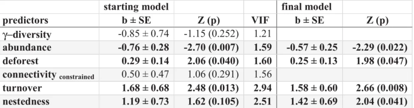
to assess the effects of stochastic processes on prevalence. In general, we found two main results. First, effect, generalized linear models (GLMs)
with α−diversity and γ−diversity
suggested that stochastic processes prevalence and diversity. Finally,
positively correlated with nestedness in
metacommunity, once that we accounted for stochastic processes represented b dispersal of species between communities.
Figure 1. Metacommunity framework used to investigate regiona Mycobacterium ulcerans. In this example, each of three regions (blue, red
encompasses two communities (
Regional prevalencei,j is influenced by regional diversity (
based processes driving dissimilarity between the t in two informative components: ordered loss of spec species between communities. Both, niche
increase the extent of nestedness between communiti regional MU prevalence
communities: probabilistic dispersal determined by (arrows) and the total abundance of animals in the
based processes dominated the assembly of lentic communitie assembly of lotic communities. Hence, we analysed t communities as two separated metacommunities, and examined the results as a pseud to assess the effects of stochastic processes on the relationship between
e found two main results. First, opposite to the prediction of the dilution generalized linear models (GLMs) revealed that MU prevalence was
diversity in the lotic metacommunity, but not in the lentic
processes may exert important effects on the relationship between Finally, as expected, we found that MU prevalence
positively correlated with nestedness in both, the lentic metacommunity we accounted for stochastic processes represented b dispersal of species between communities.
Metacommunity framework used to investigate regiona . In this example, each of three regions (blue, red encompasses two communities (i and j) with their respective local diversities (
is influenced by regional diversity (γi,j), and stochastic and niche
based processes driving dissimilarity between the two communities (βi,j).
in two informative components: ordered loss of species (nestedness) and turnover of species between communities. Both, niche-based and stochastic extinctions tends to increase the extent of nestedness between communities. Thus, we examine nestedness and
regional MU prevalencei,j while accounting for stochastic pro
communities: probabilistic dispersal determined by the connectivity between communities (arrows) and the total abundance of animals in the region, regardless the species.
ssembly of lentic communities whereas stochastic assembly of lotic communities. Hence, we analysed the lotic and lentic xamined the results as a pseudo-experiment the relationship between nestedness and MU opposite to the prediction of the dilution was positively correlated in the lentic one. This effects on the relationship between prevalence at regional level was metacommunity and in the lotic we accounted for stochastic processes represented by probabilistic
Metacommunity framework used to investigate regional prevalence of . In this example, each of three regions (blue, red, and yellow)
) with their respective local diversities (αi and αj).
), and stochastic and
niche-). βi,j is decomposed
tedness) and turnover of based and stochastic extinctions tends to es. Thus, we examine nestedness and while accounting for stochastic processes assembling the connectivity between communities region, regardless the species.
METHODS
MU is a relatively slow growing bacterium (~ 50h for replication) that synthetizes a lipophilic macrolide toxin (mycolactone), and evolved multiple DNA deletions and rearrangements associated with niche reduction (Stinear et al. 2007). Some works support the existence of vector-borne transmission and amplification by Belostomatidae and Naucoridae water bugs (Marsollier et al. 2003), and previous studies suggest that MU is embedded within ecological networks (Roche et al. 2013a). MU occurs on a wide diversity of substrata such as mud, organic detritus, biofilms on aquatic plants and in a large diversity of aquatic micro- and macro-invertebrates, fish, amphibians, reptiles and mammals (Portaels et al. 2001; Marsollier et al. 2004; Benbow et al. 2013; Willson et
al. 2013; Garchitorena et al. 2014; Morris et al. 2014).
Sampling and study sites
Periodic sampling of aquatic communities was performed in Akonolinga, Cameroon between June 2012 and May 2013. Monthly samples were collected in 16 aquatic communities within a region of
approximately 3,600 km2 including a wide spectrum of streams, rivers, swamps and flooded areas.
Sampling was performed during five consecutive days, and in each aquatic community four locations were chosen in areas of slow water flow and dominant aquatic vegetation. Classification of aquatic invertebrates was performed at the family level (see Garchitorena et al. 2014 for details).
Detection of M. ulcerans with qPCR
For each community and month sampled, the presence of MU was tested on 17 different taxonomic groups of animals (Garchitorena et al. 2014). However, not all of these groups were present across the study, and this may add variation in the presence of MU due to the differences across taxa in the affinity to harbour the bacterium (Portaels et al. 2001; Marsollier et al. 2004). To assure consistency in the sensitivity of detecting MU we focused on the orders of macro-invertebrates that were consistently present during the sampling year (Coleoptera, Diptera, Ephemeroptera, Hemiptera and Odonata, SM2). Quantitative PCR was used to detect two specific markers of MU in each sample: oligonucleotide primer and TaqMan probe sequences of IS2404 and the ketoreductase B domain of the mycolactone polyketide synthase (mls) gene from the plasmid pMUM001 (Garchitorena et al. 2014).
Probabilistic dispersal
Theory predicts that stochastic extinction of species in a community should decrease prevalence, as opposed to niche-based extinction of species that are expected to increase pathogen transmission (Ostfeld & LoGiudice 2003). Stochastic extinctions and colonisations of species in communities may occur due to probabilistic dispersal of species between neighbour communities (Connor & Simberloff 1979; Hubbell 2001; Chase & Myers 2011). In such instance, nearest communities are expected to be more similar than distant ones. Thus, we considered the connectivity between communities as surrogate of probabilistic dispersal, and accounted for its effects in our analyses in
three ways: First we assessed whether our data (local MU prevalence and α−diversity) were
structured by the connectivity between communities (SM3). Second, we included estimates of connectivity as predictors in the GLMs on regional MU prevalence (see below). Finally, because connectivity may interact synergistically with the other predictors of interest (i.e. nestedness and γ-diversity) we tested for two-way interactions between connectivity and the other predictors included in the GLMs on regional MU prevalence.
Connectivity between communities was represented by two estimates: Euclidean connectivity and constrained connectivity (SM3). Euclidean connectivity assumed that host and non-host species can disperse freely between communities across the landscape. Constrained connectivity assumed that species disperse within the hydrological system in Akonolinga. Connectivity was measured as the
inverse of distances between communities (Euclidean and constrained): , from (0) no
connectivity to (1) full connectivity. We present separate GLMs for each estimate of connectivity because including both estimates as predictors in the same GLM produced multicolinearity in the models.
Local analyses on MU prevalence
We performed GLMs to test the correlation between MU prevalence (the proportion of positive samples found during a year in each community) and α−diversity represented by the Shannon index
(H). The Shannon index was estimated as: ; where was the proportional
abundance of host species i and S was the total number of families in the community (Shannon 1948). Additionally, we considered two potential confounding effects that may influence MU prevalence: deforestation and total abundance of animals in the community, regardless the taxonomic group -henceforth abundance Deforestation is known to affect Buruli ulcer (Landier et