HAL Id: hal-00133172
https://hal.archives-ouvertes.fr/hal-00133172
Submitted on 1 Mar 2007
HAL is a multi-disciplinary open access
archive for the deposit and dissemination of sci-entific research documents, whether they are pub-lished or not. The documents may come from teaching and research institutions in France or abroad, or from public or private research centers.
L’archive ouverte pluridisciplinaire HAL, est destinée au dépôt et à la diffusion de documents scientifiques de niveau recherche, publiés ou non, émanant des établissements d’enseignement et de recherche français ou étrangers, des laboratoires publics ou privés.
A descriptive method to evaluate the number of regimes
in a switching autoregressive model
Madalina Olteanu
To cite this version:
Madalina Olteanu. A descriptive method to evaluate the number of regimes in a switching autore-gressive model. Neural Networks, Elsevier, 2006, 19, pp.963-972. �10.1016/j.neunet.2006.05.019�. �hal-00133172�
A Descriptive Method to Evaluate the Number of Regimes
in a Switching Autoregressive Model
Madalina Olteanu
SAMOS-MATISSE, University of Paris I 90 Rue de Tolbiac, 75013 Paris, France
madalina.olteanu@univ-paris1.fr
Abstract - This paper proposes a descriptive method for an open problem in time series analysis : determining the number of regimes in a switching autoregressive model. We will translate this problem into a classification one and define a criterion for clustering hierarchi-cally different model fittings. Finally, the method will be tested on simulated examples and real-life data.
Key words - switching autoregressive models, hierarchical clustering, Ward dis-tance, SOM
1
Introduction
In the past few years, several nonlinear autoregressive models were proposed for time series analysis. Some of these models are based on the idea that the process is characterized not by a unique linear autoregression, but by the fact that two or more regimes are driving the series behaviour. In each regime, an autoregressive function is fitted. We are interested in the case where the autoregressive functions are linear in every regime. The most classical examples are TAR (Treshold Autoregressive) models introduced by Tong (1978) with regime switching according to the magnitude of a treshold variable, the smoothed version of TAR models (STAR), or the more recent Markov switching autoregressive models, first used by Hamilton (1989) to model the U.S. Gross National Product.
Estimating the parameters of these models is usually done by maximizing the likelihood function, but under a very strong hypothesis, a fixed number of regimes. Choosing the “true” number of regimes is still an open problem, as this is equivalent to testing with lack of identifiability under the null hypothesis. This leads to a degenerated Fisher information matrix and thus the chi-square theory and the likelihood ratio tests fail to apply. An empirical method to detect this kind of non-linearity using Kohonen maps and hierarchical clustering of linear regressions is given below. The second section describes the method, while the third provides examples on simulated and real-life data. Finally, a conclusion will follow.
2
The Method
The problem of finding the “true” number of regimes can be rewritten as a classification problem by using a sliding window as follows . Suppose that we have observed the values of
a time series {yt}t=1,T and we decide to fit an autoregressive model. Once the order of the
model has been determined (with an AIC criterion, for example), we can consider the data set of dimension (T − p)x(p + 1), {yt, yt−1, ...yt−p}t=p+1,T. Looking for the number of regimes
is actually equivalent to looking for the number of regression lines (or hyperplanes) which will best fit the data.
The idea is simple and is based on the possibility of finding patterns in data which will identify the regression hyperplanes. Given the data set in Figure 1, fitting one regression line to the data is clearly not the good choice. If we now suppose that we managed to cluster the data into two groups and we perform a regression within each of these groups, we get two lines which seem to describe better the sample. This is confirmed by the “within squared error”, which is equal to the sum of squared residuals if there is only one regime and, if there are several, to the total sum of squared residuals within each group.
2.0 2.5 3.0 3.5 4.0 0.0 0.5 1.0 1.5 2.0 x y 2.0 2.5 3.0 3.5 4.0 0.0 0.5 1.0 1.5 2.0 x y
Figure 1: Fitting clustered data
In the general case, we would like to start with some “good” initial clusters which will be then classified hierarchically using some squared error criterion and we would expect to have an important break in the increasing values of this criterion, once we pass from the true number of regimes to a smaller one.A “good” cluster should contain observations belonging to the same regime and, at the same time, have enough points to estimate a regression line.
2.1 Initial clustering
For the initial clustering, self-organizing maps were employed. This choice was motivated by several properties of the Kohonen maps such as the vector quantization property (the last steps of the algorithm use “0-neighbours”and thus are equivalent to classical VQ tech-niques), the homogeneity of the clusters as well as the topology conservation used to fasten the hierarchical classification algorithm.
One problem arises once we get the clusters and try to fit a regression within each one : are there enough points in every cluster? No cluster will be allowed to have less points than the number of lags or regressor variables. For this, either we eliminate from the analysis those which do not verify this condition, either we force the points to move to a different cluster, by assigning them to the closest sufficiently large cluster.Since very few observations are concerned with this problem and in order to shorten the computing time, the first approach was preferred.
The assumption we make here is that the property of homogeneity of self-organizing maps manages to create clusters in which observations belong to one regime. This could be justified by the fact that the variables used for the classification contain information concerning the regime of the observation and similar profiles will belong to the same cluster. Indeed, in the simulated examples where the different regimes are known, we’ll see that the map clusters are generally homogeneous from this point of view. This property will no longer apply if the regression hyperplanes are too close and the noise is important.
2.2 Hierarchical classification
As we actually need to compare different data fits, which is also equivalent to different numbers of hyperplanes, we need to adapt a hierarchical classification to our case (let us first make the convention to call “clusters” the result of the Kohonen map and “classes” two or more “clusters” joined together by the hierarchical method). We will choose a new “distance” between classes by developping a squared error criterion.
A very popular method used in classification is to minimize a within-class variation criterion, the variation within a class being defined as the sum of squared distances from the individuals to the barrycenter. By considering a data set xi ∈ Rn, i = 1, ..., N and a fixed number of
clusters k, the total within-class variation can be written as Iw =Pki=1wiIi , where wi is the
weight of class i, Ii = PNj=1i d2(xi,j, gi) being the variation within the class i and gi is the
corresponding barrycenter. We denoted by Ni the number of individuals in class i and by
xi,j the data point indexed by j in class i.
In hierarchical classification, this principle was adapted by Ward and the algorithm consists in clustering together the individuals who minimize the increase of the within-class variation. Our idea was to build an algorithm similar to Ward’s, but, as our interest is to estimate the number of hyperplanes characterizing the data, we will replace the barrycenters by regression lines and the within-class variation becomes the within sum of squared errors. Obviously, in this case, the inter-class variation cannot be defined.
For a fixed number of classes, k, the within sum of squared errors is defined as SSEw,k=Pkl=1SSECl,
where SSECl =
P
t∈Cl(yt− ˆyt)
2 is the sum of squared residuals and ˆy
t is the predicted value
of yt by the linear regression of order p fitted in class Cl, l = 1, k.
Now, in the frame of hierarchical clustering, when passing from k to k − 1 classes, if classes iand j were clustered, the within sum of squared errors becomes :
SSEw,k−1i,j =Pk
l=1,l6=i,l6=jSSECl+ SSECi∪Cj
Following the same principle as Ward’s, we want to minimize the increase in the within inertia, which in this case is defined by the within sum of squared errors. This is equivalent to finding i and j which minimize
∆Sw,k,k−1i,j = SSEw,k−1i,j − SSEw,k= SSECi∪Cj− SSECi− SSECj
2.2.1 The within sum of squared errors criterion
Now, let us take a closer look at this difference and give an explicit expression as a function of the data and the residuals. The following notations are necessary :
- Yi = {Yt}t∈Ci ∈ R
ni, Y
j = {Yt}t∈Cj ∈ R
nj, where n
i and ni are the cardinalities of Ci and,
respectively, Cj
- Xi = {1, Yt−1, ..., Yt−p}t∈Ci ∈ Rni×(p+1), Xj = {1, Yt−1, ..., Yt−p}t∈Cj ∈ Rnj×(p+1).
The linear regressions fitted in classes Ci and Cj can be written as :
Yi= Xi· βi+ ui= Xi· ˆβi+ ei
Yj = Xj · βj+ uj = Xj· ˆβj+ ej,
where βi, βj, ˆβi, ˆβj ∈ Rp+1, ˆβi and ˆβj are the least squares estimates of βi and βj, ui, ei ∈ Rni
and uj, ej ∈ Rnj are the error and, respectively, the residuals vectors, ui ∼ N (0, σi2Ini) and
uj ∼ N (0, σ2jInj).
The linear regression fitted in the joint class Ci∪ Cj is written as :
Y = X · β + u = X · ˆβ+ e, where Y = · Yi Yj ¸ ∈ Rni+nj, X = · Xi Xj ¸ ∈ R(ni+nj)×(p+1),
β, ˆβ ∈ Rp+1, ˆβ is the least squares estimate of β, u, e ∈ Rni+nj are the error and the residuals
vector and u ∼ N (0, Ω), Ω = µ σ2iIni 0 0 σj2Inj ¶ . Then, we can compute ∆Sw,k,k−1i,j as :
• ∆Sw,k,k−1i,j = SSECi∪Cj− SSECi− SSECj = e0e − (ei0ei+ ej0ej)
Remark 1 :
Using this form, Toyoda (1974) proves that ∆Sw,k,k−1i,j is approximately distributed as σ2χ2(p + 1), where σ2 is any well-chosen weighted average of σ2i and σj2 and p is the number of lags con-sidered.
• ∆Sw,k,k−1i,j = SSECi∪Cj−SSECi−SSECj =
° ° °Y − X · ˆβ ° ° ° 2 −°° °Yi− Xi· ˆβi ° ° ° 2 −°° °Yj− Xj· ˆβj ° ° ° 2 (1) But Y − X · ˆβ = · Yi− Xi· ˆβ Yj− Xj· ˆβ ¸ = · Yi− Xi· ˆβi Yj− Xj· ˆβj ¸ + · Xi· ˆβi−Xi· ˆβ Xj· ˆβj− Xj· ˆβ ¸ (2) and thus ° ° °Y − X · ˆβ ° ° ° 2 = ° ° ° ° Yi− Xi· ˆβ Yj− Xj· ˆβ ° ° ° ° 2 = ° ° ° ° Yi− Xi· ˆβi Yj− Xj · ˆβj ° ° ° ° 2 + ° ° ° ° Xi· ˆβi−Xi· ˆβ Xj · ˆβj− Xj· ˆβ ° ° ° ° 2
since the cross-product on the right term in (2) can easily be seen to be zero. We get that : ° ° °Y − X · ˆβ ° ° ° 2 = ° ° °Yi− Xi· ˆβi ° ° ° 2 + ° ° °Yj− Xj· ˆβj ° ° ° 2 + ° ° °Xi· ˆβi−Xi· ˆβ ° ° ° 2 + ° ° °Xj· ˆβj − Xj · ˆβ ° ° ° 2 (3) and by replacing (3) in (1) : ∆Sw,k,k−1i,j =°° °Xi· ˆβi−Xi· ˆβ ° ° ° 2 +°° °Xj· ˆβj − Xj· ˆβ ° ° ° 2 = = ( ˆβi− ˆβ)0Xi0Xi( ˆβi− ˆβ) + ( ˆβj − ˆβ)0Xj0Xj( ˆβj − ˆβ) (4)
Using the form of the least squares estimators ˆβi, ˆβj and ˆβ
ˆ βi− ˆβ = βi− β + nh (Xi0Xi)−1Xi0, 0 i − (Xi0Xi+ Xj0Xj)−1[Xi0, Xj0] o · · ei ej ¸
ˆ βj− ˆβ = βj− β + nh 0, (Xj0Xj)−1Xj0 i − (Xi0Xi+ Xj0Xj)−1[Xi0, Xj0] o · · ei ej ¸ and (4) becomes ∆Sw,k,k−1i,j = (βi− β)0Xi0Xi(βi− β) + (βj − β)0Xj0Xj(βj− β)+ +(βi− β)0 n Xi0ei− Xi0Xi(Xi0Xi+ Xj0Xj)−1(Xi0ei+ Xj0ej) o + +nei0Xi− (ei0Xi+ ej0Xj) (Xi0Xi+ Xj0Xj)−1Xi0Xi o (βi− β)+ +(βj− β)0 n Xj0ej− Xj0Xj(Xi0Xi+ Xj0Xj)−1(Xi0ei+ Xj0ej) o + +nej0Xj− (ei0Xi+ ej0Xj) (Xi0Xi+ Xj0Xj)−1Xj0Xj o (βj− β)+ +ei0Xi(Xi0Xi)−1Xi0ei+ ej0Xj(Xj0Xj)−1Xj0ej− − (ei0Xi+ ej0Xj) (Xi0Xi+ Xj0Xj)−1(Xi0ei+ Xj0ej)
If classes i and j come form the same regime, that is βi = βj = β, the increase in the within
sum of sqared errors is only
∆Sw,k,k−1i,j = ei0Xi(Xi0Xi)−1Xi0ei+ ej0Xj(Xj0Xj)−1Xj0ej−
− (ei0Xi+ ej0Xj) (Xi0Xi+ Xj0Xj)−1(Xi0ei+ Xj0ej)
This quantity is very close to zero if the classes contain enough points. Thus, together with remark 1,we get that if the joint classes are from the same regime, the within sum of squared errors should be close to zero and if the classes are from different regimes, the larger the difference between the parameters of the two regimes, the increase in the within sum of squared errors should be larger.
2.3 The algorithm
Now, we can write the steps of the algorithm which, at the same time, clusters the data and models the dependencies within each class:
We consider k going from M to 2, where M is the number of clusters resulting from the Kohonen map.
For each k, we have the following steps :
• Compute the k regressions lines corresponding to the k classes • Find (i0, j0) which minimize ∆i,jSSEw
• Join these classes together, put k = k − 1 and go to the first step.
At the last step all points are clustered together and there is a single regression line.
The next thing to do is draw the dendrogram and look how the within sum of squared errors increases over the classification. As it was mentioned earlier, one might expect an important break when the number of classes is smaller than the real number of regimes.
Regime1 Regime2
Intercept yt−1 yt−2 Intercept yt−1 yt−2
value -2.82 0.59 -0.89 1.4 0.37 0.32
t-value -19.15 13.09 15.89 8.24 5.96 4.79
Table 1: Coefficients for the TAR model
3
Examples and Results
The method was tested on several nonlinear autoregressive regime switching models. Histor-ically, the first introduced were the treshold models (we won’t speak here about the other variants of these models, smoothed etc), followed by the switching Markov and next we will consider both examples.
3.1 TAR Models
The example is a TAR of order two and the coefficients were taken from the paper of Gon-zalo&Pitarkis. yt= ½ −3 + 0.5yt−1− 0.9yt−2+ εt 2 + 0.3yt−1+ 0.2yt−2+ εt , yt−2 ≤ 1.5
, yt−2 >1.5 , where {yt} is the observed series and εtis
i.i.d. standard gaussian.
Three samples containing 200, 400 and 800 points, respectively, were simulated. Let us examine the 200 points sample. The self-organizing map dimension was fixed equal to 5x5 and {yt, yt−1, yt−2} were the variables used for the classification. Crossing the map with a
boolean variable which distinguishes whether yt−2 is above or below the treshold value allows
to see that the clusters are homogeneous and each of them takes values in one regime. If the hierarchical clustering algorithm is run on the twenty-five clusters, the squared error criterion increases as in Figure 3 and suggests that a good choice would be a two-regimes model. The hierarchical classification provides also good estimators for the parameters of the model when choosing two regimes as shown in Table 1.
The threshold value was not estimated and we’ll see that the decision on the type of the model (TAR, Markov switching) cannot be made on this basis only.
Figure 2: Initial clustering with a Kohonen map for TAR model
When increasing the number of points in the sample, we have chosen to increase also the map size (we considered a 7x7 map for the 400 sample and a 9x9 for the 800). This was done in
5 10 15 20 200 400 600 800 1000 1200 Number of clusters MSE
Figure 3: Squared error criterion for TAR model
the purpose of conserving clusters homogeneity, but a good criterion for choosing the size of the map is still to be defined. The results are very similar and in both cases the hierarchical algorithm suggests a two-regimes model.
3.2 A Two Regime Markov Switching Model
For this example, we will first define an autoregressive Markov switching process. If {yt}t∈N
is the observed time series, let us suppose that it follows a linear autoregressive process of order p and that we have two regimes, the passage from one regime to the other being driven by an unobserved Markov chain, {xt}t∈N, which has a transition probability matrix A.
For two regimes and two lags of time, we can write the model as follows : yt= fxt(yt−1, yt−2)+
σxtεt
fxt(yt−1, yt−2) ∈ {f1, f2}, σxt ∈ {σ1, σ2}, εt i.i.d. noise (usually a standard gaussian) and
A=
µ
p 1 − p
1 − q q
is the transition probability matrix of xt.
The data used here were simulated with the parameters below (a globally stationary process was chosen): ½ f1(yt−1, yt−2) = 0.2 + 0.5yt−1+ 0.1yt−2 f2(yt−1, yt−2) = 0.3 + 0.9yt−1− 0.1yt−2 , ½ σ1= 0.03 σ2= 0.02 and A = µ 0.9 0.1 0.2 0.8 
As for the previous example, three samples (200, 400, 800 points) were considered. We will only list the results for the 400 sample and remark that the outputs for the other two cases were very similar. The initial clustering was performed using a 6x6 Kohonen map and {yt, yt−1, yt−2}as variables. Figure 4 shows that the map is well organized, the clusters
are homogeneous and when crossing with the variable giving the regime, there is a good separation of them in the initial clusters.
Afterwards, from the hierarchical classification of these clusters, we get, again, a huge jump when passing from two classes to one, as shown in Figure 5.The estimated coefficients in each of the two classes are shown in Table 2 (we will also note that the two clusters are homogeneous, the pourcentage of explained variance being larger than 92% in each of them).
Figure 4: Initial clustering with a Kohonen map for two regimes Markov 0 5 10 15 20 25 30 1 2 3 4 Number of clusters MSE
Figure 5: Squared error criterion for 2 regime Markov
Regime1 Regime2
Intercept yt−1 yt−2 Intercept yt−1 yt−2
value 0.3 0.88 -0.09 0.18 0.39 0.24
t-value 41.56 32.89 -3.64 20.91 12.07 8.87
Table 2: Coefficients for the two regime Markov model
3.3 A Three Regime Markov Switching Model
Now let us see what happens if we add a new regime to the model, which will moreover be explosive and drive the process into a nonstationary one. The following example was considered :
yt = fxt(yt−1, yt−2) + σxtεt , fxt(yt−1, yt−2) ∈ {f1, f2, f3}, σxt ∈ {σ1, σ2, σ3}, εt is i.i.d.
standard gaussian and f1(yt−1, yt−2) = 0.2 + 0.5yt−1+ 0.1yt−2 f2(yt−1, yt−2) = 0.3 + 0.9yt−1− 0.1yt−2 f3(yt−1, yt−2) = 0.5 + 1.2yt−1+ 0.5yt−2 , σ1 = 0.03 σ2 = 0.02 σ1 = 0.03 and A = 0.8 0.1 0.1 0.1 0.8 0.1 0.6 0.2 0.2
The following results are from a 400 points sample, with an initial 8x8 map. By crossing the map with the regime variable, there is a relatively good separation, although we may notice that the first two regimes seem to come closer together with respect to the third one. Here, a first conclusion would be that there are four regimes. But let us take a closer look at the hierarchical classification. One of the four final classes contains only one cluster, one cell of the map. Moreover, this cell (the 8th) is isolated from the rest of the map and it contains only four observations with very high values. If we project the data on a two or
Figure 6: Initial clustering with a Kohonen map 0 10 20 30 40 0 20 40 60 80 Number of clusters MSE
Figure 7: Squared error criterion for 3 regimes Markov
three-dimensional space, the same four observations are far from the rest. The algorithm has identified a small class of outliers which are considered as a separate regime and from this point of view the method is close to Ward’s which is also sensitive to this kind of observations. We can’t continue with the examples before making an important remark. We’ve seen that this method of identifying the number of regression lines works quite good in the examples above. Concerning the parameter estimation and making a decision about the model (TAR or Markov switching?, for instance), the hierarchical classification provides only the estimators for the regression lines, a likelihood approach should be used instead, once we fixed the number of regimes, to estimate the rest of the parameters : threshold value, transition matrix etc. As for the second question, no theoretical result is available yet, the econometricians preferring to decide on other criteria (economic, social etc).
3.4 What about Real Life Data?
The results on the simulated examples being encouraging, we decided to run the algorithm on real data sets. Three examples were chosen, the first two are the benchmarks Old Faithful Geyser Data and Santa Fe Competition Laser Data and the third is the U.S. GNP (Gross National Product) series, used by Hamilton to introduce the switching Markov models.
3.4.1 Old Faithful Data
The first set of data is the classical Old Faithful Geyser in Yellowstone National Park, con-sisting of 299 pairs of measurements referring to the waiting time between two successive eruptions, wt, and the duration of the subsequent eruption, dt. The data was collected
be-tween August 1st and August 15th, 1985 and the two variables are recorded in minutes. Several studies of this sample are available, most authors trying to assess either the cluster-ing of the data, either the dependency between successive events. A literature overview, as well as an analysis using time series while assuming “a priori” the existence of two patterns of dependency, can be found in Azzalini and Bowman (1990) paper. Although there are no autoregressors in this case, the problem is the same : find the number of clusters and fit a regression within each one.
Our approach would be to detect the clustering of the data and, at the same time, model the dependency within each class. The idea of addressing clustering and dependency at the same time was firstly introduced by Hennig (2000) who uses regression fixed point clusters. Here, the duration of the eruption was modeled as a linear function of the waiting time before the eruption. While plotting the duration against the waiting time, one can see that there are at least two clusters of points, depending on the waiting time. Let us make one last remark on the data, which is that due to inexact observations during the night, there are 53 points with duration=4 (long eruption) and 20 with duration=2 (short eruption). The medium eruptions (duration=3) appear only once.
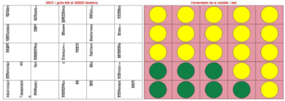
For the Kohonen classification the data set {wt, dt}t=1,299 was considered (no lags of time
were introduced). The map was chosen to be a 6x6 grid and 1000 iterations were performed. Afterwards, an hierarchical clustering minimizing the within sum of squared errors criterion was applied to the 33 “valid” clusters (one cluster was void and two others contained only one point).
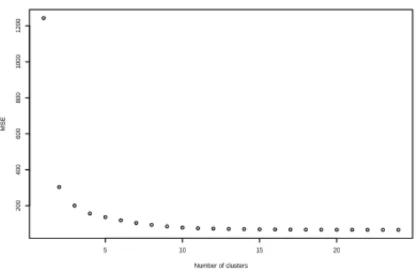
In Figure 8, the within sum of squared errors as well as the difference ∆SSEk,k−1are plotted.
The heterogeneity of the data is obvious and one can see that at least two clusters should be considered. On the contrary, passing from three clusters to two is less obvious and we shall see next that there’s overlapping of the clusters and that the regression coefficients are very close. 0 5 10 15 20 25 30 0 50 100 150 200 No of classes
Sum of squared errors
0 5 10 15 20 25 30 0 50 100 150 200 No of classes
Sum of squared errors difference
Figure 8: Squared error criterion for the old faithful data
Once we get the hierarchical classification, we get back to the self-organizing map to see how the classes spread over the grid. On the first graph in Figure 9, the tree-cut at two classes
in presented : the first class in the right upper corner in light-grey circles and the second beyond the diagonal of the grid in dark-grey circles. Clusters 7 and 28 do not contain enough points and were not considered in the classification.
Figure 9: The self-organizing map for the old faithful data
While the 2-classes model is meaningful, in the 3-classes case things seem to be more com-plicated : the first class is the same, well isolated in the right upper part of the grid, while classes 2 and 3 are mixed on the grid. This is even more obvious if we plot the duration dt
against the waiting time wtand identify the classes as shown in Figure 10.
40 60 80 100 0 1 2 3 4 5 6 Waiting Duration 40 60 80 100 0 1 2 3 4 5 6 Waiting Duration
Figure 10: 2-clusters and 3-clusters of the old faithful data
The same situation as for the Kohonen map occurs. In both cases, 2-classes and 3-classes model, a first class (the right upper part of the self-organizing map) is well isolated from the rest and is concentrated around the waiting=2 points. This class corresponds to short time eruptions preceeded by rather long waiting times. The second class on the first graph containts all the long duration points including all duration=4 points. This class is splitted into two when considering the 3-classes case : one sub-class is formed by the duration=4 points and the long time erruptions preceeded by long waiting times, while the second contains the data with a moderately decreasing tendency in the duration for increasing waiting times. Although there is an interpretation for the 3-classes model, the within squared error criterion used for the classification suggests a 2-classes model, because it corresponds to an important break in the increase of the squared error. Besides, in the discussion of Azzalini and Bowman
(1990) geological evidence for the existence of two distinct patterns of eruptions is given and thus our conclusion is enhanced.
3.4.2 Santa Fe Competition Laser Series
For the laser series, a highly nonlinear data set, the algorithm selects three classes as shown in Figure 11. In order to compare the results with the existing literature, ten lags of time were used. The 10000 observations were initially clustered on a 9x9 map. Once the number of regimes was fixed, the three regimes were supposed to be the states of a discrete Markov chain and the parameters were estimated using the EM algorithm as described in Rynkiewicz (1999). The prediction results are weaker than those obtained by Weigend (1995) or Rynkiewicz (1999), but the number of estimated parameters is much smaller. But, as the nonlinearities of the series are not entirely explained by a mixture of linear regressions, an adaptation of the method by replacing the linear functions with nonlinear ones could be more interesting for this kind of data.
0 20 40 60 80 0 e+00 1 e+06 2 e+06 3 e+06 4 e+06
Figure 11: Squared error criterion for the laser series
3.4.3 GNP Series
Concerning the GNP series, Hamilton’s approach was based on the assumption that the mean growth rate is subject to occasional, discrete shifts. We dispose of 136 trimestrial observed values of the series, from 1952 until 1984. The maximal lag to be considered was determined with the AIC criterion and was fixed at p = 3.
The data was initially clustered with a 4x4 map and considering {yt, yt−1, yt−2, yt−3} as
variables. The sixteen clusters were grouped hierarchically by the squared error criterion and the results are displayed in Figure 12.
The first graph contains the within sum of squared errors plotted against the number of classes and the sencond its percentage increase. A first break appears when considering six classes instead of seven, but this can be interpreted as being due to possible stronlgy homogeneous clusters from the same regime which get mixed. There is a second break(13%) when passing from two classes to one but this is less obvious than in previous cases and the decision to model this series by a two-regime model is questionable from our point of view.
2 4 6 8 10 12 50000 55000 60000 65000 70000 75000 Number of clusters MSE 2 4 6 8 10 12 0 2 4 6 8 10 12 Number of clusters % increase
Figure 12: Squared error criterion for GNP data
4
Conclusion and Future Work
We’ve introduced a descriptive method to assess the presence of regime changes in nonlinear time series analysis. As there is no theoretical answer and no statistical test to solve this problem for the moment, this method may be used, but with precaution. Indeed, self orga-nizing maps could mix the regimes if the regression hyperplanes are too close and the square error criterion seems to be sensitive to outliers.
Thus, several improvements should be made in the future, like considering a different distance that would take into account the temporal dependency of the data for the initial clustering or like looking for a smarter initial clustering that would avoid mixing regimes in the same cluster. Replacing the linear regressors by nonlinear functions could also be a possibility, but then the number of parameters becomes larger and the fiability of the estimators decreases.
References
[1] Azzalini A., Bowman A.W. (1990), A Look at Some Data on the Old Faithful Geyser, Applied Statistics, vol. 39 p. 357-365.
[2] Chow G.C. (1960), Tests of Equality Between Sets of Coefficients in Two Linear Regres-sions, Econometrica, vol. 28 p. 591-605.
[3] Gonzalo J., Pitarakis J-Y. (2002), Estimation and Model Selection Based Inference in Single and Multiple Treshold Models, Journal of Econometrics, vol. 110 p. 319-352. [4] Hamilton J.D. (1989), New Approach to the Economic Analysis of Nonstationary Time
Series and the Business Cycle, Econometrica, vol. 57 p. 357-384.
[5] Hennig C. (2000), Regression Fixed Point Clusters : Motivation, Consistency and Sim-ulations, Preprint 2000-02, Fachbereich Mathematik, Universitat Hamburg
[6] Kohonen T. (1997), Self-Organizing Maps, New-York, Springer-Verlag.
[7] Letremy P. (2000), Notice d’installation et d’utilisation de programmes bases sur l’algorithme de Kohonen et dedies a l’analyse des donnees, Prepub. Samos 131.
[8] Rynkiewicz J.(1999), Hybrid HMM/MLP Models for Time Series Prediction, ESANN’1999 Proceedings, p. 455-462.
[9] Tong H. (1978), On a treshold model, Pattern Recognition and Signal Processing, ed C.H. Chen, Amsterdam : Sijhoff&Noordhoff.
[10] Toyoda T. (1974), Use of the Chow Test under Heteroscedasticity, Econometrica, vol. 42p. 601-608.
[11] Weigend A.S., Mangeas M., Srivastava A.N.(1995), Nonlinear gated experts for time series : discovering regimes and avoiding overfitting, International Journal of Neural Systems, vol. 6 p. 373-399.