HAL Id: hal-01441543
https://hal.archives-ouvertes.fr/hal-01441543
Submitted on 19 Jan 2017
HAL is a multi-disciplinary open access
archive for the deposit and dissemination of
sci-entific research documents, whether they are
pub-lished or not. The documents may come from
teaching and research institutions in France or
abroad, or from public or private research centers.
L’archive ouverte pluridisciplinaire HAL, est
destinée au dépôt et à la diffusion de documents
scientifiques de niveau recherche, publiés ou non,
émanant des établissements d’enseignement et de
recherche français ou étrangers, des laboratoires
publics ou privés.
the Analysis of Modal Distributions Obtained by FEM
Gerard Orjubin, Elodie Richalot, Odile Picon, Olivier Legrand
To cite this version:
Gerard Orjubin, Elodie Richalot, Odile Picon, Olivier Legrand. Chaoticity of a Reverberation
Cham-ber Assessed From the Analysis of Modal Distributions Obtained by FEM. IEEE Transactions on
Elec-tromagnetic Compatibility, Institute of Electrical and Electronics Engineers, 2007, 49 (4), pp.762-771.
�10.1109/TEMC.2007.908266�. �hal-01441543�
Abstract--. Wave chaos theory is used to study a modeled
reverberation chamber (RC). The first 200 modes of an RC at a given stirrer position are determined by the finite element method, and the Weyl formula is checked for various RC geometries, from integrable to chaotic. The eigenfrequency spacing distribution varies according to the degree of ray chaos in the RC related to its geometry. The eigenmode distributions are also analyzed and compared to the theoretical Gaussian distribution: close to the lower useable frequency, the modes of the studied chaotic RC fairly respect this asymptotic property. A general result of chaotic systems is illustrated: when perturbed by the stirrer rotation, the resonant frequencies of an RC avoid crossing. This means that the frequency sweeps tend to vanish at high frequency.
Index Terms— Eigenvalue perturbation, finite element method,
quantum chaos, reverberation chamber.
I. INTRODUCTION
n the last decade, reverberation chambers (RCs) have been increasingly used for electromagnetic compatibility tests. The behavior of an electrically large RC can be easily explained by the ray propagation approach: on the basis that the electric field is a superposition of an infinite number of uncorrelated and isotropic plane waves reflected by the walls, the field is isotropic and uniform [1].
Using this geometric optic point of view, Cappetta [2] has illustrated the chaotic behavior of an RC with a moving wall. In this paper, the chaotic behavior of a cavity equipped with a metallic stirrer will be discussed making use of quantum chaos theory.
Quantum chaos (or wave chaos) theory is nowadays frequently validated by microwave experiments in metallic cavities: the analogy between the Schrödinger and Helmholtz
This work was partially supported by the Brazilian agency CNPq.
G. Orjubin is with Laboratório de Telecomunicações e Ciência e Engenharia dos Materiais (LOCEM), Universidade Federal do Ceará, Fortaleza, 60455-760, Ceará, Brazil (e-mail: orjubin@univ-mlv.fr).
E. Richalot and O. Picon are with Equipe Systèmes de Communications et Microsystèmes (ESYCOM) Laboratory, Université de Marne-la-Vallée, 77454 Champs sur Marne, France (e-mail: elodie.richalot@univ-mlv.fr; odile.picon@univ-mlv.fr).
O. Legrand is with Laboratoire de Physique de la Matière Condensée, Université de Nice-Sophia Antipolis, Parc Valrose, 06108 Nice cedex 2 France (email: olivier.legrand@unice.fr)
equations is total in the case of a flat metallic cavity [3-5], and the results [6-7] prove that 3-D electromagnetic problems are compatible with the universal laws of quantum chaos theory. A law is said to be universal if it depends only on the system symmetry, but not on the geometrical details.
This paper presents an application of the quantum chaos theory to a modeled RC with the objective to study the pertinence of the universal laws for this particular 3-D electromagnetic problem. Another particularity lies in the restricted number of studied modes, whereas the theory applies to a large number of modes.
The RC chaoticity can be assessed from the statistics of the eigenfrequencies that are numerically determined by the finite element method (FEM). The considerable computational effort, which had been pointed out by Bunting in [8], can now be overcome [9] due to progresses in solver algorithms and hardware. It is worth noting that this work only concerns the modes, with neither consideration about the total electric field nor the quality factor, and that the main part of the paper is devoted to the RC analysis for a given stirrer position.
The outline of this paper is the following. First, we present the rationale for the use of quantum chaos theory [10] and we explain how the frequency distribution can be used to assess the RC chaoticity. This technique is then applied to three different kinds of RC, from integrable to chaotic ones. As well the eigenfield distributions are compared to the theoretical predictions in the integrable and chaotic cases.
In the last section, an important property of chaotic systems is presented, relative to the perturbation of resonant frequencies by the stirrer displacement. This study is conducted using a specific mode tracking procedure (MTP) [11].
II. THEORETICAL BACKGROUND
A. Quantum Mechanics and Microwave Studies
The analogy between Schrödinger and Helmholtz equations justifies the use of quantum mechanics theory to analyze the electromagnetic field inside a flat cavity. To show it, we recall the time-independent Schrödinger equation of a quantum
Chaoticity of a Reverberation Chamber
Assessed From the Analysis of Modal
Distributions obtained by FEM
G. Orjubin
1, E. Richalot
2, O. Picon
2,
and O. Legrand
3mechanical system described by the wave function ψ of a particle of mass m and energy E:
0
2
2 2+
=
∇
ψ
ψ
h
E
m
, (1)where
h
is the Planck constant. When the particle is inside a box, the boundary conditions are ψ = 0 on the frontiers.Quantum theory is validated from numerical simulations or experiments. In recent years, microwave analog experiments have become a well-established alternative to theoretical studies. The first 2D experiments were made with a flat cavity parallel to the plane Oxy for which the Helmholtz equation for the component Ez is
0
2
2 2
=
+
∇
E
zE
zλ
π
, (2)where λ is the wavelength of the harmonic wave. Equations (1-2) reveal the one-to-one correspondence between the two applications.
The validation technique consists in finding the resonant frequencies of a cavity from the transmission coefficient between two antennas [3-5][12]. Then the eigenfrequency distributions are analyzed with regard to the universal laws predicted by quantum chaos theory.
It is important to note that the extension of quantum techniques to 3-D electromagnetic cavities is not obvious, since the Helmholtz equation is vectorial, and is not equivalent to the Schrödinger equation. However, recent studies [6-7] prove that the universal laws are still valid for 3D electromagnetic cavities.
B. Semiclassical Mechanics and Geometric Optics
The properties of quantum systems that will be considered in Sections II-E and F are related to the chaotic dynamics of a particle free to move inside a box, in the classical limit where the de Broglie’s wavelength is vanishing small compared to the typical size of the box. In the electromagnetic context, the analogue limit is the geometrical imit of rays that are reflected by the metallic walls of the cavity. The reader is referred to [13] for a review of results on time-harmonic wave propagation in a ray chaotic enclosure. It is explained that a system with separable geometry (such as a rectangular cavity) is said to be integrable and has a regular behavior, to be opposed to chaotic systems.
On the basis of the close connection existing between ray and modal spectral properties, this paper will show how to use the modes of an RC to determine its degree of chaos.
C. Eigenfield Distribution in a Chaotic RC
As indicated in [13], the scalar eigenfunction ψ of a quantum system can be written as a superposition of plane waves (rays) with fixed wave vector amplitude. If the system is integrable, the number of these waves is limited (e.g. 8 plane waves for a 3-D rectangular cavity). For a chaotic system, the number is large and the propagation directions are uniformly distributed:
this is the random plane wave omdel introduced by Berry [14] for quatum mechanics and by hill [1] in the RC context. Applying the central limit theorem to this conjecture, one can deduce that ψ follows a Gaussian distribution for almost2 all modes. As the eigenfields are real, their squared amplitudes fallow a Porter-Thomas distribution [10].
The experimental verification using 3D electromagnetic cavities shows that the first few hundred eigenfields seem to conform to that normal distribution [6-7]. It must be noted that this result is valid only for points distant from the walls by at least roughly a quarter of wavelength [7].
In the RC case, the normality of the eigenfield distributions implies that each squared rectangular component of the complex2 field is exponentially distributed, when evaluated over a stirrer rotation. This is one of the so-called asymptotic laws valid for chaotic RCs. The RC chaotic behavior may come from the stirrer presence, the corrugated walls, the cavity irregularities, or the cavity shape. As an illustration, a generalization of the 2-D Bunimovich stadium to a 3-D structure with moving corrugated walls has been proposed as an RC geometry [16].
D. Weyl Formula
Much of the techniques used in quantum chaos are related to the study of the eigenvalues, i. e. the resonant frequencies of the cavity. Balian and Bloch [17] have treated theoretically the distribution of electromagnetic eigenmodes in a cavity with perfectly conducting walls. Using the notation of Arnaut [18], the expression for the averaged modal density as a function of the frequency f is + − = −2 2 8 c f o c c f c V df dN avg
κ
π
, (3)where c is the light speed in vacuum, V is the cavity volume and the geometric dependent constant κ is defined by
( )
( )
( )
( )
∫
−∫
− − = S L dl r r r r d r r r rϕ
ϕ
π
ϕ
π
π
ρ
σ
π
κ
( )( 5 ) 6 1 3 4 , (4)where S is the cavity surface, L is the edges length, and the
( )
[
1 1]
12
−+
− −=
ρ
θρ
ϕρ
r
r
is the averaged radius of curvature of surface element dσ at r for spherical angles θ and φ. Functionϕ
( )
r
r
is the local dihedral internal angle along edge dl.We can emphasize two main properties. First, at high frequency, the dominant term of (3) does not depend on κ: the average modal density is then independent of the RC surface. The integration of (3) leads to the approximate Weyl formula
2 Deviations from this universal law may concern localized modes associated to short unstable (“scarred eigenfunctions”) [4] orto non-isolated marginally-unstableperiodic orbits (“bouncing-ball modes”) [15].
2 Applying a perturbation technique to low losses enclosures leads to a
of the cumulative number of modes N(f) below a given frequency f: 3 3 8 ) ( ≅ c f V f N avg
π
. (5)As a second property, we note that the formula (3) is the same for chaotic or non chaotic systems. The difference between these two kinds of system is embedded within the local fluctuations of the modal density. This point is presented in §IIF.
E. Random Matrix Theory
According to accepted conjectures3, generic chaotic systems follow the universal laws predicted by the random matrix theory (RMT) [10]. In RMT the linear wave equation (1) is replaced by a linear matrix equation where the elements of the matrix are random variables. The matrix statistics are those that would result if the matrix were drawn from different types of ensembles, where the relevant ensemble type depends only on the underlying symmetry of the system. The ensemble that is relevant to lossless electromagnetic problems is the Gaussian orthogonal ensemble (GOE) as GOE is generally suited to describe chaotic system with time reversal symmetry. To describe a lossless integrable system, the Poissonian orthogonal ensemble (POE) must be used.
We will see in the next paragraph that, depending on the RC general property (chaotic or not), the distribution of the resonant frequencies is obtained from the GOE or POE hypothesis. Although RMT supposes that the number of modes to be analyzed should be infinite, we will see that some hundreds of them allow us to assess the chaotic behavior of an RC.
F. Eigenvalue Spacing Distribution
Derived from RMT, the distribution of the resonant frequency spacings is characteristic of the type of system (regular or not, chaotic or not). In order to deal with universal properties of the spectrum, independently from the cavity size, the so-called unfolding procedure has to be employed [13,20].
From the sequence of ordered eigenvalues (f1, f2,.., fn), we
first determine the fitted curve Navg to the empirical values N(fi): in our case a third order polynomial approximation is
sufficient. Then the nearest neighbor frequency spacing is defined as
)
(
)
(
i 1 avg i avg iN
f
N
f
s
=
+−
. (6)The frequency spacing distribution s is analyzed by its histogram. Normalizing by the total number of eigenfrequencies, one can estimate the probability distribution
P(s), if the number n of studied modes is large.
The general results of RMT are that i) regular systems show
3
It is worth nothing that the RMT predictions have found a strong support not only experimentally, but also theoretically. For instance, Berry [19] has obtained the so-called spectral rigidity using a semiclassical approach.
a Poisson distribution (in fact an exponential),
s
e
s
P
(
)
=
− , s ≥ 0 (7)and ii) chaotic systems show a Wigner (or Rayleigh) distribution. 2 4 2 ) (s s e s P π
π
− = , s ≥ 0 (8)One can see from (8) that for chaotic systems, the probability for zero spacing is null. This phenomenon is called level repulsion by analogy with the repulsion between neighboring energy levels in the case of a quantum system. Note that (8) is the exact result for 2x2 GOE matrices but only an excellent approximation for large GOE matrices, which should be more suited to the systems under study.
It follows from (7-8) that the eigenvalues spacing statistics reflect the degree of chaos of the system. In order to model this frequency spacing in a unified way, we can use the semi empirical Brody4 distribution [6][10 p.93] which depends on a unique parameter ν:
(
)
[
]
. 1 1 1 where 0 exp 1 ) ( 1 1 + + + + Γ = ≥ − + = ν ν ν ν α α α ν s s s s P (9)For ν = 0 and 1, this distribution reduces to the Poisson and the Wigner distribution, respectively. Therefore the closer the parameter ν is to unity, the harder the chaos of the underlying system.
III. REGULAR STIRRERLESS CAVITY
In this paragraph we present the case of a regular system that will serve as a reference when studying stirrer-equipped cavities (cf. Sections IV-V). The integrable cavity_1 considered here is a parallelepipedic lossless enclosure of dimensions (Lx, Ly, Lz) = (3.10 m × 2.47 m × 3.07 m).
A. Weyl Formula
For the simple geometry of cavity_1, the averaged radius of curvature
ρ
is infinite and the dihedral angle is( )
2
π
ϕ
r
r
=
. The linear integration of (4) leads toκ
=
L
x+
L
y+
L
z. In this case, the Weyl formula becomes5(
)
2 1 3 8 ) ( 3 + + + − = c f L L L c f V f N avgπ
x y z (10)This expression has been shown [22] to be equal to the
4
This a a Weibull distribution with mean value 1. 5
As indicated in [21], the constant is predicted only for parallelepiped-shaped domain; for electromagnetism problem, its value is ½.
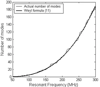
mean number of modes of the regular cavity, whose eigenfrequencies have well known analytical expressions. This result is easily illustrated in Fig. 1, where both the actual cumulative number of modes N(f), found analytically, and
Navg, obtained from (10) are plotted versus the frequency, for
the first 200 modes.
Fig. 1. Cumulative number of modes for cavity_1.
Equation (10) is more than an approximation: it gives the mean value of the number of modes.
B. Eigenvalue Spacing Distribution
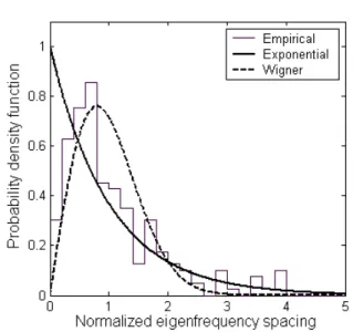
As explained in Section II-F, the eigenvalue spacing distribution can be used to check if a system is chaotic or not. The resonant frequency spacing is unfolded following the procedure described in Section II-F, leading to a normalized s spacing. As TE/TM degeneracies occur, s is calculated from the sorted eigenfrequencies without degeneracy [6]. Figure 2 gives the probability density function (pdf) of exponential, Wigner and s empirical distributions.
Fig. 2. Probability density function of the eigenfrequency spacings s for cavity_1 and the theoretical exponential and Wigner pdfs, issued from (7) and (8).
Figure 2 shows clearly that the empirical data do not follow a Wigner distribution, characteristic of chaotic systems. Instead of binning the data to obtain the histogram of frequencies, we prefer to compare in the empirical cumulative density functions (cdf) to the theoretical cdfs, as shown in Fig. 3.
Fig. 3. Cdf of s parameter, integrable cavity_1.
Figure 3 indicates that the s parameter follows an exponential distribution, as expected for this regular system. This point is confirmed by the low value ν = 0.07 of the Brody parameter estimated by curve fitting.
A last fact must be brought to light: although no antenna is modelled in our modal approach, the mere insertion of a wire into the cavity for excitation purpose transforms the integrable system into a pseudointegrable one. This phenomenon has been studied theoretically and experimentally in [5] and [23].
IV. REGULAR CAVITY WITH STIRRER_1
The RC_1 contains a metallic stirrer, which is a 2D rectangular plate parallel to the cavity bottom and which rotates around a vertical axis placed at the stirrer center at the height h = 2.2 m. The stirrer dimensions in meters are (la, lb) =
(1.5, 0.75). The stirrer orientation used in this Section (28° between the larger stirrer dimension and Ox axis) is sketched in Fig. 4.
Fig. 4. RC_1 with stirrer_1 into the integrable cavity_1.
Figure 4 also represents the 140 points (*) at which the field is calculated (cf. Section IV-D).
A. Mode Determination
Using FEM, the discretization of the electromagnetic problem leads to a generalized eigenproblem that is solved using Jacobi-Davidson algorithm [9]. We are looking for the first N = 200 modes: the subspace dimension is taken to be 2N, and the amount of memory required for such task does not permit to solve a very large eigenproblem. In order to reduce the number of DoFs, first order shape elements (instead of second order) are used to model the field on the unstructured mesh which is hand made reffined on the stirrer. This results in 60 103 DoFs for the stirrer position indicated in Fig. 4, and the run time is 4.5 103 s (Pentium IV, 3.2 GHz). It must be pointed out that the solver determines all the modes, even if they degenerate. Thus there is no risk of missing some modes, as happens in experimental procedures using the spectrum peaks. This is an important issue when the cumulative number of modes is estimated [6].
Another important issue is the existence of a systematic error in the eigenfrequency determination, due to FEM discretization. This is particularly true for the higher rank modes.
As a result we notice that the stirrer presence suppresses mode degeneracy: for instance, the perturbation by the stirrer of the TE111 and TM111 modes (resonant frequency 91.6 MHz)
leads to two distinct resonance frequencies (90.2 and 92.3 MHz). This important fact means that RC designers do not need to choose cavity dimensions such that degeneracy is avoided. For instance, it has been experimentally and numerically shown by Bruns and Vahldieck in [24] that cubic cavities can yield the same field uniformity as rectangular
cavities.
B. Weyl Formula
As the stirrer modifies the RC geometry, the mean number of modes must be evaluated using equations (3-4). The dihedral
angle is still
( )
2
π
ϕ
r
r
=
, but the contribution of Stirrer_1 leads toκ
=
L
x+
L
y+
L
z−
(
l
a+
l
b)
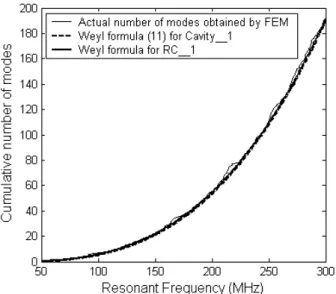
. The cumulative number of modes of RC_1 is determined numerically by FEM calculations, and is theoretically predicted by the Weyl formula. The result is plotted in Fig. 5 and can be compared to the case of cavity_1.Fig. 5. Cumulative number of modes for RC_1 obtained by FEM and the Weyl formula.
Figure 5 proves that the insertion of the stirrer in Cavity_1 leads to a negligible increase of the mode number. The slight difference between the Weyl formula and the averaged curve deduced from mode counting can be attributed to discretization errors inherent to the FEM: this makes impossible a precise determination of the resonant frequencies. In order to estimate the fluctuations of the density of modes, a polynomial curve fitting of order 3 is used to determine Navg(f).
C. Eigenvalue Spacing Distribution
From the first 200 eigenvalues of RC_1 and the numerical expression of Navg, the normalized spacings s are calculated
then classed into bins of width 0.2. The empirical pdf and the theoretical predictions are given in Fig. 6.
Fig. 6. Probability density function of the eigenfrequency spacings s for RC_1 and the theoretical exponential and Wigner pdfs.
A slight level repulsion, predicted in §IIF for chaotic systems, can be observed in Fig. 6, as confirm the cdfs plotted in Fig. 7.
Fig. 7. Cdf of s parameter, stirrer_1 into the integrable cavity_1.
In spite of a little discrepancy for small s values, the general behavior deduced from the first 200 modes of RC_1 is characteristic of an integrable system. The Brody parameter is ν = 0.15.
D. Eigenfields
The solver of the modal FEM problem provides the eigenfrequencies and the eigenfields inside the RC. These fields are projected onto a grid whose steps in the x, y and z directions are respectively Lx/10, Ly/10 and Lz/10, thus roughly 0.2 m. The x, y, and z components of the electric field are then collected; we only retained the values corresponding to points distanced from the walls by at least 0.5 m, as indicated in Fig. 4. In order to process uncorrelated data, we adopt 100 as the minimum mode rank, or f = 242 MHz: this way, the spatial step is larger than λ/4.
Figure 8 shows two kinds of histogram occurring for the Ex
component.
Fig. 8. Histograms of Ex values for the mode rank 106 and 190, RC_1.
The Ex component of mode #106 does not seem to follow a
Gaussian distribution, unlike mode #190.
In order to quantify the goodness-of-fit (GoF) of the empiric data to a Gaussian distribution with unknown parameters, the Shapiro-Wilks test is used. The result of this test is 0 if the hypothesis (data follow a normal distribution) is retained and 1 if rejected. The result of the GoF for the Ex component is
shown in Fig. 9, at a 0.05 significance level.
Fig. 9. Result of Shapiro-Wilks normality test for the Ex component, RC_1. Result is 0 when the data follow a normal law, at 0.05 significance level.
Figure 9 proves that Ex is not normally distributed for many
modes of RC_1. To get a global idea, the mean values of GoF tests for the mode ranks between 100 and 200 (i.e. 242 and 304 MHz) are respectively 0.22, 0.29, and 0.44 for the components Ex, Ey and Ez6. This discrepancy can be explained
by the poorly chaotic behavior of RC_1.
V. NON REGULAR CAVITY_2WITH STIRRER_2 A cavity corner is replaced by one eighth of a spherical surface of radius r, transforming the integrable cavity_1 into a nonintegrable cavity_2 of Sinai type. This technique is derived from the work of Dorr [7]. A V-folded Stirrer_2 with centered vertical rotating axis is oriented by 28° angle as shown in Fig. 10.
6
The difference between the 3 components is due to the shape of RC_1 where x and y play a rather similar role.
Fig. 10. Modeled RC_2 with stirrer_2 into the nonintegrable cavity_2. The 140 points at which the field is evaluated are indicated by (*).
A. Weyl Formula
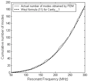
As explained by Arnaut in [18], the corner modifies the cavity geometry but (3-4) can still be used. Despite the small reduction of the cavity volume, the negative κ parameter is increased, resulting from the increase of the edge length and the curved surface. The overall consequence is that the mode density for cavity_2 can be larger than for cavity_1. Because of the complex geometry of the stirrer_2, we will not try to predict the accurate Weyl formula for RC_2, but we consider (11), obtained for cavity_1, as a good approximation of the cumulative number of modes for RC_2. To check this point, we compare in Fig. 12 the number of modes (10) of the cavity_1 to the one determined after FEM solving for RC_2.
Fig. 11. Cumulative number of modes for RC_2 obtained by FEM and Weyl formula for Cavity_1.
As seen in Fig. 11, Eq. (10) provides a good approximation of the number of modes of RC_2 even if it does not strictly apply to this enclosure. This satisfactory concordance justifies the use by practitioners of (10) or (5).
B. Eigenvalue Spacing Distribution
Navg(f) is obtained by a third order curve fitting of Fig. 11.
Then the variate s is calculated using (6) and the pdf of s is plotted in Fig. 12.
Fig. 12. Probability density function of the eigenfrequency spacings s for RC_2 and the theoretical exponential and Wigner pdfs.
The level repulsion at s = 0 can be clearly seen in Figure 12 for empirical data.
Fig. 13. Cdf of s parameter, stirrer_2 into nonintegrable Cavity_2.
A clear difference exists between Fig. 13 and Figs. 3 and 7. The Brody parameter is ν = 0.61. The Wigner distribution acceptably7 fits the empirical data issued from solely 200 eigenfrequencies. Small spacings are less probable (level repulsion) and large spacings are also improbable, as the maximum value is sMax = 3.16.
This tends to prove that the level fluctuation laws, derived from RMT, are also valid for the vectorial solution of the Helmholtz equation. Finally, the RC chaoticity is easily
7
A better result is reported in [6], where the cavity shape is very irregular, and the number of modes is higher (466).
assessed from a relatively small set of eigenvalues, as indicates Table I.
TABLE I
BRODY PARAMETER FOR DIFFERENT RC GEOMETRY.
Cavity_1 RC_1 RC_2
0.07 0.16 0.61
It is worth noting that despite the complex geometry of RC_2, the frequency spacing does not follow exactly the Wigner distribution. This is consistent with the fact that RMT is supposed to strictly apply in the limit λ/L <<1, where L is a geometric dimension.
C. Eigenfields
The result of the GoF for the Ex component is shown in Fig.
14.
Fig. 14. Result of Shapiro-Wilks normality test for the Ex component, RC_2. Result is 0 when the data follow a normal law, at 0.05 significance level.
Comparing Fig. 14 to Fig. 9, one can see that the Gaussian hypothesis is reasonable for more modes with RC_2 than with RC_1. For instance, the mean values of the GoF tests for ranks between 100 and 200 (i.e. 242 and 304 MHz) are respectively 0.14, 0.23 and 0.19 for the Ex, Ey and Ez component8. Moreoever, the small9 values show that most of the modes close to the Lowest Useable Frequency10 (LUF) correspond to a Gaussian distribution.
Nevertheless, the strict interpretation of Figs 13 and 14 leads to the following conclusion: as the eigenfield distribution is not perfectly Gaussian, RC_2 presents a non universal behavior at low frequencies. This means that the geometry details, such as the shape of the stirrer, play a crucial role to obtain the desired uniformity and isotropy of the field. Because of this non universality, the performance of two RCs can be compared: it is usually done by a uniformity test on the overall field, but could also be deduced from comparisons of the distributions of the eigenfrequency spacings or of the
8 The isotropy of the modes is better for RC_2 rather for RC1: RC_2has no particular symmetry.
9 If the data are normally distributed, as for high rank modes, the GoF test with 5% significance level rejects the Gaussian hypothesis with a probability of 0.05.
10
Here we use the common estimation that gives LUF = 3 fmin = 206 MHz.. This is close to the 60th mode criterion, as shows Fig. 11.
eigenfield. In this case, ensemble statistics should be used for various RC realizations associated to independent stirrer positions.
VI. FREQUENCY PERTURBATION IN A CHAOTIC RC
A. Presentation
In the previous sections, two different RCs (regular cavity and simple stirrer, non regular cavity and more sophisticated stirrer) were analyzed at a given stirrer position.
In this section the effect of the stirrer rotation on the resonant frequencies is investigated, following the work of Wu and Chang [25] who modelled a 2-D RC by TLM. Employing this technique, the resonant frequencies are determined indirectly: they are the maxima of the frequency response obtained by Fourier transform of an impulse time response. The implicit time windowing makes it difficult to separate close modes, and the determination of the frequency sweeps is uneasy.
With a modal approach, the eigenfrequency perturbations (or evolutions with the stirrer position) are determined directly and can be characterized more precisely. We will first check in this section that the modal density is not affected by the stirrer displacement. Then an illustration will be given of an important property: for a chaotic system, each eigenvalue curve proceeds without crossing any other. This general property does not come from RMT, and it can apply to a restricted number of modes.
In order to minimize the numerical noise due to FEM, the RC is discretized by second order elements, yielding 2 105 DoF. It takes 1500 s to find the first 20 modes. This determination is iterated for K stirrer positions evenly spaced by a 2° angle. For Stirrer_1, K = 90 using symmetry, and K = 180 for Stirrer_2.
B. Avoided Crossings
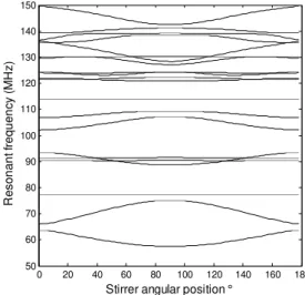
The values of the first 20 eigenfrequencies of RC_1 are plotted in Fig. 15. 0 20 40 60 80 100 120 140 160 180 50 60 70 80 90 100 110 120 130 140 150
Stirrer angular position °
R e s o n a n t fr e q u e n c y ( M H z )
Fig. 15. First resonant frequencies of RC_1 versus the stirrer displacement.
Figure 15 shows that the stirrer rotation does not increase the number of modes and produces frequency sweeps. Due to the special configuration of Stirrer_1, some modes are
unperturbed, such as the third one that is similar to TM110 of
the cavity_1.
As RC_1 does not present a chaotic behavior, crossings situations can be observed: a detail of Fig. 15 is given in Fig. 16, concerning the modes of ranks 4~6 and 14~17 at the first stirrer position. 0 100 200 125 130 135 140
Without Mode Tracking
0 100 200 125
130 135 140
With Mode Tracking
0 100 200 88 90 92 94 R e s o n a n t fr e q u e n c y ( M H z ) 0 100 200 88 90 92 94
Stirrer angular position °
Fig. 16. Details of Fig. 15 for the rank sorted eigenfrequencies (without tracking), and evolution of each of these modes after using the Mode Tracking Procedure [11].
The resonant frequencies being sorted by the solver, a given frequency rank is not related to a same mode when crossing situations occur: this is the case of the mode starting at 93.7 MHz. To detect automatically the crossings and assign the correct rank to a given mode, a mode tracking procedure (MTP) has been designed [11]. For the sake of completeness, the method is briefly presented in the Appendix. Applying the MTP, each frequency rank is related to a single mode, as shows Fig. 16.
In order to illustrate the level repulsion related to avoided crossings for RC_2, Fig. 17 plots the evolutions of the sorted eigenfrequencies. 0 50 100 150 200 250 300 350 50 60 70 80 90 100 110 120 130 140 150 Angular position ° R e s o n a n t fr e q u e n c y ( M H z )
Fig. 17. First resonant frequencies of RC_2 versus the stirrer displacement
For many modes (e.g. ranks 2, 3 and 7, 8, 9), the curves get close but no apparent crossing occurs. This fact has been confirmed by the MTP for the first 20 modes: the rank of each mode is the same during the stirrer rotation.
Finally, we can retain that a chaotic system presents avoided crossings. Therefore, the eigenfrequency perturbation induced by the stirrer is bounded by the mean spacing between nearest neighbor eigenfrequencies. As this one is proportionnal to the inverse of the modal density (3) that increases with the frequency, the eigenvalues perturbation tends to vanish at high frequencies. Since the resulting field is expanded on the same set of modes, it is most likely that the eigenfield perturbation plays a key role in the stirring process at high frequency. This phenomenon has been discussed in [11] for low frequencies.
VII. CONCLUSION
This paper presents a study of the chaos in a Reverberation Chamber (RC) derived from the analyze of its modal distributions and making use of quantum chaos theory. This theory is often validated by electromagnetic experiments, usually with empty 3-D cavities. We have extended the application to RCs, cavities containing a stirrer.
The Weyl formula is checked from the FEM determination of the first 200 modes of RCs with different shapes from integrable to chaotic.
The distribution function of the eigenfrequency spacing is in agreement with Random Matrix Theory (RMT) and reveals the RC chaoticity. The eigenmode distributions are also analyzed and compared to the theoretical Gaussian distribution: close to the lower useable frequency, the modes of the studied chaotic RC fairly respect this asymptotic property.
Although RMT assumes that a great number of modes (and consequently high frequency modes) must be analyzed, we have seen that our restricted number of modes allows an illustration of the universal properties of the RC, i.e. properties that are independent from the exact RC shape. However, some non universal behaviors have also been noticed. These deviations from the theoretical limit can be used as a metric to compare RC performances.
Using a Mode Tracking Procedure, we have illustrated the following property of a chaotic RC: during a stirrer displacement, the curves of the resonant frequencies do not cross. This means that at high frequency the frequency sweeps tend to vanish.
VIII. APPENDIX
The key to the mode tracking procedure [13] is sketched here to make this paper self-explanatory.
At stirrer position k (1 ≤ k ≤ K), the solver provides a set of
N eigenvalues
f
n(k
)
and eigenvectorsE
n(k
)
r
. The objective is to track the modes from the first stirrer position till the position k. For this, we first look for an index permutation vector that models correctly the transition between the stirrer positions k and k+1.
are orthogonal: for the stirrer position k, two different eigenvectors
E
m(k
)
r
and
E
n(k
)
r
verify (15), where Ω is the cavity domain :
(
Em(k),En(k))
=0=∫∫∫
ΩEm(k).En (k)dV r r r r (11) The idea is that (15) is quite respected for a small rotation step, considering two eigenvectors corresponding to adjacent positions, sayE
m(k
)
r
and
E
n(
k
+
1
)
r
. Discretizing the fields
)
(k
E
mr
on a uniform grid yields
U
m(k
)
r
vectors, (11) can be generalized as (12)( )
m,n =U (k)U (k+1) Sk mT n r r , (12)where T designs the transpose. After normalizing
U
m(k
)
r
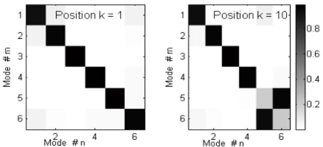
, Sk matrix is numerically close to a permutation matrix, thus enabling a crossing detection. For example, a Sk view is given in Fig. 18 for the first 6 modes of RC_1.
Fig. 18. Abs(Sk) matrices for k = 1 and k = 10, first 6 modes of RC_1.
Sk=1 can be assimilated to identity (no crossing) whereas Sk=10
is a permutation matrix affecting the ranks 5 and 6 (mode 6 at position 10 will occupy the rank 5 at position 11).
The permutation vectors are easy to identify in most of the cases, but not all, as indicates the S23 matrix (Fig. 19).
Fig. 19. Abs(S23) matrix, first 6 modes of RC_1.
According to S23 values, the transition between k = 23 and k = 24 is uncertain. As tracking the modes from the first position till the position k is an iterative procedure, it can be dramatically affected by error propagation. To get a robust technique, we consider multiple possibilities (e.g. 2 choices at position k = 23). Then a tree is constructed for the solutions
ensemble. The selection of the best (or actual) solution is based on the regularity of the eigenvector projection on the initial eigenvector (more details in [11]).
REFERENCES
[1] D. A. Hill, “Plane wave integral representation for fields in reverberation chambers,” IEEE Trans. Electromag. Compat., vol. 40, no. 3, pp. 209-217, Aug. 1998.
[2] L. Cappetta, M. Feo, V. Fiumara, V. Pierro, and I. Pinto, “Electromagnetic chaos in mode-stirred reverberation enclosures”, IEEE Trans. Electromag. Compat., vol. 40, no. 3, pp. 185-192, Aug. 1998.
[3] H. J. Stöckmann and J. Stein, “Quantum chaos in billiards studied by microwave absorption”, Phys. Rev. Letters, vol. 64, no. 19, pp. 2215-2218, May 1990.
[4] S. Sridhar, “Experimental observation of scarred eigenfunctions of chaotic microwaves cavities”, Phys. Rev. Letters, vol. 67, no. 7, pp. 785-788, Aug. 1991.
[5] F. Haake et al., “Manifestation of wave chaos in pseudointegrable microwave resonators”, Phys. Rev. A, vol. 44, no. 10, pp. 6161-6163, Nov. 1991.
[6] S. Deus, P. M. Koch, and L. Sirko, “Statistical properties of the eigenfrequency distribution of the three-dimensional microwave cavities,” Phys. Rev. E, vol. 52, no. 1, pp. 1146-1155, Jul. 1995. [7] U. Dörr, H. J. Stöckmann, M. Barth, and U. Kuhl, “Scarred and
chaotic field distributions in a three-dimensional Sinai-microwave resonator,” Phys. Rev. Letters, vol. 80, no. 5, pp. 1030-1033, Feb. 1998.
[8] C. F. Bunting, K. J. Moeller, C. J. Reddy, and S. A. Scearce, “A two-dimensional finite-element analysis of reverberation chambers”, IEEE Trans. Electromag. Compat., vol. 41, pp. 280-289, Nov. 1999.
[9] G. Orjubin, E. Richalot, S. Mengué, M-F. Wong, and O. Picon, “On the FEM modal approach for a reverberation chamber analysing”, IEEE Trans. Electromag. Compat., vol. 48, pp. -, Fev. 2007.
[10] H.-J. Stöckmann, Quantum Chaos. An Introduction, Cambridge Univerity Press, Cambridge, 1999.
[11] G. Orjubin, E. Richalot, S. Mengué, and O. Picon, “Mode Perturbation Induced by the Stirrer Rotation in a Reverberating Chamber”, in Proc. of EMC Zurich 2005, pp. 39-42, Zurich, Feb. 2005.
[12] J. Barthémely, O. Legrand, and F. Mortessagne, “Complete S matrix in a microwave cavity at room temperature”, Phys. Rev. E, vol. 71, pp. 016205-1-016205-11, 2005.
[13] V. Galdi, I. M. Pinto, and L. B. Felsen, “Wave propagation in ray-chaotic enclosures: Paradigms, oddities and examples, IEEE Antennas and Propagation Magazine, Vol. 47, No. 1, pp. 62-81, Feb. 2005.
[14] M.V. Berry, “Regular and irregular semiclassical wavefunctions’” J. Phys. A, vol. 10, no. 12, pp. 2083-2091, 1977.
[15] A. Kudrolli, V. Kidambi, and S. Sridhar, “Experimental studies of chaos and localization in quantum wave billiards”, Phys. Rev. Lett., vol. 75, no. 5, pp. 822-825, Jul. 1995.
[16] L. R. Arnaut and P. D. West, “Evaluation of the NPL untuned stadium reverberation chamber using mechanical and electronic stirring techniques”, NPL Report CEM 11, National Physical Laboratory, United Kingdom, Aug. 1998.
[17] R. Balian and C. Bloch, “Distribution of eigenfrequencies for the wave equation in a finite domain: III. Eigenfrequency density oscillations,” Ann. Phys. (NY), vol. 69, pp. 76-160, 1972.
[18] L. R. Arnaut, “Operation of electromagnetic reverberation chambers with wave diffractors at relatively low frequencies”, IEEE Trans. Electromagn. Compat., pp. 637-653, Nov. 2001. [19] M. V. Berry, “Semiclassical theory of spectral rigidity,” Proc. R.
Soc. Lond. A, vol. 400, pp. 229-251, 1985.
[20] L. K. Warne et al., “Statistical properties of a linear antenna impedance in an electrically large cavity,” IEEE Trans. Antennas and Propag., vol. 51, no. 5, pp. 978-992, May 2003. [21] H. P. Baltes, ”Asymptotic eigenvalue distribution for the wave
equation in a cylinder of arbitrary cross section,” Phys. Rev. A, vol. 6, no. 6, pp. 2252-2257, 1972.
[22] B. H. Liu, D. C. Chang, and M. T. Ma, Eigenmodes and the composite quality factor of a reverberating chamber, Nat. Bur. Stand. (U.S.) Tech. Note 1066, 1983.
[23] D. Laurent, O. Legrand, and F. Mortessagne, “Diffractive orbits in the length spectrum of a two-dimensional microwave cavity with a small scatter” Phys. Rev. E, vol. 74, no. 4, pp. -, . 2006. [24] C. Bruns and R. Vahldieck, “A closer look at reverberation
chambers—3-D simulation and experimental verification,” IEEE Trans. Electromag. Compat., vol. 47, no. 3, pp. 612-626, Aug. 2005.
[25] D. I. Wu and D. C. Chang, “The effect of an electrically large stirrer in a mode-stirred chamber”, IEEE Trans. Electromag. Compat., vol. 31, pp. 164-169, May 1989.