From observed successions to quantified time: formalizing the basic steps of chronological reasoning

HAL Id: hal-02326183

https://hal-paris1.archives-ouvertes.fr/hal-02326183

HAL is a multi-disciplinary open access archive for the deposit and dissemination of sci-entific research documents, whether they are pub-lished or not. The documents may come from teaching and research institutions in France or abroad, or from public or private research centers.

L’archive ouverte pluridisciplinaire HAL, est destinée au dépôt et à la diffusion de documents scientifiques de niveau recherche, publiés ou non, émanant des établissements d’enseignement et de recherche français ou étrangers, des laboratoires publics ou privés.

From observed successions to quantified time:

formalizing the basic steps of chronological reasoning

Bruno Desachy

To cite this version:

Bruno Desachy. From observed successions to quantified time: formalizing the basic steps of chrono-logical reasoning. ACTA IMEKO, International Measurement Confederation (IMEKO), 2016, 5 (2), pp.4. �10.21014/acta_imeko.v5i2.353�. �hal-02326183�

ACTA IMEKO 

From observed successions to quantified time: formalizing 

the basic steps of chronological reasoning 

Bruno Desachy 

Since the concepts rethinking carried out by E.C. Harris in the 1970s about archaeological stratigraphy [1], [2], the stratigraphic observations have become more rigorously recorded and processed. On the other hand, it is well known that the possibilities to get “absolute” (more exactly: quantified) indications of time about archaeological remains have been in constant progress for the past sixty years, thanks to the laboratory dating techniques.

However, these advances in relative and “absolute” chronology still leave some dark zones in the basic chronological reasoning used in field archaeology. As some authors said [3]-[5], usual archaeological discourses are widely implicit and sometimes ambiguous about dating (i.e. positioning in the quantified time) the observed stratigraphic units and the historical material entities that archaeologists deduce from these units. This paper, derived from a work in progress about formalisation of stratigraphic data processing and chronological reasoning in field archaeology [6]-[9], presents some elements specifically devoted to this moving from the stratigraphic relative chronology analysed from field observations to a

quantified frame of time using different dating sources.

After reminding some notions of formalization of stratigraphic relative chronology – which is the basis of the chronological reasoning discussed here – in Section 2, we will expose the proposed framework and process to integrate the observed relative chronology in a quantified time frame, taking in account the variety of available dating (Section 3). The next two sections are about grouping, used to get a more global chronological view (Section 4), and about the double nature of time in the chronological reasoning used by field archaeologists: stratigraphic time related to the formation of ground units and historical time related to the material entities use life (Section 5). Section 6 returns to one important issue: the uncertainties tied to the dating. In the last section, computerized tools derived from this work are briefly presented (Section 7).

2. REMINDERS ABOUT FORMALISATION OF RELATIVE  STRATIGRAPHIC TIME 

2.1. Harris matrix 

The stratigraphic analysis proposed by Harris [1] is based on the systematic recording and processing of chronological order ABSTRACT 

This paper is about the chronological reasoning used by field archaeologists. It presents a formalized and computerizable but simple  way  to  make  more  rigorous  and  explicit  the  moving  from  the  stratigraphic  relative  chronology  to  the  quantified  “absolute”  time,  adding to the usual Terminus Post Quem and Terminus Ante Quem notions an extended system of inaccuracy intervals which limits the  beginnings, ends and durations of stratigraphic units and relationships. These intervals may be processed as an inequations system,  integrating  stratigraphic  order  relationships  and  available  dating  sources.  Questions  about  chronological  units  grouping,  about  the  differences between stratigraphic time and historical time, about the extension of the exposed chronological frame to historic entities,  and  about  the  processing  of  uncertainties,  are  discussed.  Finally,  the  present  state  of  computerized  tools  using  this  way  is  briefly  indicated. 

relationships deduced from observed interfaces between archaeological (and natural) layers. It involves a precise definition of the stratigraphic unit as a discrete unit of time identified by these interfaces, and also characterized by a spatial location, and a functional, social or cultural interpretation corresponding to the human or natural action behind the formation of the unit.

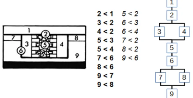
The stratigraphic analysis process is summarized by a well-known Harris' example (Figure 1): in the field, interfaces are observed and recorded, resulting in a set of units and order relationships. This set may be simplified by removing the “redundant” relationships (i.e. transitively deductible relationships) following the Harris' so called “fourth law of archaeological stratigraphy”. A graph (“Harris matrix”) displays this simplified (but complete) relative chronology.

2.2. Mathematical and computerized approaches 

The analytical concepts proposed by Harris and the logical framework behind the making of a Harris Matrix made possible mathematical formalizations. Different searchers have worked on such formalizations, from the earliest characterizations of the Harris Matrix as a partially ordered set [10], to recent works integrating formalized processing of stratigraphic sequences with GIS and spatial analyses [11], [12]. These works resulted in some computerized tools, able to draw automatically a Harris Matrix, for instance Stratify [13], MatrixComposer [14], or our application Le Stratifiant [6]. These proposals have in common to consider observed stratigraphic relationships as order relationships with their properties of reflexivity, asymmetry (or antisymmetry) and transitivity, and to use applications of graph theory to process these relationships. In particular, the Harris Matrix is formally close to task scheduling graphs developed in the 1950s to manage complex production processes [15], [16].

Beyond this common basis, the way we chose to process stratigraphic data [6]-[9], has some peculiarities. The first is an algorithm (derived from the MPM graph method [17]) using an adjacency matrix to calculate a critical path value (i.e. irreducible relative time distance) for each couple of units and a stratigraphic rank for each unit; these values and ranks allow to provide a graph corresponding to a Harris Matrix. A second peculiarity is the display of the graph, chosen to avoid broken lines (which may become visually quite complex and ambiguous in big graphs) and using only vertical lines to order relationships and horizontal links to synchronisms [7] (Figure 2).

2.3. The choice of admitting uncertain stratigraphic relationships  The most important peculiarity of our approach, materialized in the application Le stratifiant, is the possibility of

processing uncertain relationships.

Indeed, some doubts may appear in the field observations. It is the case with the notion of “correlation”, derived from Geology, and used by Harris to record a synchronic relationship between two layers, considered as the same stratigraphic step. Formally, a stratigraphic synchronism is a mathematical equivalence relation with its properties of reflexivity, symmetry and transitivity. If the synchronism is certain, the order relationships of the synchronic units may be merged, and there is no need to display on the graph the order relationships deductible by this synchronism.

But as S. Roskams noticed [18], a stratigraphic “correlation” may be extrapolated rather than observed. For instance, in the original example retaken Figure 1, Harris assumed that the units 7 and 8 may originally be a same floor, so they are correlated. But they were cut by the trench 6 so that the original continuity can no more be observed; thus this synchronism is only a guess. Even if this assumption is based on significant indications, it is less certain than an observed continuity.

To take in account this lower level of certainty, practically used by field archaeologists when they assume (and not observe) a synchronism, we have developed a simple way, derived from modal logic: an “uncertain” (or “estimated”) logical modality can be recorded for a synchronism. In this case, a same stratigraphic rank is calculated for the “perhaps” synchronic units but their order relationships are not merged (Figure 3).

These two levels of certainty – certain and “estimate” (uncertain) – are logically applicable also to the order stratigraphic relationships. Practically, they correspond to some

Figure 2. Matrix processing to generate a stratigraphic graph [7]: observed  relationships  (corresponding  to  Figure  1)  are  recorded  on  an  adjacency matrix; then the matrix is processed to calculate critical path values for each  couple, providing a stratigraphic rank for each unit. The processed matrix is then scanned to draw the graph, using stratigraphic ranks to place the units  and displaying only the non‐deductible relationships (value: one). 

Figure 1. Left: simplified example of stratification (slightly modified from [2]  p.87  Fig.28);  2  (horizontal  cut)  and  6  (foundation  trench)  are  not  deposits but erosion units. Middle: observed order relationships; italics: "redundant" (deductible) relationships, not displayed on the graph. Right: Harris matrix. 

Figure 3. From the example Figure 1, stratigraphic  graph  in case of certain  synchronism  between  units  7  and  8  (left),  or  in  case  of  uncertain  synchronism (right).  

cases of difficult or limited conditions of observation, so that the archaeologist can make assumptions but he has too few indications to record a certain relationship (for instance during a standing building study, if the archaeologist is not allowed to destroy the building to confirm a relationship…). Indeed, as M. Carver [19] said: “stratification is not always obvious and our readings of it are often uncertain”. In every case, distinguishing between certain and uncertain is the responsibility of the field archaeologist, who must not exceed his limits of skill [9].

Then, the rule of elimination of deductible relationships (on the graph) is applied only within the same level of certainty: if a certain order relationship is “redundant” compared to an uncertain one, it is not eliminated, in order to display the continuity of the certain relative chronology (Figure 4).

During the processing, possible contradictions between relationships provided with their certainty / uncertainty modalities result in logical cases of confirmation, invalidation (of an uncertain relation by certain ones), contradictory uncertainty (between uncertain relationships), or contradiction (between certain relationships). The two last cases need a user intervention to correct (or eliminate) the wrong data.

3. QUANTIFIED STRATIGRAPHIC TIME 

3.1. Dating relative time: the usual TPQ‐TAQ way 

After identifying, recording and processing the stratigraphic relative chronology, the second step of the chronological reasoning is to place this succession in a quantified time frame.

As said in the introduction, the great progresses of the laboratory dating techniques are well known. However, the quantified time indications from these laboratory techniques (as well as those provided by more classical – historical, numismatic, etc. – chronometric sources), are not direct solutions to the problem of relative chronological units dating; they are only parameters of this problem.

A lot of literature has been written about using contextual (thus stratigraphic) data to date archaeological objects, since the 19th _{century and the cross-dating method. The reverse way –}

dating a stratigraphic unit from different possible quantified time indications, which is our subject here – is curiously less explored, and usually limited to the TPQ use. Indeed, the most common way to apply dating indications to a stratigraphic unit is the Terminus Post Quem (TPQ) notion [3]. A TPQ is a “not before” date: an earlier endpoint for the unit chronological position. Usually, the TPQ of a unit is provided by the most recent dated object found in this unit.

A complementary notion –Terminus Ante Quem (TAQ) or “not after” date – refers to the later endpoint for the unit chronological position. It is usually provided by an extrinsic source concerning the unit, for instance historical documentation. The couple TPQ-TAQ forms an inaccuracy interval, bounding a precise (and generally unknown) date

assignable to the stratigraphic unit.

Well-known rules are applicable to transfer these endpoints by the way of stratigraphic relationships: a TPQ may be applied to each subsequent unit (if it has no later TPQ), and a TAQ may be applied to each prior unit (if it has no earlier TAQ). These rules are the traditional way to integrate stratigraphic constraints into the dating of objects or structures. They were taken in account by some computerized dating formalizations (for instance [20], [21]), and the TPQ endpoint is de facto used in the probabilistic models integrating stratigraphic constraints in laboratory dating techniques, like Chronomodel [22] or Oxcal.

However, the use of this [TPQ, TAQ] interval raises some issues. First, as noticed by several authors [3], [4] and as it still appears in many excavation reports, TPQ is sometimes confused with the real chronological position of the deposit, in statements like “the ditch filling contains a Roman sherd, so the ditch is Roman”; that is at least a dangerous shortcut, because a deposit may be much more recent than the object it contains. The TPQ using rules are well known, but sometimes we forget them, especially if it is convenient for our chronological hypothesis [4].

More fundamentally, there is an ambiguity about the position of the TPQ related to the deposit. It is recognized that the TPQ is a limit at the earliest for the position of the unit; but what limit exactly: the beginning or the end of the unit formation? Actually, the most recent object found in a given unit (usual definition of the TPQ, as said above) corresponds to the earliest date to its formation end, and not to its formation beginning (because an object made after the formation beginning of a unit may be deposited in this unit, if the formation duration is long enough). However, by another dangerous shortcut, the TPQ is often taken as an absolute “no before” date, relevant also to the beginning of the deposit formation. Another aspect of this ambiguity is the no accounting (or the rare accounting) for the duration of formation of the considered unit. The [TPQ, TAQ] interval limits a moment (the final moment) of the unit, not its duration. So, indications of formation duration, when they are available (geoarchaeological observations for instance) are not or bad taken in account in the whole chronological reasoning of dating. Finally, a reasoning only based on the [TPQ, TAQ] interval tends to reduce intellectually the unit temporality to a simple date – just a moment in time without duration – what is all the more untoward that the duration is actually long.

In other words, we think that the usual TPQ-TAQ notions are an incomplete frame for the stratigraphic units dating. 3.2. Taking durations in account: a system of inaccuracy intervals 

Our proposal consists in adapting the quantified frame of time used in the industrial applications of graph theory mentioned above [17]. This frame includes only four main variables. Three concern each single chronological unit i: the beginning Bi , the end Ei and the duration Di . A fourth variable

is necessary: the duration D_ij allocated to the order relationship (if it exists) between a unit i and a unit j (which may be zero if the succession is immediate). Theses variables are linked by basic equalities:

. (1)

For the order relationship i < j

. (2)

In a sequence i < j < k, the relationship i < k , transitively deductible, doesn't appear on the graph but it has a duration D_ik

so that:

. (3)

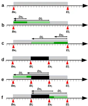
This simple frame is necessary but not sufficient to deal with archaeological data. As said above, the quantified time indications, with very few exceptions, do not directly provide values to these variables. They just can be used as limits of inaccuracy intervals including each basic variable (Figure 5). The limits of these inaccuracy intervals are Be (beginning at the earliest), Bl (beginning at the latest), Ee (end at the earliest), El (end at the latest), Ds (duration at the shortest), Dl (duration at the longest), so that, for a unit i:

, (4) , (5) . (6) And for an order relationship i < j:

. (7) We find again the [TPQ, TAQ] interval, which actually

corresponds to the [Ee, El] interval (cf. Section 3.1 below). Stratigraphic order relationships, basic equalities of quantified time (1), (2), (3) and their inaccuracy intervals (4), (5), (6), (7) may be integrated in a whole system of inequations, with its unknown values (basic variables Bi Ei Di Dij for each unit and

relationship) and its valued parameters (limits of inaccuracy intervals, provided by dating indication). If there is no indication for an endpoint, a default value is used. These default values must be previously defined to include the whole period concerned, between an “absolute beginning” (for instance: the Big Bang date, or perhaps a little later) used for the endpoints at the earliest, and an absolute end (for instance: now) used for the endpoints at the latest. The default value for the durations at the longest is the difference between the absolute end and the absolute beginning; the default value for the durations at the shortest is zero. In the examples below, the unit of quantified time is the year.

The main inequations are, for a unit i:

, solution of , (8)

, solution of , (9)

, solution of . (10)

And for an order relationship i < j

, solution of , (11)

, solution of ,(12)

, solution of .(13)

We can notice about the three last inequations that if we have no indications of duration (other than the default values), we find again the traditional rules of TPQ and TAQ transfer – cf. Section 3.1 above; but if we have some duration indications, we can improve the intervals of the related units.

For an order sequence i < j < k: , solution of

. (14)

The simple algebraic processing of this inequations system results in the best possible reduction of the inaccuracy intervals. 3.3. Impossible, possible, and certain time 

After processing, each unit has a slot of “possible time”, between the beginning at the earliest Be and the end at the latest El (Figure 6).

It is important to note that if we do not have enough accurate indications of beginning at the latest and end at the earliest (so that Bl > Ee), the existence of the unit will be uncertain at each moment in this “possible time”; because at any moment, the formation of the unit may be already finished or not yet started. The only certainty is negative: the formation of the unit is impossible before and after this “possible time”. It must not be confused with the unit duration: the duration at the longest is limited by the possible time, but may be shorter.

In favorable cases (if Bl < Ee: the latest date for the beginning of the unit is before the earliest date for the end), a slot of “certain time” exists, in whom it is certain that the unit was in the making. The certain time gives of course a minimal duration at the shortest. But a wider duration at the shortest may be known for the same unit. In this case, the position of this duration is partially known because it necessarily covers this

Figure  5.  Stratigraphic  ordered  time  (that  archaeologists  can  record  and process),  stratigraphic  quantified  time  (that  archaeologists  search)  and inaccuracy  intervals  in  quantified  time  (that  archaeologists  can  know  and process). 

Figure  6.  a‐c:  Possible  formation  time  of  a  unit  i  (a);  with  duration  indications: possible positions of i at the earliest (b) or at the latest (c); d‐f:  certain formation time for a unit i, if Bli < Eei (d); with duration indications:  possible positions of i at the earliest (e) and at the latest (f). 

certain time (Figure 6).

3.4. Example and graphic display 

Let us return to the example of Figure 1 and let us admit that a document – an old photography dated 1860 – shows the place without the wall corresponding to the unit 3. It means that this wall was already destroyed in 1860. This is a TAQ corresponding to the end at the latest of the destruction cut (unit 2). This limit (El2 = 1860) allows to reduce the possible

time for the unit 2; and thus for the stratigraphically previous units.

If we admit now that a coin minted in 1600 was found in the unit 3, this coin provides a TPQ for this unit i.e. a limit at the earliest only for its end (Ee3 = 1860). Consequently, a single Eei

value (with no other indications) does not allow reducing the “possible time” [Be_i, El_i]. In other words, contrary to what is often said, a TPQ does not precise the timeslot of the unit which contains it (because, as said above, it limits the end and not the beginning of this unit formation). However, it improves the “possible time” of the stratigraphically later units (here, units 2 and 1): if i < j, then of course Ee_i ≤ Be_j.

To precise the position of the unit 3, we need explicit duration indication. Let us admit that field observations indicate a short formation duration for the whole sequence formed by the units 3, 4, 5 and 6 (for instance because the foundation trench 6 is not collapsed, so it must have been filled quickly): certainly less than a year. So we have a Dl value for the unit 3. With these two known limits (Ee3 = 1600, Dl3= 1), we get a

beginning at the earliest (Be3 = 1600 – 1 = 1599) which reduces

the “possible time” for the unit 3 (cf. inequation (8) above). This duration estimate – necessary to get a beginning at the earliest from a TPQ provided by objects found in the units – is actually implicit and elided in many dating statements (the TPQ is then, as said above, improperly used to give directly an “absolute beginning” to the unit).

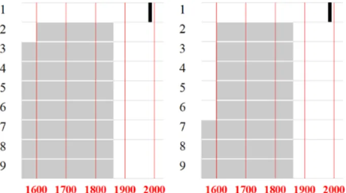
We get finally a [1599, 1860] “possible time” interval for the unit 3; and for the other units with a TPQ = 1860 and a no more than 1 year duration of formation.

We added to this example a case of “certain time” interval, admitting that the unit 1 is a contemporary floor of which the dates of beginning and end of construction are known with total certainty (1980, thus with a less than a year duration construction). In this case, the two endpoints of the inaccuracy interval have the same value (the inaccuracy range is zero). So there is no “possible time”, only a “certain time” for this unit 1.

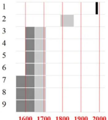
The result may be displayed by a graph on a quantitative timescale (Figure 7), complementary to the stratigraphic graph.

4. CHANGING TIMESCALE: SUBSET RELATION  

4.1. Grouping stratigraphic units 

Practically, the archaeologists have to deal with stratigraphic time at different scales.

After the analytic stage of identifying, recording and processing the stratigraphic units and relationships, the Harris matrix has also been designed to be a basis for the synthesis of the stratigraphic and chronological information [2].

Elementary units may be grouped in wider sets, providing a synthetic view of the site. This issue of grouping attracted much comment, and different ways exist. According to E. Harris [2], stratigraphic units can be grouped in chronological phases and periods. In a more functional way, M. Carver [19] suggests grouping the units in "features" (e.g. pit, ditch, grave, etc.) and "structures" (sets of features). A. Carandini [23] combines these two approaches in a system including grouping in functional "activities" and "groups of activities", and chronological phases and periods. This is also the case with the proposals from the centre national d'archéologie urbaine [24] including a double grouping scale in chronological sequences (i.e. elementary successions), phases, periods, and functional features and structures. The grouping process itself is formally seen by I. Sharon [25] as an "agglomerative model", after the "ordinal model" of stratigraphic units ordering. To A. Carandini [26], it reflects the progressive rise of the archaeological discourse, from basic observations until a historic level. Here, we consider this process from the point of view of its possible formalization and computerization. This point of view makes necessary an explicit distinction between two kinds of time: the stratigraphic temporality of the site formation process and the historic temporality linked to the evolution of the use of the site space (to which we will return in the Section 5 below).

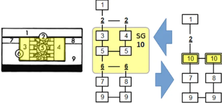
If the archaeologist considers the stratigraphic time of the formation of the material tracks, the grouping of the stratigraphic units may be simply formalized by a subset relation between a macro unit and its included units, allowing as many grouping levels as wished. Some computerized tools may display such subset relationships on the Harris matrix, as frames containing units, like Stratify [27]. We propose to use the adjacency matrix presented above (cf. Section 2.2) to formalize this subset relation processing (Figure 8). It allows to calculate the inclusion levels and to detect possible inconsistencies (unit including and included in the same other unit) (Figure 8).

We have chosen to make possible the transfer of the order

Figure 7. Harris' example: “possible time” (in grey) calculated only with TPQ‐ TAQ  intervals  (left),  and  with  duration  intervals  (right).  In  black:  “certain time” of the unit 1 (formation date accurately known). 

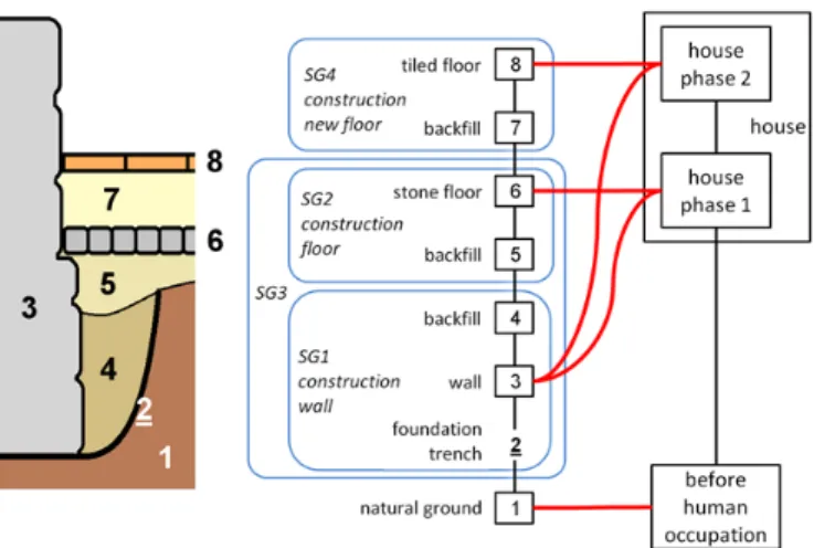
Figure 8. Example of stratigraphic grouping at two levels: the stratigraphic  group 1 (SG1) includes units related to the construction of the wall 3; SG2 includes  unit  related  to  the  construction  of  the  floor  6;  SG3  includes  the  whole sequence of construction. From the straightforward inclusions coded  on the adjacency matrix, the indirect inclusions and the inclusion levels may be calculated. 

relationships from elementary units to an upper level of grouping, so that, for the units i, j, k with i included in k:

, ⊂ , ⊄ ⇒ . (15)

In other terms, performing a stratigraphic grouping means that the order relationships between included and non-included units are merged and attributed to this grouping considered as a global unit. The internal order relationships (between units included in the grouping) are no more taken in account. This processing is similar to the synchronisms processing (cf. above); indeed, we can say that grouping a set of units is considering these units as synchronic, at a wider scale of time.

A reverse way is sometimes practised (especially in large excavations in “flat” rural sites without deep stratification): a whole stratigraphic feature may be first identified (for instance a ditch with its filling) and relationships with other features may be recorded at this level (for instance this whole ditch cuts another ditch), before a finer stratigraphic analysis (for instance a trench practised into this ditch, in order to observe its internal stratification, providing more detailed stratigraphic units and relationships). In this case, the reverse using of the same simple subset relation allows integrating these different recording levels in the most analytical possible chronology, at the included units level; so that, for the units i, j, k with i included in k:

, ⊂ ⇒ . (16)

In other words, included units inherit order relationships from their including unit (Figure 9).

4.2. Grouping in the stratigraphic quantified time 

To achieve stratigraphic groupings in the quantified time, inclusion relationships may be integrated in our inequations system.

From a first simple principle – the duration of an included unit is limited by the duration of the including unit – we can deduce the relations between the basic time variables of an including unit i and its included units j(i):

, (17)

. (18)

A second simple principle is, if order relationships exist between the included units, that the formation duration of the including unit can't be less than the critical path (minimum irreducible total duration) of the partially ordered set formed by the included units and relationships. So that, for an including unit i, its included units j(i) ⊂ i and k(i) ⊂ i and an order

relationship j(i) < k(i):

. (19)

From those basic inequalities result some inequalities linking the intervals limits of i and j(i) ⊂ i:

, (20)

, (21)

, (22)

. (23)

And for an including unit i, its included unit j(i) ⊂ i, k(i) ⊂ i and the order relationship j(i) < k(i):

, (24)

. (25)

From these inequalities and from the inequations exposed above (8 to 14), adapted inequations may be drawn to reduce the range of the inaccuracy intervals of the included and including units, following the internal and external order relationships of the including unit.

For instance, in the Harris example (Figure 1), we previously assumed that a set of units (3 to 6) has a whole duration at longest (1 year), which is an interval endpoint Dl recorded at a grouping level; then we have transferred this duration at longest from this grouping level to each elementary units (cf. above Section 3.4), which is a direct application of inequality (22); and we have grouped these units in a more synthetic unit (of construction) SG10 (Figure 9). In this simple example, the order relationship SG10 < 2 inherited from the included units provides a TAQ: ElSG10 = 1860. To find the possible time of

SG10, we can find its TPQ, using a simple inequation derived from the inequalities (20) to (23):

⊂ , . (26)

We have 3 ⊂ SG10, DlSG10 = 1 and Be3 = 1600, thus BeSG10 =

(1600-1) = 1599. In this way, this TPQ may be then directly transferred to the SG10 included units (under the inequality 20).

5. INFERRING HISTORICAL TIME FROM STRATIGRAPHIC  TIME 

5.1. Stratigraphic units and historical entities 

As said above, we have to deal with a double temporality: beyond the making of the stratigraphic chronology (including dating and grouping), there is another stage of chronological synthesis, which implies a change of nature of time.

The stratigraphic time, discussed until here, is strictly related to the formation of field units. For instance, in the Figures 1 and 9, the duration referred to the unit 3 (wall), as stratigraphic unit later than the unit 2 (foundation trench) and prior to the unit 4 (backfill), is only the formation duration of this unit 3 (i.e. the wall construction duration).

But if we want to approach the historical time of societies, we have to consider no more only the formation time of the material remains, but also their whole “cultural life”. In the same example, the historical time related to the wall corresponding to the unit 3 includes not only the construction duration, but also the period of use of this wall, as a part of an inhabited or used structure, until its destruction. This whole period of “cultural life” of a material remain, including use time, corresponds to the “systemic context” notion developed by M. Schiffer [28], opposed to the “archaeological context” of the

Figure 9. In the Harris example (cf. Figure 1 above), the set of units 3 to 6 may  be  grouped  in  a  macro  unit  of  construction  (stratigraphic  group  10). The graph may be displayed at the synthetic scale of the SG (which inherits relationships  from  its  included  units),  or  at  the  analytical  scale  of  the elementary  units  (which  inherit  relationships  possibly  recorded  at  the  SG level). 

buried remains which no more interact with an alive society. We can notice that this time in systemic context longer than the duration formation is a characteristic of units functionally interpretable as building or fitting out, by opposition to the “occupation” units whose formation duration corresponds to their whole time in systemic context (like material use tracks for instance). However, the stratigraphic time, limited to the formation durations of field units, does not take in account all the time in systemic context. This limit also applies to the Harris matrix, which displays only the stratigraphic time (that it is why some archaeologists like M. Carver [29], P. Paice [30] or J. Collis [31] have criticized it).

De facto, archaeologists deduce historical material entities (e.g. “structure”, “ditch”, “well” “house”, “temple”, “architectural ensemble”, etc.) from stratigraphic units, adding (explicitly or more often implicitly) use durations to formation durations, even if, as in the examples above, there are just construction units with no preserved material tracks (and so recordable as stratigraphic units) of their “occupation” (i.e. their use timespans). The functional groupings mentioned above (“feature”, “structures”…) correspond to such historical (and not only stratigraphic) entities, because they correspond to a more synchronic and historic (the life on the site at a given period) than diachronic and stratigraphic (the site formation process) view. It is also these historical entities, more than strictly the stratigraphic units (even if the shapes are the same), which are displayed on phase or period plans (or GIS) of an excavated site, for the same reason: because these plans aim to represent the use of the space at a given period (and not the process of the formation of the site as the Harris Matrix).

However, this moving is not so clear in the field archaeological reasoning. A first point usually not enough explicit is that recognizing such historical entities from a set of stratigraphic units is not a simple grouping based on elementary subset relations. There is a more complex n-n relation between the stratigraphic units and the related historical material entities, so that these two temporalities – stratigraphic and historical times – must not be confused (Figure 10). Indeed, a material remain may stay in “systemic context” longer than another one more recently formed. Furthermore, the materiality of a stratigraphic unit may remain in use or may be reused through several successive phases of a historical entity (what is

formalized for instance in the OH-FET urban evolution analysis model [32]).

In other words, there is a fundamental difference between stratigraphic and historical times: the first one totally excludes cyclical phenomena (the same unit is never formed twice, and it cannot be both after and before another unit – or it is a logical fault). But the second one admits such cyclical phenomena, including not only reusing in successive phases, but also round trips between systemic and archaeological contexts: the same remain or object may stay in systemic context after its formation for a first “cultural life”, then fall into archaeological context, and then come back into systemic context (e.g. an excavated and restored archaeological site) [28].

5.2. Quantified time of historical entities 

Clarifying the moving from stratigraphic to historical time, and thus using explicitly stratigraphic or historical units, is all the more important when we consider quantified dating. Otherwise, a new source of confusion may appear: confusing formation duration and use duration. When we write or read “this hypocaust is dated first century”, what does it mean exactly? Is the first century possible time for the construction? Or is it really the whole use time span? This kind of confusion, added to confusions mentioned above (between TPQ and real unknown beginning, or between “possible time” and real unknown duration of the unit), is a large part of dating incorrectnesses noticed by A. Ferdière [4] in the French archaeological literature. Once again, this question of formation (or production) and/or use time in the chronological reasoning has been more studied by archaeologists for the objects dating than for the contexts dating.

However, provided that the duration D_i attributed to a unit (or entity) i is clearly defined either as a formation duration or as a wider timespan in systemic context, the quantified chronological frame discussed above for the stratigraphic units may be used for the historical entities.

If we go back to the Harris example (Figure 7), concerning the unit 1 (dated as a contemporary floor), we can consider not only its formation duration, but its known use duration (from 1980 to 2016, if we assume that excavations started this year). Then we consider not a stratigraphic unit, but a historical material entity (A: Figure 11) that has a totally certain time, as the related unit 1, but wider, because it includes its whole time in systemic context (26 years until now).

We have added to this example a case of dating from historical sources, to illustrate the difference between stratigraphic units dating and historical material entities dating. (Figure 11). As seen above, the units 3, 4, 5 and 6 may be grouped in a construction stratigraphic group (SG10), and we

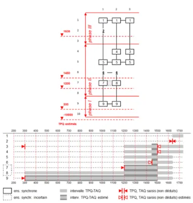
Figure 11. Stratigraphic time (left) and historical time (right); the historically  dated  house  B  has  a  “certain  use  time”  provided  by  historical documentation;  the  “possible  time”  of  the  related  stratigraphic  units  of  construction and destruction is consequently limited. 

Figure 10. If we add a phase of refitting (new floor) of the building showed in  the  example  Figure  8,  we  see  there  is  a  complex  relation  between stratigraphic  units  (and  their  groupings)  and  material  entities  in  the historical  time  (and  their  groupings):  the  same  unit  (3)  is  related  to  two  successive historical (use time) phases. 

can infer that this group 10 belongs to a historic material entity: the building with its use duration after its construction and before its destruction (B). Let us admit that this building is mentioned in two documents dated 1710 and 1790. These documents directly give a slot of certain time for this house as historical entity (between 1710 and 1790). In other words, if we consider the inaccuracy intervals applied to this historical entity (and not to the stratigraphic units), these documents give directly the beginning at the latest and the end at the earliest of this entity (BlB = 1710; EeB= 1790). The other endpoints may

come from related stratigraphic units: the beginning at the earliest from the stratigraphic group (SG 10) and the end at the latest from the destruction unit (2) logically limit the B entity timespan; so BeB = 1600 ; ElB= 1860.

We can transfer these historical dating indications to the related stratigraphic units, but not to the same endpoints. The earlier document gives logically 1710 as the end at the latest to the stratigraphic group SG 10 (and thus to the prior units) because if the building is mentioned as existing, its construction is already achieved; reciprocally, the later document gives 1790 as the beginning at the earliest to the destruction cut 2 (because if the building is mentioned as existing, its destruction has not begun yet).

We can see again that stratigraphic and historic times are not the same: this interval [1710, 1790], which is a certain timespan for a material entity in the historical time, is, on the other hand, a gap in the stratigraphic quantified time because no observed occupation stratigraphic unit corresponds to the use time of this historical entity.

6. DEALING WITH UNCERTAIN DATING: THE ESTIMATED  TIME 

As said above, we have to deal with uncertainty at each step of the chronological reasoning.

We saw that inaccuracies of dating result in a kind of uncertainty (“possible time”) linked to the formation of a stratigraphic unit – or to the use time of a historical or functional entity. Furthermore, if we admit an uncertain modality for stratigraphic relationships (cf. Section 2.3), and more generally for succession time constraints, it must be logically extended to the quantified frame of time by a distinction between “certain” and “estimated” (understood as uncertain) quantified time data. A double system of intervals (certain and estimated) is then necessary. The estimated intervals, more accurate but hypothetical, are limited by the certain ones. They result in an intermediary “estimated” time between the “possible” and the “certain” time (Figure 12).

The advantage is a more flexible process, able to take in account uncertain observations; but also to take in account indications, more often hypothetical than certain, about the temporality of the objects found in the units, involving their use time and notions such as “primary deposit” or “closed find”.

For instance, the graph (Figure 13) shows the dating of our example if we add this assuming about the coin dated 1600 found in the layer 3: it is a primary deposit, and it is not very worn, so that its circulation duration before its deposit is probably less than 50 years after its minting date.

For any dating element, we have to ask clearly the question: what endpoint is informed by this indication? Here, it is not an estimated TPQ, but an estimated beginning at the latest. Indeed, this maximum estimated duration since the TPQ and before the deposit gives directly an estimated beginning at the latest for the unit 3, because the formation of the unit 3 has necessarily already begun when the coin is deposited. So we can write: eBl3

= 1649 (estimated beginning at the latest of unit 3 = minting date of the coin added to less than 50 years). Then, as we have admitted a duration at the longest for the unit 3 (Dl3 = 1 cf.

Section 3.4), we get an estimated end at later for the unit 3: eEl3

= 1649 +1 = 1650 (cf. inequation (8) above). This deduced estimated TAQ defines an “estimated time” – more accurate, but less certain than the “possible time” – for the unit 3 and the stratigraphically related units and groups.

Another utility of this notion of “estimated time” is to deal with the heterogeneous quality of the documentation which sometimes characterizes the archaeological field data, and which inevitably affects the researches using various sources to identify historical and functional entities (especially at the wider scale of an archaeological map). Such a chronological frame including estimated inaccuracy intervals is experimented by J. Gravier in a current research about the city of Noyon (France) at this wider scale of urban historical and functional entities [33].

Finally, it is also a way to display a chosen chronological hypothesis, between the two extreme possible chronologies, at the earliest and at the latest.

7. PRACTICAL APPLICATIONS: COMPUTERIZED TOOLS 

The approach presented here needs computing tools, because, if the underlying formalization is simple, the calculations – particularly the manipulation of the complete system of inaccuracy intervals – are quite boring manually. There again, it is a work in progress, and the complete integration of the process within a single application is not finished yet. Nevertheless, two applications already exist and allow handling automatically a wide part of the process.

The first one is Le Stratifiant: a stratigraphic data processing application developed since 2005, as an add-on to the Microsoft Excel software [6], [7]. Its functionalities include stratigraphic graphs generation from sets of data (units and relationships)

Figure  12.  “Estimated  time”  provided  to  a  unit  i  (between  an  estimated beginning  at  the  earliest  eBe  and  an  estimated  end  at  the  latest  eEl)  if 

entered by the user or imported from a database, uncertain relationships processing, and logical faults detection. It also performs limited processing of units grouping (phasing) and inaccuracy intervals of quantified dating (Figure 14). Its use in operational conditions since a few years by some French archaeologists (in the Institut de recherches archéologiques preventives [34], Bibracte archaeological center, or territorial archaeological units) has provided some experience feedbacks.

In its present state, this application does not include subset relationships processing nor extended dating intervals (other

than [TPQ-TAQ]) processing. The development of a new version containing these features has begun.

From now, an experimental simple tool – Chronophage – has been developed in order to explore the calculation of all the inaccuracy dating intervals of a unit (stratigraphic unit or historic entity), on the free software LibreOffice /OpenOffice Calc. It contains formula to solve inequations and to reduce the intervals from known endpoints and default values chosen by the user. It is not yet integrated in Le Stratifiant and it doesn’t process stratigraphic relationships (or relative time constraints); but for each unit, it detects logical faults of dating, gives the possible, certain and/or estimated time; and it provides quantified time graphs (Figure 15Chronophage tool (formulas and macros in LibreOffice Calc free software)).

These tools are free and available (in French) at:

https://cours.univ-paris1.fr/fixe/03-40-doctorat-archeologie-atelier-sitrada (section: “outils téléchargeables”).

8. CONCLUSION 

This is only a preliminary paper: beyond the description of the approach briefly presented here, it is necessary to test it with real and enough numerous data. It will be the next step of our work, using the computerized tools presented above and their current developments. In a further step, other developments are possible: especially the application of such a systematic approach using inaccuracy intervals to the temporality of the archaeological objects (and not only to the contexts).

Finally, this work in progress is an attempt to explicit basic steps of the chronological reasoning, upstream to the advanced chronological modelling. Indeed, these basic steps, that are fundamental, remain often implicit and ambiguous. Formalizing them – as simply as possible – is a practical issue, in order to get some computer-based aids; it is also a methodological and epistemological issue, in order to make our chronological statements more rigorous and explicit.

Figure 14. Le Stratifiant: stratigraphic graph with phases and TPQ thresholds (up); TPQ‐TAQ intervals graph (down). 

REFERENCES 

[1] E. Harris, The laws of archaeological stratigraphy, World Archaeology, 11-1 (1979), pp. 111-117.

[2] E. Harris, Principles of Archaeological Stratigraphy, Academic Press, London, 1989, ISBN 978-0-12-326651-4.

[3] P.-R. Giot, L. Langouët, La datation du passé - la mesure du temps en archéologie, Revue d’Archéométrie, supplément (1984). [4] A. Ferdière, “Comment datent les archéologues (et

céramologues) - révision d’une question de méthode”, in: Abécédaire pour un archéologue lyonnais : Mélanges offerts à Armand Desbat. S.Lemaître, C.Batigne-Vallet (editors), Editions Mergoil, Autun, 2015, ISBN 978-2-35518-049-1, pp. 47-54. [5] A. Lehoërff, “Les enjeux de la construction du temps en

archéologie”, in: Construire le temps- histoire et méthodes des chronologies et calendriers des derniers millénaires avant notre ère en Europe occidentale. Bibracte, Glux-en-Glenne, 2008, ISBN 978-2-909668-60-4, pp. 9-16.

[6] B. Desachy, Le Stratifiant - un outil de traitement des données stratigraphiques, Archeologia e calcolatori, 19 (2008), pp.187-194. [7] B. Desachy, De la formalisation du traitement des données

stratigraphiques en archéologie de terrain, Phd thesis, Université Panthéon-Sorbonne Paris I, 2008, https://tel.archives-ouvertes.fr/tel-00406241/document

[8] B. Desachy, Formaliser le raisonnement chronologique et son incertitude en archéologie de terrain, Cybergeo: European Journal of Geography, 597 (2012), URL:

http://cybergeo.revues.org/25233

[9] B. Desachy, “A simple way to formalize the dating of stratigraphic units”, Proc. of the 42nd Annual Conference on Computer Applications and Quantitative Methods in Archaeology, 2014, Paris, France (2015) pp. 365-369.

[10] C. Orton, Mathematics in Archaeology, Cambridge University Press, Cambridge, 1982, ISBN 978-0-521-28922-1.

[11] J.S. Taylor, “Timing things right - stratigraphy and the modelling of intra-site spatiotemporality using GIS at Çatalhöyük”, paper presented at 42nd Computer Applications and Quantitative Methods in Archaeology (CAA) Conference, 22nd - 25th April, Paris, France, 2014.

[12] B. De Roo, C. Stal, B. Lonneville, A.De Wulf, J. Bourgeois, P. De Maeyer, Spatiotemporal data as the foundation of an archaeological stratigraphy extraction and management system, Journal of Cultural Heritage, accepted 2015, doi:10.1016/j.culher.2015.12.001.

[13] I. Herzog, “Possibilities for analysing stratigraphic data”, PDF file on CD. Phoibos Verlag, Vienna, 2002.

[14] C. Traxler, W. Neubauer, “The Harris Matrix composer - a new tool to manage archaeological stratigraphy”, in: Archäologie und Computer - Kulturelles Erbe und Neue Technologien - Workshop 13 3-5 November 2008, W.Börner, S.Uhlirz S. (Editors), PDF file on CD, Phoibos Verlag, Vienna, 2009. [15] B. Desachy, F. Djindjian, Sur l’aide au traitement des données

stratigraphiques des sites archéologiques, Histoire & Mesure, 5-1 (1990), pp.51-88.

[16] I. Herzog, “Computer-aided Harris Matrix generation”, in: Practices of Archaéological Stratigraphy, E. C Harris, M. Brown, G. Brown (Editors), Academic Press, London, 1993, pp.201‑ 217.

[17] J.G. Degos, Les méthodes d'ordonnancement de type PERT et MPM - quelques éléments essentiels, Techniques économiques,

Institut National de Recherche et de Documentation Pédagogique, 81 (1976), pp.19-24.

[18] S. Roskams, Excavation, Cambridge University Press, Cambridge, 2001, ISBN 978-0-521-35534-6.

[19] M. Carver, Archaeological investigation, Routledge, London, 2009, ISBN 978-0-415-48918-8.

[20] I. Herzog, J. Hansohm, “Monotone regression – a method for combining dates and dtratigraphy”, PDF file on CD. Phoibos Verlag, Vienna, 2008.

[21] L. Bellanger, R. Tomassone, P. Husi, A statistical approach for dating archaeological contexts, Journal of Data Science, 6-2 (2008), pp.135‑54.

[22] P. Lanos, P. Dufresne, “Modélisation statistique bayésienne des données chronologiques”, in: L’Archéologie à Découvert. S.A. de Beaune, H.P. Francfort (Editors), CNRS Editions, Paris, 2012, ISBN 978-2-271-07142-2, pp. 238-248.

[23] A. Carandini, Storie Della Terra: Manuale di Scavo Archeologico, Einaudi, Torino, 2000, ISBN 978-88-06-15669-5.

[24] B. Randoin (ed.), Enregistrements des Données de Fouilles Urbaines – Première Partie, Centre national d’archéologie urbaine, Tours, 1987.

[25] I. Sharon, Partial order scalogram analysis of relations—a mathematical approach to the analysis of stratigraphy, Journal of Archaeological Science 22-6 (1995) pp. 751-767.

[26] A. Carandini, “Nuove riflessioni su “storie dalla terra”, in: Lo Scavo Archeologico - dalla diagnosi all'edizione, R.Francovich, D.Manacorda (editors), All’insegna del giglio, Firenze, 1990, ISBN 88-7814-068-6, pp. 31-42.

[27] I. Herzog, “Group and conquer -, a method for displaying large stratigraphic data sets”, in: Enter the Past. The E-way into the Four Dimensions of Cultural Heritage, British Archaeological Reports Int. Ser. 1227 (2004), pp. 423-426.

[28] M. Schiffer, Formation Processes of the Archaeological Record, University of Utah Press, Salt Lake City, 1987, ISBN 978-0-87480-513-0.

[29] M. Carver, Digging for data: archaeological approaches to data definition, acquisition and analysis, in: Lo Scavo Archeologico - dalla diagnosi all'edizione, R.Francovich, D.Manacorda (editors), All’insegna del giglio, Firenze, 1990, ISBN 88-7814-068-6, pp.45-120.

[30] P. Paice, Extensions to the Harris matrix system to illustrate stratigraphic discussion of an archaeological site, Journal of Field Archaeology, 18-1 (1991) pp. 17‑28.

[31] J. Collis, “Constructing chronologies: lesson from the Iron Age”, in: Construire le Temps- histoire et méthodes des chronologies et calendriers des derniers millénaires avant notre ère en Europe occidentale, A.Lehoërff (editor), Bibracte, Glux-en-Glenne, 2008, ISBN 978-2-909668-60-4, pp.85-104.

[32] X. Rodier, L. Saligny, Modélisation des objets historiques selon la fonction, l’espace et le temps pour l’étude des dynamiques urbaines dans la longue durée, Cybergeo: European Journal of Geography, 502 (2010), URL: http://cybergeo.revues.org/23175

[33] J. Gravier, “Recognize temporalities from formalization of dating urban units: three case studies”, Proc. of 42nd _{Annual Conference}

on Computer Applications and Quantitative Methods in Archaeology, 2014, Paris, France, (2015) pp.371-379.

[34] A. Bolo, M. Muylder, C. Font, T. Guillemard, De la tablette PC à la cartographie de terrain: exemple de méthodologie sur le chantier d’archéologie préventive de Noyon (Oise), Archeologia e Calcolatori, supplemento 5 (2014), pp. 247-256.