HAL Id: cirad-00168356
http://hal.cirad.fr/cirad-00168356
Submitted on 27 Aug 2007
HAL is a multi-disciplinary open access
archive for the deposit and dissemination of
sci-entific research documents, whether they are
pub-lished or not. The documents may come from
teaching and research institutions in France or
abroad, or from public or private research centers.
L’archive ouverte pluridisciplinaire HAL, est
destinée au dépôt et à la diffusion de documents
scientifiques de niveau recherche, publiés ou non,
émanant des établissements d’enseignement et de
recherche français ou étrangers, des laboratoires
publics ou privés.
Province
van Cu Pham, Chu Xuan Huy, Nguyen Thi Thuy Hang, Thapa R. B.,
Frederic Borne
To cite this version:
van Cu Pham, Chu Xuan Huy, Nguyen Thi Thuy Hang, Thapa R. B., Frederic Borne. Using
multi-temporal satellite images to evaluate the changes of vegetation index of land cover in Thai Binh
Province. V.Porphyre Nguyen Que Coi. Pig Production Development, Animal-Waste Management
and Environment Protection: a Case Study in Thai Binh Province, Northern Vietnam, CIRAD-PRISE
publications, pp.37-54, 2006. �cirad-00168356�
Satellite images highlight the existing situation and expected threats against environment. The integration of maps displaying vegetation and urban indices with statistic data on pig production allows us to make clear the relation between land cover changes and pig production development in Thai Binh.
Satellite Images to Evaluate
the Changes of Vegetation
Index of Land Cover
in Thai Binh Province
Pham Van Cu, Chu Xuan Huy, Nguyen Thi Thuy Hang, Rajesh Bahadur Thapa, Frédéric Borne
Introduction
The spatial analysis introduced in this study contributes to identify the relationship between traditional agricul-tural practice and pig production activities at the provincial scale. Most of the studies carried out in the frame-work of our project used local statistic and cartographic data in accepting their heterogeneity in their reliability and their standards (see next chapters). Under this circumstance, the use of multi-temporal remotely sensed data will contribute to complete the lack of data in some cases and to provide another vision to understand the spatio-temporal evolution of the land cover in Thai Binh through a series of vegetation indices extracted from the images. The vegetation indices computed for the whole image are associated to communal administrative map of Thai Binh to create a time series of vegetation indices of each commune. The integration of maps dis-playing the vegetation indices with statistic data on pig production allows us to make clear the relation between land cover changes and pig production development in Thai Binh.
The current research aims to highlight the existing situation and expected threats against environment. This pre-liminary work will be the base for a decision making and strengthening tool for the Thai Binh's authorities in order to define urgently suitable technologies for land-use and investment planning, and to enforce the regulation con-sidering environment. For this purpose, a series of multi-temporal satellite imageries are used to extract the vegetation index of the whole province for a period between 1975 up to 2003 in depending upon the availability of satellite images.
Material and methods
Used data
Satellite Images - Four Landsat images (1MSS, 1TM and 2 ETM+7 acquired respectively in November 1975, November 1989, September and November 2001) and three scenes of ASTER images (one in
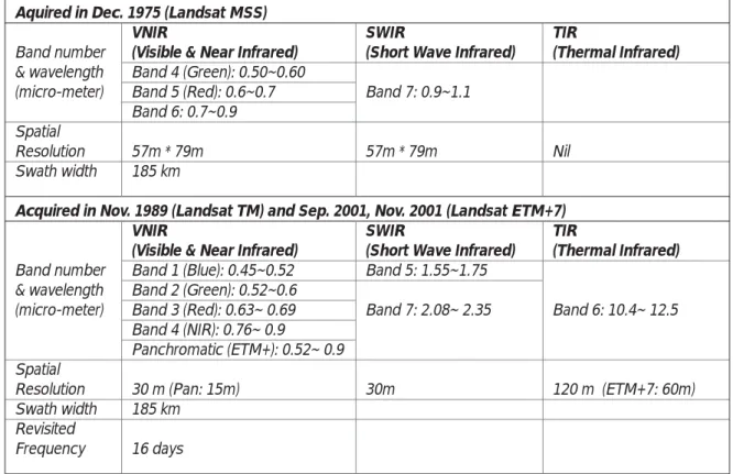
September 2002 and two in November 2003) were obtained for the study areas. The tables 1 and 2 present Landsat and ASTER data specifications respectively.
Ancillary data are supplied by administrative maps of Thai Binh and statistic yearbook on fertilizer con-sumption of Thai Binh
Table 1: Specification of Landsat data
Band number & wavelength (micro-meter) Spatial Resolution Swath width Band number & wavelength (micro-meter) Spatial Resolution Swath width Revisited Frequency VNIR
(Visible & Near Infrared)
Band 4 (Green): 0.50~0.60 Band 5 (Red): 0.6~0.7 Band 6: 0.7~0.9 57m * 79m 185 km VNIR
(Visible & Near Infrared)
Band 1 (Blue): 0.45~0.52 Band 2 (Green): 0.52~0.6 Band 3 (Red): 0.63~ 0.69 Band 4 (NIR): 0.76~ 0.9 Panchromatic (ETM+): 0.52~ 0.9 30 m (Pan: 15m) 185 km 16 days SWIR
(Short Wave Infrared)
Band 7: 0.9~1.1
57m * 79m
SWIR
(Short Wave Infrared)
Band 5: 1.55~1.75 Band 7: 2.08~ 2.35 30m TIR (Thermal Infrared) Nil TIR (Thermal Infrared) Band 6: 10.4~ 12.5 120 m (ETM+7: 60m)
Aquired in Dec. 1975 (Landsat MSS)
Acquired in Nov. 1989 (Landsat TM) and Sep. 2001, Nov. 2001 (Landsat ETM+7)
Table 2: Specification of ASTER (Advanced Spaceborne Thermal Emission and Reflectance Radiometer) data
Band number & wavelength (micro-meter) Spatial Resolution Swath width Revisited Frequency VNIR
(Visible & Near Infrared)
Band 1 (Green): 0.52~0.60 Band 2 (Red): 0.63~0.69 Band 3N (NIR): 0.76~0.86 15m 60 km 16 days SWIR
(Short Wave Infrared)
Band 4: 1.600~1.700 Band 5: 2.145~2.185 Band 6: 2.185~2.225 Band 7: 2.235~2.285 Band 8: 2.295~2.365 Band 9: 2.360~2.430 30m TIR (Thermal Infrared) Band 10: 8.125~8.475 Band 11: 8.475~8.825 Band 12: 8.925~9.275 Band 13: 10.25~10.95 Band 14: 10.95~11.65 90m Acquired in Nov.2003
Method
Image pre-processing
Considering the available images of Thai Binh are of different acquisition dates and are acquired by different sensors (MSS, TM, +ETM and ASTER) the radiometric and geometric corrections are needed in
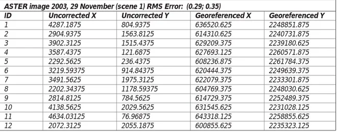
pre-processing procedures. Data providers and all the Digital Numbers were already converted into reflectance values of 32 bits by Radiometric Calibration. Geometric Correction was carried out by polynomial model using UTM WGS 84 projection. The details of Ground Control Point GCP and Root Mean Square RMS are presented in the table 3.
Landsat image ASTER image
Radiometric correction
Geometric correction
Image subset
Vegetation indices Mapping
Figure 1: Image Processing Flowchart
Table 3: GCP used for geometric correction of ASTER image 2003, 29 November scene 1
Uncorrected X 4287.1875 2904.9375 3902.3125 3587.4375 2292.5625 3219.59375 3491.5625 2202.34375 2814.8125 4138.5625 4634.03125 2072.3125 ID 1 2 3 4 5 6 7 8 9 10 11 12 Uncorrected Y 804.9375 1563.8125 1515.4375 121.6875 236.4375 914.84375 1975.3125 1178.59375 784.5625 2029.5625 76.96875 2055.1875 Georeferenced X 636520.625 614310.625 629209.375 627693.125 608236.875 620444.375 622079.375 604769.375 614729.375 631545.625 643318.125 600855.625 Georeferenced Y 2248851.875 2240731.875 2239180.625 2260571.875 2261784.375 2249639.375 2233301.875 2248030.625 2252489.375 2231028.125 2258855.625 2235323.125
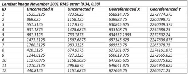
Table 6: GCP used for geometric correction of Landsat image +ETM November 2001 Uncorrected X 912.0625 1646.9375 104.8125 811.375 1733.5625 467.4375 1371.3125 1698.0625 1063.9375 416.3125 1328.3125 448.9375 ID 1 2 3 4 5 6 7 8 9 10 11 12 Uncorrected Y 1054.1875 438.5625 299.9375 289.375 1321.5625 834.0625 1584.6875 959.4375 510.1875 510.4375 1054.9375 1152.9375 Georeferenced X 641173.75 662111.25 618146.25 638271.25 664588.75 628505.625 654289.375 663594.375 645489.375 627029.375 653038.75 627991.25 Georeferenced Y 2263341.25 2280911.25 2284841.25 2285158.75 2255743.75 2269595.625 2248229.375 2266059.375 2278854.375 2278843.125 2263318.75 2260541.25
Landsat image November 2001 RMS error: (0.34, 0.38)
Table 4: GCP used for geometric correction of ASTER image 2003, 29 November scene 2
Uncorrected X 3488.4375 2429.1875 4128.0625 2139.6875 2005.4375 4484.84375 3466.40625 2909.03125 4404.5625 3744.09375 ID 1 2 3 4 5 6 7 8 9 10 Uncorrected Y 2228.4375 2806.0625 3880.6875 3861.9375 2158.4375 2685.03125 3274.40625 4104.09375 3158.9375 3915.34375 Georeferenced X 634396.875 617391.875 640151.25 610714.375 612559.0625 648144.6875 631710.3125 621576.875 645885.9375 634380.9375 Georeferenced Y 2288654.375 2282468.125 2262701.25 2267474.375 2293037.187 2279624.063 2273184.063 2262146.875 2272780.938 2263057.812
ASTER image 2003, 29 November (scene 2) RMS Error: (0.25; 0.28)
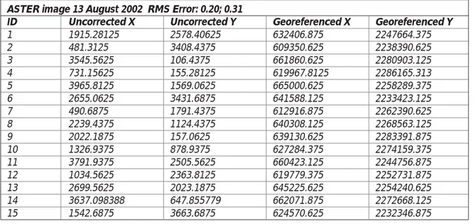
Table 5: GCP used for geometric correction of ASTER image 31 August 2002
Uncorrected X 1915.28125 481.3125 3545.5625 731.15625 3965.8125 2655.0625 490.6875 2239.4375 2022.1875 1326.9375 3791.9375 1034.5625 2699.5625 3637.098388 1542.6875 ID 1 2 3 4 5 6 7 8 9 10 11 12 13 14 15 Uncorrected Y 2578.40625 3408.4375 106.4375 155.28125 1569.0625 3431.6875 1791.4375 1124.4375 157.0625 878.9375 2505.5625 2363.8125 2023.1875 647.855779 3663.6875 Georeferenced X 632406.875 609350.625 661860.625 619967.8125 665000.625 641588.125 612916.875 640308.125 639130.625 627284.375 660423.125 619779.375 645225.625 662071.875 624570.625 Georeferenced Y 2247664.375 2238390.625 2280903.125 2286165.313 2258289.375 2233423.125 2262390.625 2268563.125 2283391.875 2274159.375 2244756.875 2252731.875 2254240.625 2272668.125 2232346.875
Index Computing
Vegetation index (VI) is one of the physical indices we can compute from the spectral bands of remote sensing image. The vegetation index VI is used in dif-ferent applications such as canopy and biomass esti-mation, crop monitoring and drought monitoring etc. In the literature, other VI are cited and differ in terms of spectral bands and the algorithms and in terms of application (Rouse et al 1974; Colwell et Suits 1975;
Huete, 1988; Richardson and Wiegand 1977; Baret et al. 1989; Kaufman et Tanré, 1992 ; Qi et al 1994). The paragraphs bellow describe some of these indices used for our study.
SAVI (Soil Adjusted Vegetation Index) computes the ratio between red and near infrared spectral region with some added terms to adjust for different bright-ness of background soil (Huete, 1988). Due to paddy
Table 7: GCP used for geometric correction of Landsat image +ETM September 2001
Uncorrected X 840.1875 413.3125 913.3125 976.625 1765.4375 95.625 358.1875 ID 1 2 3 4 5 6 7 Uncorrected Y 1368.8125 372.8125 1053.4375 235.875 1060.6875 337.625 857.6875 Georeferenced X 639113.75 626908.75 641172.5 642951.25 665473.125 617856.25 625373.75 Georeferenced Y 2254381.25 2282751.25 2263347.5 2286676.25 2263166.875 2283783.75 2268961.25
Landsat September 2001 RMS error: (0.37, 0.58)
Table 9: GCP used for geometric correction of Landsat image MSS December 1975
Uncorrected X 857.875 636.625 1153.625 80.875 1106.375 1745.625 1213.875 ID 1 2 3 4 5 6 7 Uncorrected Y 1132.375 701.875 556.625 379.625 1288.125 898.875 923.375 Georeferenced X 639605.625 633274.375 647997.5 617393.75 646698.125 664921.875 649768.125 Georeferenced Y 2261036.875 2273323.125 2277472.5 2282466.25 2256586.875 2267711.875 2267011.875
Landsat December 1975 RMS error: (0.41, 0.50)
Table 8: GCP used for geometric correction of Landsat image TM November 1989
Uncorrected X 1535.3125 869.625 551.3125 631.1875 681.3125 1473.3125 1768.3125 426.3125 1244.8125 1127.6875 1210.3125 440.8125 ID 1 2 3 4 5 6 7 8 9 10 11 12 Uncorrected Y 723.5625 1158.125 117.9375 1428.6875 733.1875 1597.6875 983.3125 674.9375 727.3125 1158.5625 296.6875 1151.6875 Georeferenced X 658914.375 639928.75 630845.625 633108.75 634552.1995 657145.625 665553.75 627281.875 650619.375 647295.625 649641.875 627696.25 Georeferenced Y 2272774.375 2260398.75 2290039.375 2252686.25 2272502.24 2247836.875 2265378.75 2274161.875 2272665.625 2260375.625 2284950.625 2260571.25
harvested time ends in October, the result of SAVI images during November-December presents the situation of natural vegetation in the province. The SAVI image of September helps to understand the agricultural activities in details. The Normalized Differential Water Index (NDWI) estimates the situa-tion of water in the province. The ratio between red and Short Wave Infrared (SWIR) spectral region clearly enhanced water bodies to the brighter pixels (CPM, 2003).
Where: p is the reflectance, L~ 0.5
Where:
And
Bare Soil Index (BI) was also computed to identify
dif-ference between agriculture and none agriculture vegetation. The bare soil, fallow lands, and vegetation (with marked background response) are enhanced when using the BI index (Jamalabad and Abkar, 2004).
As for 2003, the non-vegetation objects are addi-tionally extracted from Urban Index UI (Kawamura, M., S. Jayamamana and Y. Tsujiko 1997) to emphasize the vegetation presence and UI is very helpful to dis-criminate vegetation and non-vegetation land cover types. The UI is calculated as following:
For Landsat MSS, we compute pnirfrom band 3 and
predfrom band 2. For Landsat TM and ETM+, pniris computed from band 4, pred from band 3, pswirfrom band 5 and pswir2from band 7, pbluefrom band 1. For ASTER, pred, pnir, pswir, pswir2are taken from band 2, 3, band 4, band 5 respectively. All the equations above provide value ranges from -1 to +1. To avoid negative value in further analysis, we have added +1 in each
Where:
Grey level value after calibration Orginal grey level value to be calibrated
Stretching co-efficient for the set of pixel to be calibrated
Shifted co-efficient for each pixel
Maximum grey level value of pixels in the stan-dard image
Minimum grey level value of pixels in the standard image
Maximum grey level value of pixels in the dependent image
Minimum grey level value of pixels in the dependent image
In this study, we used the value extracted from the image Landsat ETM+7 acquired in November 2001 as the reference.
equation. Thus, the resulted images will have value between 0~2 where higher value show the existence of the environment parameters (i.e. high in SAVI shows high in vegetation, high in NDWI shows high in water). We compute also mean and standard deviation from each index at commune level to analyze the environ-mental situation with socio-economic condition at each commune.
Scaling problem and solution
As explained in previous sector of this report, due to the difference of acquisition dates and especially, to the spectral band difference, the VI values computed for ASTER images vary between 0.80131286 and 1.18813098 meanwhile the range of VI computed for Landsat images is in between 0.64208417 and 1.09550542. In order to compare these values we need to scale the ASTER VI values to fit the Landsat VI range using relative scaling method. This method is described by the formula:
Results
Multidate statistical variations of indices
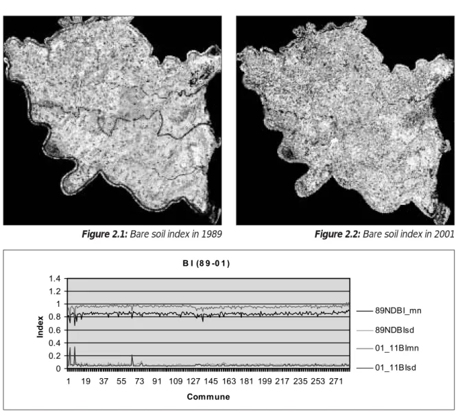
SAVI, BI, NDWI and UI indices were computed in multi-temporal Landsat images and ASTER images (see fig. 2.1 to 2.19). The multidate statistical variations of com-puted indices are used to analyze the environmental changes with respect to vegetation, agriculture, water and urban activities. The indices after calibration have produced relative results based on electromagnetic spectrum recorded in the images. The mean score and coefficient of standard deviation of each index were carefully evaluated at commune level. Standard devi-ation of mean helped to understand the distribution pattern of the objects in the land surface.Principally, the SAVI appears brighter in healthy vege-tation areas whereas BI seems brighter in bare land areas. The high NDWI corresponds to the areas with high water content. The variation of UI index indicates the different density of urban and built areas.
The SAVI index of 1975, 1989, 2001, 2003 represent the natural vegetation coverage in brighter areas. It is because of seasonal variance in agriculture practice. The high content of chlorophyll can be observed in paddy field in September. The paddy harvest is com-pleted at the end of October. Therefore, harvested paddy fields on the images taken during November and December have a high bare soil index BI and appear in brighter pixels.
Some inconsistencies in distribution pattern of the mean of SAVI are observed in some communes. Decreasing trend of natural vegetation is observed in past three Bare soil index of 2001 is also getting lower as compared to year 1989. Mean distribution of the bare soil index seems more consistent as compared to SAVI mean. Comparison of BI with SAVI makes sense of conventional agriculture occupancy as well as practices. There are not so much fluctuations in distri-bution of objects in BI. Decreasing patterns in SAVI and BI exposed the decreasing of conventional agriculture practices (i.e. paddy).
The result of NDWI is quite different than SAVI and BI. Increasing pattern is observed in water bodies although inconsistency in distribution of the water bodies is found in some communes.
Several farmers in the province are changing their tra-ditional agriculture land to modern aquatic practices. It is one of the major factors that increased the water properties and reduced the vegetation properties as compared to 1980s. Direct relation of fish farms to the pig production was observed during the field visit. Pig waste is being used as a source of input for aquatic farming fertilization of ponds, nutrient for fishes. Thanks to the high demand of lean pork meat in the growing cities and flexible government policies, farmers are attracted to the integrated agriculture prac-tices (pig and fish ponds).
There is very good compromise between water and urban index. Most of the urban areas are observed along the water bodies like rivers, canals and lakes. The increased urban activities in the province do not have significant impact in reducing water properties. But it has significant impact in reducing the vegetation. The UI mean increased as a peak in some communes whereas the SAVI mean decreased just like a gorge in the corresponding communes. So, the land of agricul-ture is being occupied by urban function. The conver-sion of agriculture land to urban uses is natural eco-nomic process in widely observed in Thai Binh. Relation between vegetation activities and urban func-tion was checked in September 2001 results and found correlation coefficient at -0.606. It has strong negative linear relation between the UI and SAVI mean, which suggest the urban activities replacing the natural environment significantly.
Vegetation is thus getting sparse day by day because of growing urban activities, integrated agriculture prac-tices, government priorities on intensification of pig production and aquatic products.
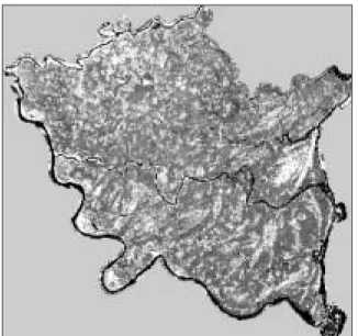
Figure 2.1: Bare soil index in 1989 Figure 2.2: Bare soil index in 2001
Figure 2.3: Bare soil index from 1989 and 2001 (mn – mean, sd- standard deviation)
Figure 2.6: SAVI in 2001, November
Figure 2.8: SAVI from Landsat image (1975 – 2001) and ASTER image (2003) at harvested season. Zero value
is considered for communes from 1 to 116 due to the lack of image (mn- mean, sd-standard deviation)
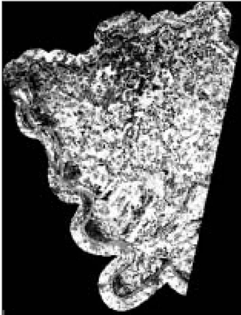
Figure 2.7: SAVI in November 2003
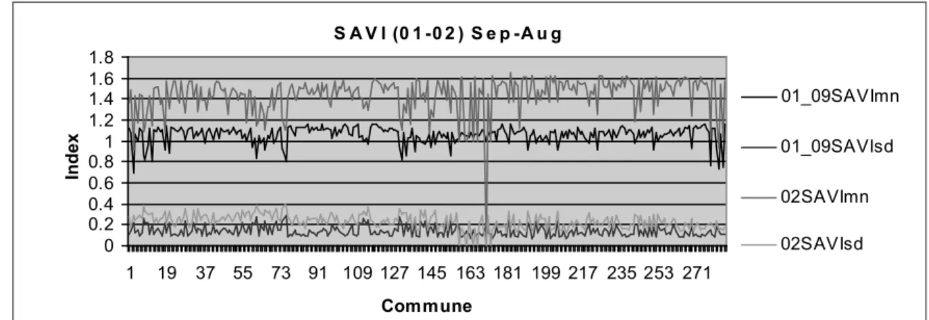
Figure 2.11: SAVI in farming season taken from Landsat image and ASTER image. The SAVI values from
ASTER image are particularly high due to influence of cloud (mn- mean, sd- standard deviation)
Figure 2.12: NDWI in November 1989 Figure 2.13: NDWI in 2001, September
Figure 2.16: NDWI from 1989 to 2003. NDWI from 2003 is considered 0 for 1st -116th ordered communes
owing to the lack of image covering them (mn-mean, sd- standard deviation)
Figure 2.19: UI from 2001 to 2003 (mn- mean, sd- standard deviation) Figure 2.17: UI from Landsat 2001, September Figure 2.18: UI from ASTER 2003, November
Cartographic Representation of results
Due to the limits in statistic data, we cannot make a full representation of all physical index. The geo-referenced index images are crossed with the administrative map of Thai Binh to produce the normalized biophysical indices map at communal level, i.e., each commune ofThai Binh is now characterized by a series of Vegetation Index. The results are presented in a cartographic data-base of which the attribute data describing the com-puted indices are organized in relational model and very easy to manipulate in GIS environment.
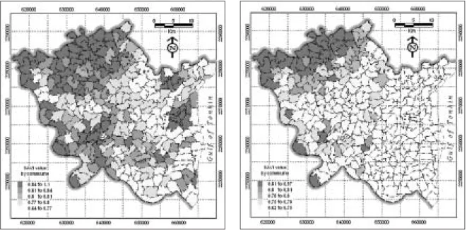
Mean SAVI (Soil Adjusted Vegetation Index) Map by Commune
Figure 3.1: SAVI in December 1975 Figure 3.2: SAVI in November 1989
The SAVIs are extracted from Landsat and ASTER data, which were acquired during the harvesting season (Novembers). To facilitate the analysis, the SAVI mean values are associated to each commune and this value represents mean SAVI of the whole com-munal territory. As mentioned above, the scaling of SAVI values of the two dates of Landsat and ASTER data allows comparisons each with other. The higher communal SAVI the larger vegetation cover is (fig. 3). Due to its scene limitation, ASTER data covers only a part of Thai Binh and no value is computed for the non-data area.
As the Landsat and ASTER data are acquired in the period of similar climate conditions the atmospheric influence is negligible. The very low value of SAVI
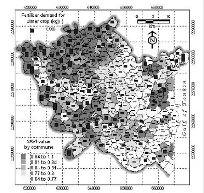
extracted from MSS data can be explained by its low spatial resolution (57m*79m) and bandwidths. For the period from 1989 to 2003, the high SAVI values are concentrated in the Western and North West com-munes of Thai Binh even if the acquisition dates coin-cided to the harvest period. This phenomena may be explained by the presence of other cultures than rice in this period (for example vegetable, soya-bean etc.) which have been planted just after the harvest. To check this hypothesis, we used the statistic data on communal fertilizer consummation for winter plants and have found the high correlation between the con-sumption/use of fertilizer and SAVI values in these communes (Fig.4).
Mean NDWI (Normalized Difference Water Index) Map by Commune
Figure 5.1: NDWI in November 1989 Figure 5.2: NDWI in November, 2001
NDWI was introduced by Gao (1996) to assess water content in a normalized way. This index increases with vegetation water content or from dry soil to free water. For the reference, we take the Land Use Map of 2000, the closest to Landsat image acquisition date we can have. The low NDWI values extracted from the Landsat TM and +ETM images acquired during dry season (November) of 1989 and 2001 indi-cate the low water content in soil and vegetation in the North West sector of the province. However, there observed a big difference in NDWI in the rest of terri-tory in these two dates (Fig. 5.2, 5.3). This difference is thought related to the change of land use from rice in 1989 to Winter Crop in 2001.
The NDWI computed for ASTER image (Fig. 5.3) cap-tured in November 2003 that covers only the West part of Thai Binh are low and corresponds to the area of Winter Crop.
In general, the NDWI values of North West Communes are lower than in other places (fig. 5.1 to 5.3) and showing the dryer soil conditions. In spite of that, their SAVI values indicate the existence of some vegetation (fig. 3.1 to 3.4) supposed to be winter vegetables as shown in Land Use Map (fig.7). These communes are mainly characterized by a high topography (see Chapter 2) and poorly irrigated terrain. Figure 6 shows the coincidence of winter crop and permanent vege-tation (presented in black) with the areas of low NDWI values (between 0.937 and 1.102).
Conclusion
Different physical indices extracted from a time series of satellite images between 1975 and 2003 allow char-acterizing the changes of land cover in Thai Binh in this period. Based on SAVI, UI and BI indices change eval-uation, the surface of winter crop appeared to decrease gradually and concentrate mainly in suburb communes of Thai Binh City and the adjacent com-munes of Vu Thu and Dong Hung Districts.
The communes having high NDWI (1.102~1.263) have been reduced in the period 1989-2003. The brutal decrease of NDWI scale computed for ASTER image have highlighted the difference in spatial and spectral resolution of this sensor; this is to be verified by ancil-lary statistic data.
Comparison between SAVI and NDWI values eva-luated the spatial repartition of dry season land cover
types; where the high SAVI values (0.8-1.1) coincide with low values of NDWI (0.937-1.102), we can observe the presence of winter crop. This inverse rela-tion could be used to monitor the winter crop in dry season.
For the first time, we have found a good correlation between fertilizer demand statistics and high values of SAVI which indicate the high demand in fertilizer of North West communes where the winter crop are pre-dominant in dry season.
The integration of SAVI, NDWI, UI and BI on the admi-nistrative map with communal boundaries of Thai Binh provides a good tool for spatial analysis of multi-tem-poral changes of land cover characteristics and for analyzing spatial correlation between these characte-ristics and other socio-economic data we may have in Thai Binh
References
1. Arbelo Rodríguez, C.D., A. Rodríguez Rodríguez, J.A. Guerra García and J.L. Mora Hernández, (2002), Soil Quality and Plant Succession in Forest Andosols, 12th ISCO Conference, Beijing, pp 452- 458.
2. Baret F.G., G. Guyot and D.-J. Major, 1989. A vegetation index which minimizes soil brightness effects on LAI and APAR estimation, 12th Canadian Symposium on Remote Sensing, Canadian Remote Sensing Society, Vancouver, p. 1355-1358.
3. Barnes, E.W., K.A. Sudduth, J.W. Hummel, S.M. Lesch, D.L. Corwin, C. Yang, C.S.T. Daughtry and W.C. Bausch (2003). Remote- and ground-based sensor techniques to map soil properties. Photogrammetric Engineering and Remote Sensing 69 619-630.
4. Colwell G.E. and G.H. Suits, 1975. Yield prediction by analysis of multispectral scanner data, NASA-CR 141865, ERIm 109600-17-F, NASA.
5. Huete, A.R., 1988. Asoil –adjusted vegetation index (SAVI), Remote Sensing of Environment, no 25, p.295-309.
6. Jamalabad, M. S. and A.A. Abkar (2004). Forest Canopy Density Monitoring, Using Satellite Images. XXth ISPRS Congress, Istanbul 12-23 July.
7. Kaufman, Y.-J. and D.-C. Tanré, 1992. Atmospherically Resistant Vegetation Index (ARVI) for EOS-MODIS, IEEE Transaction on Geoscience and Remote Sensing, vol. 30, no 2, p.261-270. 8. Kawamura, M., S. Jayamamana and Y. Tsujiko
(1997). ‘Comparison of Urbanization and Environmental Condition in Asian Cities using Satellite Remote Sensing Data’. Available online: http://www.gisdevelopment.net/aars/acrs/1997/p
s1/ps2008.shtml [Downloaded: 12 January, 2006] 9. C. López-Fand, M.T. Pard, 2002, The impact of tillage systems and machinary traffic on some soil properties and crop yield in a calcic luvisol of central Spain, 12th ISCO Conference, Beijing, pp138-143.
10. Lunetta R.S. and C.D.Elvidge, (Editors), 1998, Remote Sensing Change Detection: Environmental Monitoring Methods and Applications, Ann Arbor Press, Michigan, 318 p.
11. Palacios-Orueta, A., J. E. Pinzon, D. A. Roberts, and S. L. Ustin. (1998). “emote sensing of soil prop-erties in the Santa Monica Mountains: Hierarchical Foreground and Background Analysis.” Seventh Annual JPL Airborne Earth Science Workshop, Pasadena, CA. January 12-16, 1998.
12. Qi J., A. Chenbouni, A.R. Huete, Y.H. Kerr and S. Soroonshian, 1994. A Modified Soil Adjusted Vegetation Index (MSAVI), Remote Sensing of Environement, no 48, p. 119-126.
13. Richardson, A. and C. Wiegand, 1977. Distinguishing vegetation from soil background information, Photogrametric Engineering and Remote Sensing. No 43, p.1522-1541.
14. Rouse, J.W., R.H. Haas, J.A. Schell, D.W. Deering and J.C. Harla, 1974. Monitoring the vernal advance-ment retrogradation (Green Wave Effect) of natural vegetation, Maryland, USANASA/GFSC, Greenbelt. 15. Smith, W.N., Desjardins, R.L., Grant, B. and Lemke, R., 2002, Estimated N2O Emissions as Influenced by Agricultural Practices in Canada, 12th ISCO Conference, Beijing 2002, pp 317- 323.
16. Uno, Y., Prasher, S.O., Patel, R.M., Strachan, I.B. and Pattey, E. 2005. Development of field-scale soil organic matter content estimation models in Eastern Canada using airborne hyperspectral imagery. Canadian Biosystems Engineering/Le génie des biosystèmes au Canada 47: 1.9 - 1.14