HAL Id: ird-01224957
https://hal.ird.fr/ird-01224957
Submitted on 5 Nov 2015
HAL is a multi-disciplinary open access
archive for the deposit and dissemination of sci-entific research documents, whether they are pub-lished or not. The documents may come from teaching and research institutions in France or abroad, or from public or private research centers.
L’archive ouverte pluridisciplinaire HAL, est destinée au dépôt et à la diffusion de documents scientifiques de niveau recherche, publiés ou non, émanant des établissements d’enseignement et de recherche français ou étrangers, des laboratoires publics ou privés.
Prediction of soil organic carbon stock using visible and
near infrared reflectance spectroscopy (VNIRS) in the
field
A. Cambou, R. Cardinael, Ernest Kouakoua, Manon Villeneuve, C. Durand,
Bernard Barthès
To cite this version:
A. Cambou, R. Cardinael, Ernest Kouakoua, Manon Villeneuve, C. Durand, et al.. Prediction of soil organic carbon stock using visible and near infrared reflectance spectroscopy (VNIRS) in the field. Geoderma, Elsevier, 2015, 261, pp.151-159. �10.1016/j.geoderma.2015.07.007�. �ird-01224957�
1
Prediction of soil organic carbon stock using visible and near infrared reflectance spectroscopy (VNIRS) in the field
Aurélie Cambou, Rémi Cardinael, Ernest Kouakoua, Manon Villeneuve, Céline Durand, Bernard G. Barthès*
IRD, UMR Eco&Sols, Montpellier SupAgro, 2 place Viala, 34060 Montpellier Cedex 2, France
*corresponding author: email <bernard.barthes@ird.fr>; phone +33(0)4.99.61.21.36
Abstract
Due to the role of soils in the global carbon cycle, there is increasing demand for data on soil organic carbon (SOC) stock, but the conventional determination of SOC stock (SSOC) is tedious and hardly allows meeting this demand. Visible and near infrared diffuse reflectance spectroscopy (VNIRS) is a time- and cost-effective approach that has been successfully used for characterizing SOC concentration, even in the field. The present study aimed at testing the potential of VNIRS for characterizing SSOC in the field, from spectra acquired on partially disturbed cores collected using a manual auger (thus not using cylinder sampling except for calibration), at 0-10, 10-20 and 20-30 cm depth in two agroforestry fields in France.
Both fields were on silty Luvisols under temperate climate and included tree rows with grass cover, ploughed interrows with cereals, and a conventional agricultural plot without trees. Conventional determination of SSOC involved bulk density measurement (cylinder method) and SOC concentration analysis (dry combustion) on the same samples, and was calculated as their product. VNIR spectra were acquired using an ASD LabSpec 2500 spectrophotometer, on the outer side of cores collected using a manual auger, at three points around the place where SSOC was determined. In total, 288 samples were studied (144 per field). Calibration with partial least squares regression was carried out on the 200 most spectrally representative samples, and validation was performed on the remaining samples.
Considering the determination coefficient for validation (R²val), standard error of prediction
corrected for bias (SEPc) and ratio of standard deviation of the validation subset to SEPc (denoted RPDval), the VNIRS prediction of SOC concentration was accurate (R²val = 0.75;
SEPc = 1.6 gC kg-1 soil < 2 mm, i.e. 13% of the mean; RPDval = 2.0). The prediction of SSOC
2
RPDval = 1.8). Part of the VNIRS prediction error could be attributed to the fact that
conventional and spectral measurements were not made on the same samples. Scanning the cylinder cores would probably result in better VNIRS predictions but is not consistent with the objective of determining SSOC without tedious cylinder sampling (except for calibration). However, conventional determination of SOC concentration on auger cores (rather than on cylinder cores) could be a valuable solution for improving calibration, with the perspective to develop a rapid procedure for accurate VNIRS prediction of SOC stock in the field.
Keywords: Bulk density; Agroforestry; Proximal soil sensing; In situ measurements.
Highlights
Soil organic carbon stock was determined in silty soils by the cylinder method.
Just next, VNIR spectra were acquired on soil cores collected with a manual auger.
VNIR spectra from auger cores yielded acceptable predictions of soil carbon stock.
1. Introduction
The Kyoto Protocol was proposed in order to mitigate the emissions of greenhouse gases (GHGs) into the atmosphere, especially those of carbon dioxide (IPCC, 2007). In this perspective, one of the main options identified by the IPCC for mitigating GHG emission is the sequestration of carbon in the different sinks, including soils, which represent the largest terrestrial pool of organic carbon (Metz et al., 2007). From that viewpoint, soil organic matter (SOM) maintenance is an important issue; moreover, SOM content is a key property related to soil physical, chemical and biological fertility. Indeed, SOM is an important determinant of soil structure and porosity maintenance, which in turn determine soil aeration and water infiltration; SOM is also an important determinant of the water-holding capacity. Moreover, it is a source of nutrients through its decomposition, and the main substrate used by soil organisms (Vaughan and Malcolm, 1985; Reeves, 1997). However, soil is notoriously heterogeneous in time and space, and quantifying SOC stock requires high spatial sampling density, which is time-consuming and expensive using standard analytical procedures.
Over the last 20 years, much interest has been given to visible and near infrared diffuse reflectance spectroscopy (VNIRS) to characterize soil properties, SOC concentration especially (Sudduth and Hummel, 1991; Barthès et al., 2006; Stenberg et al., 2010; Stevens et al., 2013). Indeed, this technique is rapid, low-cost, non-destructive, and can be used either in the laboratory or in the field. VNIRS is based on developing calibration models to predict
3
material or sample properties using their reflectance in the wavelength range between 350 and 2500 nm. Calibration through multivariate regression may be developed using samples characterized by both spectral data and conventional reference data; it can then be used to predict the properties considered on other samples only from their VNIR spectra (Burns and Ciurczak, 2008). Increasing attention is paid to the deployment of VNIRS on site, which does not require sample packaging and preparation (except for calibration), and is thus even more time- and cost-effective than laboratory deployment. However, the field measurement of soil reflectance is influenced by conditions such as soil moisture, macrostructure and stoniness, which are controlled or do not exist in laboratory conditions. Yet, and surprisingly, literature has reported similar results using VNIRS in laboratory conditions (dried sieved samples) and in the field, especially for predicting SOC concentration (Stevens et al., 2008). Gras et al. (2014) even achieved more accurate results predicting SOM concentration with spectra acquired in the field, on manual auger cores, than on laboratory-prepared samples (air dried, 2 mm sieved). This was attributed to the higher density and cohesion of cores as compared to air dried, 2 mm sieved samples, which would strengthen the reflectance signal, would improve its relationship to sample composition, and finally, would offset the drawbacks of field conditions.
In a global warming context, SOC stocks (gC dm-3) represent a more important information than SOC concentrations (gC kg-1). However, very few attempts to predict SOC stocks by VNIRS have been published to date, to our knowledge, though some studies attempted to predict soil bulk density from (V)NIR or mid-infrared spectra of air dried 2 mm sieved or 0.2 mm ground samples, with limited success in general, (Minasny et al., 2008; Moreira et al., 2009; Askari et al., 2015). An unpublished paper reported the prediction of SOC stock from spectra acquired on undisturbed samples collected with a hydraulic coring truck (Roudier et al., 2012). Indeed, quantifying SOC stock conventionally requires the determination of soil bulk density, which is tedious as it requires heavy sampling devices, as in the cited paper, or more commonly, cylinder sampling and thus digging pits in general (except for superficial layers). Core sampling using a manual auger alters the soil structure and therefore is not appropriate for measuring bulk density. We made the hypothesis that VNIR spectra of such partially disturbed cores would nevertheless contain information on the structure and SOC stock of corresponding undisturbed samples. The advantage of using a manual auger would be to optimize the ease and speed of field sampling compared to other sampling methods like the beveled cylinder, as well as reducing the disturbance of the site due to pit digging. The objective of the present study was to investigate the potential of field VNIRS to predict SOC
4
stock from partially disturbed soil cores collected with a manual auger (thus not using cylinder sampling except for calibration).
2. Materials and methods 2.1. Study sites
Two agroforestry fields were studied, which were about 250 km apart. At both locations the climate is temperate with oceanic influence, the landscape slightly undulating, and the soil is a decarbonated, haplic Luvisol (IUSS Working Group WRB, 2006), developed from loess deposits over limestone bedrock, with 20-25% clay, 65-70% silt and 10% sand in the topsoil. The first field was in Châteaudun, in the Paris Basin (48°06’12”N, 1°17’58”E, 147 m a.s.l.). The studied area included a 4-ha agroforestry plot with tree rows and an adjacent 1-ha conventional agricultural plot with no trees. The agricultural plot and the interrows of the agroforestry plot were under a 3-yr crop rotation, with cereals and oleaginous crops. At the sampling period, in March 2014, they were under wheat. The soil was either ploughed (22 cm depth) or disk-tilled (8 cm depth), and crop residues were returned to the soil.
The second field was located in Mazières-sur-Béronne, close to Melle, at the Poitou threshold between the Aquitaine and Paris Basins (46°11’55”N, 0°10’39”E, 106 m a.s.l.). The field comprised a 5-ha agroforestry plot with tree rows and a 1.7-ha adjacent conventional agricultural plot with no trees. The agricultural plot and the interrows of the agroforestry plot were under a 7-yr crop rotation, with cereals, grain legumes, oleaginous crops, and cover crop just before spring crops. At the sampling period, in April 2014, they were under barley. The soil was ploughed (20-25cm depth) and crop residues were returned to the soil in general. In both cases, the agroforestry plot had six parallel tree rows, about 2 m wide, with 24 m (Châteaudun) or 29 m (Mazières-sur-Béronne) interval between rows. The trees, mostly walnut, had been planted in 2008, and pruning residues were left in the tree row. The tree rows had been sown with grass, which was mown once a year or less, residues being left on the soil.
2.2. Soil sampling and conventional analyses
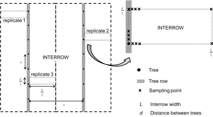
In the agroforestry plots, the soil was sampled taking into account the spatial heterogeneity introduced by the trees and tree rows. This was done by defining an elementary sampling pattern that allowed addressing all situations: more or less close to a tree, in the tree row or in the cropped interrow. The sampling pattern included 12 sampling points along three transects (Figure 1):
5
- four points in a tree row: at 1, 2 and 3 m from a tree, then at the half-distance between two trees;
- four points perpendicularly to a tree row, in front of a tree: at the edge of the grass cover, then 1 and 2 m away, and finally, in the middle of the interrow;
- four points perpendicularly to a tree row but at the half-distance between two trees: at the edge of the grass cover, then 1 and 2 m away, and finally, in the middle of the interrow. This sampling pattern was replicated three times in each agroforestry plot. The sampling pattern in the agricultural plots (without trees), also replicated three times, was simpler and included four points forming a rectangle; the short side was 6 m and the long side was half the interrow width. In each field, 144 soil samples were collected for the conventional determination of SOC stock, representing a total of 288 samples for both fields.
Figure 1. Soil sampling scheme in the agroforestry plots.
At each sampling point, the sample SOC stock (SSOC, in gC kg-1 soil) was determined conventionally at 0-10, 10-20 and 20-30 cm depth. This was done by measuring soil bulk density (Db, in kg dm-3) using a 0.5 L beveled cylinder (≈ 9 cm high) and by determining SOC
concentration (gC kg-1 soil) on the same sample (Blake, 1965). The samples were air-dried and sieved to pass through a 2 mm mesh. Crop residues, root material and stones and gravels > 2 mm were removed during sieving since coarse particles are considered to not contain SOC, and were weighed. The Db was calculated as the ratio of the mass of dry fine earth
Tree Tree row Sampling point
L Interrow width
d Distance between trees
2 L 2 d INTERROW replicate 1 replicate 2 replicate 3 INTERROW 2 d 2 L d L
6
(< 2 mm) to the cylinder volume (Throop et al., 2012). The mass of dry fine earth was determined from aliquots that were oven-dried at 105°C for 48 h and weighed. The determination of SOC concentration was carried out on finely ground (< 0.2 mm) and oven-dried (40°C) aliquots of fine earth by dry combustion using an Elemental Analyzer (CHN Fisons/Carlo Erba NA 2000, Milan, Italy). In the absence of carbonates, which was checked using chlorhydric acid, all carbon was assumed to be organic. Laboratory replication was not achieved because this would have been expensive, and because preliminary tests showed that the standard deviation of the conventional SOC analysis was small (< 5% of the mean). The SOC concentration was expressed as a proportion of fine earth dried at 105°C and then multiplied by Db to determine SSOC. Four conventionally determined variables were
considered for VNIRS prediction: SOC concentration in the fine earth (< 2 mm; SOCfe), SOC
concentration as a proportion of total soil (including coarse particles; SOCts), Db and SOC
stock (SSOC).
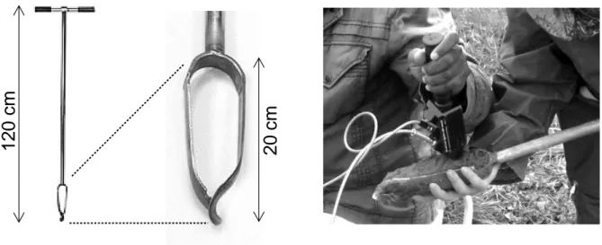
Figure 2. Manual auger and scan of a manual auger core.
2.3. Spectrum acquisition and analysis
Reflectance spectra in the visible and near infrared range were collected in the field, on the outer side of cores collected using a manual auger (Figure 2). Indeed, Gras et al. (2014) demonstrated this was an appropriate procedure for collecting soil VNIR spectra in the field. Before cylinder sampling (cf. 2.2), soil auger cores were sampled at three points at about 0.4 m around each future cylinder sampling location. On each core, one spectrum was acquired at 3 and at 7 cm for the 0-10 cm layer, at 13 and at 17 cm for the 10-20 cm layer, and at 23 and at 27 cm for the 20-30 cm layer. The six spectra acquired per 10-cm soil layer and
1
2
0
cm
2
0
cm
7
corresponding to a cylinder sample were then averaged. Diffuse reflectance was measured from 350 to 2500 nm at 1 nm interval using a portable spectrophotometer LabSpec 2500 (ASD, Boulder, CO, USA). In this device, light is delivered to the sample by a contact probe (about 3 cm² area), which then collects the reflected signal and transmits it to the spectrometer. After every spectral acquisition, the window of the contact probe was cleaned with lens paper and ethanol. The white reference standard, with zero absorbance, was a disc made of Spectralon (compressed polytetrafluoroethylene powder) and its reflectance was measured every 12 acquisitions. Each reflectance spectrum provided by the spectrometer resulted from the averaging of 32 co-added scans. Spectral data were recorded as absorbance, which is the logarithm of the inverse of reflectance [log(1/reflectance)].
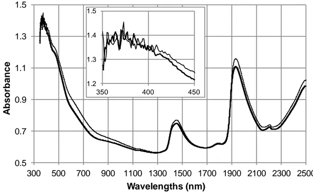
Figure 3. Absorbance spectra of two example samples, with details on the 350-450 nm
region.
Spectrum analysis consisted in fitting the VNIR spectra to the conventionally determined variables (SOCfe, SOCts, Db and SSOC). Data analysis was conducted using the WinISI 4
software (Foss NIRSystems / Tecator Infrasoft International, State College, PA, USA). This was done testing three wavelength ranges, 350-2500, 400-2500 and 450-2500 nm, because spectrum lower end was often noisy (cf. Figure 3). Firstly, VNIR spectra were pre-processed, which consists of mathematically transforming the signal in order to amplify its useful parts (e.g. relating to chemical properties) and reduce irrelevant information (e.g. resulting from light scattering). Seven pre-processing methods were tested: none (no transformation),
0.5 0.7 0.9 1.1 1.3 1.5 300 500 700 900 1100 1300 1500 1700 1900 2100 2300 2500 A b s o rb a n c e Wavelengths (nm) 1.2 1.3 1.4 1.5 350 400 450
8
standard normal variate (SNV) transformation, de-trending (D), SNVD (i.e. both SNV and D) and standard, inverse or weighted multiplicative scatter correction (MSC, IMSC and WMSC, respectively; Geladi et al., 1985; Barnes et al., 1989). These seven spectral transformations were combined, or not, with first derivation. Derivation aims at reducing baseline variation and enhancing spectral features, and was calculated over a , 1 or 20-point gap, with 5-point smoothing, in order to reduce signal random noise (Bertrand, 2000). This led to five combinations: no derivatives with 1- or 5-point smoothing (denoted as 0 0 1 and 0 0 5, respectively); first derivatives with 5-, 15- or 20-point gap and 5-point smoothing (1 5 5, 1 15 5 and 1 20 5, respectively). On the whole, the seven transformations and five derivation procedures tested resulted in 35 pre-processing methods.
A principal component analysis (PCA) was then carried out to calculate the Mahalanobis distance, H (Mark and Tunnel, 1985). Three samples, which had atypical spectra (H > 3), were considered spectral outliers because of a probable problem during spectrum acquisition. Two cases were tested: removing or not these three samples, for each pre-processing method in the three wavelength ranges. The set made of 288 samples (or 285 when removing the three spectral outliers) was then divided into a calibration subset, including 200 samples, and a remaining validation subset, which included 88 (or 85) samples. The calibration subset was selected by the software to include the most spectrally representative samples of the set (by selecting a sample from a neighbouring pair of samples in the principal component space). Then, modified partial least squares (PLS) regression was used to derive calibration models from spectra and conventionally determined variables (Shenk and Westerhaus, 1991). The PLS regression is a linear multivariate regression procedure useful to reduce a complex spectral matrix into a few orthogonal components, or terms, and has often been considered an appropriate statistical method for studying soil organic properties (Reeves et al., 2002; Brunet et al., 2007; Nocita et al., 2013). The modification of the PLS proposed by Shenk and Westerhaus (1991) consisted of scaling the conventional data and the reflectance data at each wavelength to have a standard deviation of 1.0 before each PLS term. Cross-validation was performed on the calibration subset to determine the optimal number of terms to be included in the prediction model. In the present case, the calibration subset was divided into six groups: five used to develop the model and one to test it, and the procedure was performed six times to use all samples for both model development and prediction. The six groups were selected cyclically (i.e. the first group included the 1st, 7th, 13th sample, etc.; the second group included the 2nd, 8th, 14th sample, etc.) after the samples had been ranked in alphabetical order, which reflected their spatial proximity. The residuals of the six predictions were pooled to calculate
9
the standard error of cross-validation between predicted and measured values (SECV), according to equation (1):
SECV = 𝑁𝑐𝑎𝑙1 (ŷ𝑖−𝑦𝑖)²
𝑁𝑐𝑎𝑙 −1 , (1)
where yi is the conventionally determined value for sample i, ŷi the value predicted by the
model for sample i, and Ncal the size of the calibration subset (Mark and Workman, 2003).
Two cases were studied: calibration outliers (i.e. samples with residual greater than 2.5 times SECV) were either removed, then another cross-validation was performed, the procedure being carried out twice, and all remaining calibration samples were used to calculate the final model; or calibration outliers were not removed. The number of calibration outliers ranged from 2 to 17, averaged 9, and depended on the variable considered, on the wavelength range, on the possible removal of spectral outliers, and on the pre-processing method. The calibration performance was assessed using the coefficient of determination (R²cv) and the
ratio of standard deviation of the calibration subset to SECV (denoted as RPDcv). Then, the
prediction accuracy of the calibration model was tested on the validation subset. The performance parameters for validation were the coefficient of determination (R²val) and the
standard error of prediction corrected for bias (SEPc, Eq. 2 and 3):
SEPc = (ŷ𝑖−𝑦𝑖−𝑏𝑖𝑎𝑠 )² 𝑁𝑣𝑎𝑙 1 𝑁𝑣𝑎𝑙 , (2) and bias = 𝑁𝑣𝑎𝑙1 (ŷ𝑖−𝑦𝑖) 𝑁𝑣𝑎𝑙 , (3)
where Nval is the size of the validation subset. The ratio of standard deviation of the validation
subset to SEPc (denoted as RPDval) was also considered. The significance of differences in
model accuracy according to the wavelength range, pre-processing method or possible removal of outliers was not assessed.
3. Results
3.1. Conventional data
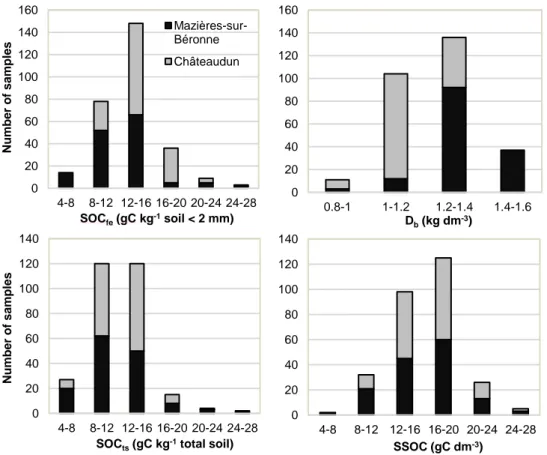
Reference data resulting from conventional determinations are presented in Table 1, with frequency histograms in Figure 4. The studied population displayed wide ranges of SOCfe (the
ratio of maximum to minimum was 4.6), SOCts (ratio 4.4) and SSOC (ratio 3.5), but Db varied
much less (ratio 1.8). Figure 4 shows that samples tended to have higher SOC concentration and lower Db in Châteaudun than in Mazières-sur-Béronne; as a result, SSOC distributions
10
were similar at both sites. There were close correlations between SOCfe and SOCts
(R² = 0.94), and to a lesser extent between SSOC and SOCts (R² = 0.88) or SOCfe (R² = 0.80),
but no correlation was found between SSOC and Db (R² = 0.04).
Table 1. Conventional determination of SOC concentration in the fine earth (< 2 mm; SOCfe)
and in the total soil (SOCts), of bulk density (Db) and of SOC stock (SSOC) for the total set
(288 samples): minimum, maximum, mean and standard deviation (SD).
Soil property Min Max Mean SD
SOCfe (gC kg-1 fine earth, i.e. soil < 2 mm) 5.7 26.3 13.3 3.4
SOCts (gC kg-1 total soil) 5.5 24.2 12.0 3.0
Db (kg dm-3) 0.85 1.56 1.24 0.13
SSOC (gC dm-3) 7.9 27.7 16.2 3.3
Figure 4. Frequency histograms of conventional data: SOC concentration in the fine earth
(< 2 mm; SOCfe) and in the total soil (SOCts), bulk density (Db), and SOC stock (SSOC). 0 20 40 60 80 100 120 140 160 4-8 8-12 12-16 16-20 20-24 24-28 N umbe r of sa mpl es SOCfe(gC kg-1soil < 2 mm) Mazières-sur-Béronne Châteaudun 0 20 40 60 80 100 120 140 4-8 8-12 12-16 16-20 20-24 24-28 N umbe r of sa mpl es
SOCts(gC kg-1total soil)
0 20 40 60 80 100 120 140 160 0.8-1 1-1.2 1.2-1.4 1.4-1.6 Db(kg dm-3) 0 20 40 60 80 100 120 140 4-8 8-12 12-16 16-20 20-24 24-28 SSOC (gC dm-3)
11 3.2. Prediction models
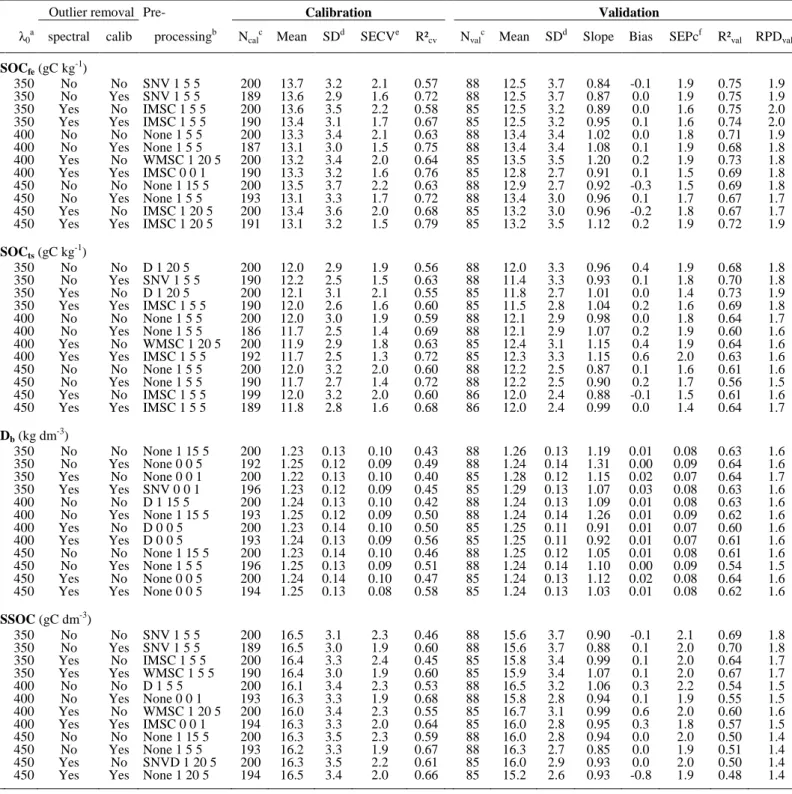
The Table 2 presents the calibration and validation results achieved with the most appropriate pre-processing method (in terms of RPDval) for different spectral ranges (350-, 400- or
450-2500 nm) and with possible removal of the spectral and/or calibration outliers. The spectra of two example samples presented in Figure 3 show their noisy lower end. Nevertheless, better predictions were most often achieved with the complete wavelength range (350-2500 nm) than with 400-2500 nm, and to a greater extent, 450-2500 nm, especially for SSOC. Removing or retaining the spectral and/or calibration outliers did not have much effect on the prediction accuracy. In average, removing the three spectral outliers tended to slightly improve the validation results for SOCfe, SOCts and Db (RPDval increased slightly), but not for
SSOC. In contrast, removing the calibration outliers tended to slightly degrade the validation results for SOCts and Db, but not for SOCfe and SSOC. Removing both the spectral and
calibration outliers also tended to slightly degrade the validation results for SOCfe, SOCts and
Db, but not for SSOC. The most appropriate pre-processing method depended on the
procedure, especially the possible removal of spectral outlier. When the spectral outliers were retained, None 1 5 5, and SNV 1 5 5 to a lesser extent, often yielded the best validations (RPDval), or among the best, for SOCfe, SOCts and SSOC, while None 1 15 5 did the same for
Db. When the spectral outliers were removed, IMSC 1 5 5, and WMSC 1 20 5 to a lesser
extent, often yielded the best validations, or among the best, for SOCfe, SOCts and SSOC,
while None 0 0 1 did the same for Db.
Whatever the variable, RPDval hardly reached 2, which has been considered a threshold for
accurate NIRS prediction of soil properties (Chang et al., 2001). Nevertheless, in optimal conditions (wavelength range, pre-processing method and outlier management), RPDval of at
least 1.6 could be achieved for the four variables, which has been considered acceptable for NIRS prediction of soil properties (Dunn et al., 2002). Prediction accuracy tended to decrease slightly from SOCfe to SOCts, then to SSOC and finally Db. Bias was low in general. The
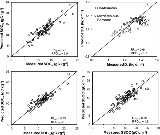
Figure 5 shows scatter plots that compare predicted values obtained with the most accurate models and conventionally determined values, for the validation set and for each soil property. Samples from both sites were well discriminated for Db, but not for the other
variables. Separate site calibrations could have been built for Db, but actually the main
objective of the study was to predict SSOC and Db prediction was a by-product, thus no
attempt was made to build prediction models of Db per site.
The regression coefficients of the VNIRS prediction models were examined in order to identify similarities and differences between the regions that contributed heavily to the
12
Table 2. Calibration and validation results using the pre-processing methods that yielded the
best validation, for each studied wavelength range (350-, 400- and 450-2500 nm), with possible removal of spectral and/or calibration outliers.
Outlier removal Pre- Calibration Validation
λ0
a
spectral calib processingb Ncal
c
Mean SDd SECVe R²cv Nval
c
Mean SDd Slope Bias SEPcf R²val RPDval
g
SOCfe (gC kg-1)
350 No No SNV 1 5 5 200 13.7 3.2 2.1 0.57 88 12.5 3.7 0.84 -0.1 1.9 0.75 1.9
350 No Yes SNV 1 5 5 189 13.6 2.9 1.6 0.72 88 12.5 3.7 0.87 0.0 1.9 0.75 1.9
350 Yes No IMSC 1 5 5 200 13.6 3.5 2.2 0.58 85 12.5 3.2 0.89 0.0 1.6 0.75 2.0
350 Yes Yes IMSC 1 5 5 190 13.4 3.1 1.7 0.67 85 12.5 3.2 0.95 0.1 1.6 0.74 2.0
400 No No None 1 5 5 200 13.3 3.4 2.1 0.63 88 13.4 3.4 1.02 0.0 1.8 0.71 1.9
400 No Yes None 1 5 5 187 13.1 3.0 1.5 0.75 88 13.4 3.4 1.08 0.1 1.9 0.68 1.8
400 Yes No WMSC 1 20 5 200 13.2 3.4 2.0 0.64 85 13.5 3.5 1.20 0.2 1.9 0.73 1.8
400 Yes Yes IMSC 0 0 1 190 13.3 3.2 1.6 0.76 85 12.8 2.7 0.91 0.1 1.5 0.69 1.8
450 No No None 1 15 5 200 13.5 3.7 2.2 0.63 88 12.9 2.7 0.92 -0.3 1.5 0.69 1.8
450 No Yes None 1 5 5 193 13.1 3.3 1.7 0.72 88 13.4 3.0 0.96 0.1 1.7 0.67 1.7
450 Yes No IMSC 1 20 5 200 13.4 3.6 2.0 0.68 85 13.2 3.0 0.96 -0.2 1.8 0.67 1.7
450 Yes Yes IMSC 1 20 5 191 13.1 3.2 1.5 0.79 85 13.2 3.5 1.12 0.2 1.9 0.72 1.9
SOCts (gC kg-1)
350 No No D 1 20 5 200 12.0 2.9 1.9 0.56 88 12.0 3.3 0.96 0.4 1.9 0.68 1.8
350 No Yes SNV 1 5 5 190 12.2 2.5 1.5 0.63 88 11.4 3.3 0.93 0.1 1.8 0.70 1.8
350 Yes No D 1 20 5 200 12.1 3.1 2.1 0.55 85 11.8 2.7 1.01 0.0 1.4 0.73 1.9
350 Yes Yes IMSC 1 5 5 190 12.0 2.6 1.6 0.60 85 11.5 2.8 1.04 0.2 1.6 0.69 1.8
400 No No None 1 5 5 200 12.0 3.0 1.9 0.59 88 12.1 2.9 0.98 0.0 1.8 0.64 1.7
400 No Yes None 1 5 5 186 11.7 2.5 1.4 0.69 88 12.1 2.9 1.07 0.2 1.9 0.60 1.6
400 Yes No WMSC 1 20 5 200 11.9 2.9 1.8 0.63 85 12.4 3.1 1.15 0.4 1.9 0.64 1.6
400 Yes Yes IMSC 1 5 5 192 11.7 2.5 1.3 0.72 85 12.3 3.3 1.15 0.6 2.0 0.63 1.6
450 No No None 1 5 5 200 12.0 3.2 2.0 0.60 88 12.2 2.5 0.87 0.1 1.6 0.61 1.6
450 No Yes None 1 5 5 190 11.7 2.7 1.4 0.72 88 12.2 2.5 0.90 0.2 1.7 0.56 1.5
450 Yes No IMSC 1 5 5 199 12.0 3.2 2.0 0.60 86 12.0 2.4 0.88 -0.1 1.5 0.61 1.6
450 Yes Yes IMSC 1 5 5 189 11.8 2.8 1.6 0.68 86 12.0 2.4 0.99 0.0 1.4 0.64 1.7
Db (kg dm-3) 350 No No None 1 15 5 200 1.23 0.13 0.10 0.43 88 1.26 0.13 1.19 0.01 0.08 0.63 1.6 350 No Yes None 0 0 5 192 1.25 0.12 0.09 0.49 88 1.24 0.14 1.31 0.00 0.09 0.64 1.6 350 Yes No None 0 0 1 200 1.22 0.13 0.10 0.40 85 1.28 0.12 1.15 0.02 0.07 0.64 1.7 350 Yes Yes SNV 0 0 1 196 1.23 0.12 0.09 0.45 85 1.29 0.13 1.07 0.03 0.08 0.63 1.6 400 No No D 1 15 5 200 1.24 0.13 0.10 0.42 88 1.24 0.13 1.09 0.01 0.08 0.63 1.6 400 No Yes None 1 15 5 193 1.25 0.12 0.09 0.50 88 1.24 0.14 1.26 0.01 0.09 0.62 1.6 400 Yes No D 0 0 5 200 1.23 0.14 0.10 0.50 85 1.25 0.11 0.91 0.01 0.07 0.60 1.6 400 Yes Yes D 0 0 5 193 1.24 0.13 0.09 0.56 85 1.25 0.11 0.92 0.01 0.07 0.61 1.6 450 No No None 1 15 5 200 1.23 0.14 0.10 0.46 88 1.25 0.12 1.05 0.01 0.08 0.61 1.6 450 No Yes None 1 5 5 196 1.25 0.13 0.09 0.51 88 1.24 0.14 1.10 0.00 0.09 0.54 1.5 450 Yes No None 0 0 5 200 1.24 0.14 0.10 0.47 85 1.24 0.13 1.12 0.02 0.08 0.64 1.6
450 Yes Yes None 0 0 5 194 1.25 0.13 0.08 0.58 85 1.24 0.13 1.03 0.01 0.08 0.62 1.6
SSOC (gC dm-3) 350 No No SNV 1 5 5 200 16.5 3.1 2.3 0.46 88 15.6 3.7 0.90 -0.1 2.1 0.69 1.8 350 No Yes SNV 1 5 5 189 16.5 3.0 1.9 0.60 88 15.6 3.7 0.88 0.1 2.0 0.70 1.8 350 Yes No IMSC 1 5 5 200 16.4 3.3 2.4 0.45 85 15.8 3.4 0.99 0.1 2.0 0.64 1.7 350 Yes Yes WMSC 1 5 5 190 16.4 3.0 1.9 0.60 85 15.9 3.4 1.07 0.1 2.0 0.67 1.7 400 No No D 1 5 5 200 16.1 3.4 2.3 0.53 88 16.5 3.2 1.06 0.3 2.2 0.54 1.5 400 No Yes None 0 0 1 193 16.3 3.3 1.9 0.68 88 15.8 2.8 0.94 0.1 1.9 0.55 1.5 400 Yes No WMSC 1 20 5 200 16.0 3.4 2.3 0.55 85 16.7 3.1 0.99 0.6 2.0 0.60 1.6
400 Yes Yes IMSC 0 0 1 194 16.3 3.3 2.0 0.64 85 16.0 2.8 0.95 0.3 1.8 0.57 1.5
450 No No None 1 15 5 200 16.3 3.5 2.3 0.59 88 16.0 2.8 0.94 0.0 2.0 0.50 1.4
450 No Yes None 1 5 5 193 16.2 3.3 1.9 0.67 88 16.3 2.7 0.85 0.0 1.9 0.51 1.4
450 Yes No SNVD 1 20 5 200 16.3 3.5 2.2 0.61 85 16.0 2.9 0.93 0.0 2.0 0.50 1.4
450 Yes Yes None 1 20 5 194 16.5 3.4 2.0 0.66 85 15.2 2.6 0.93 -0.8 1.9 0.48 1.4
a
Lower end of the wavelength range considered (nm).
b
See section 2.3 for the pre-processing methods.
c
Size of the calibration and validation subset, respectively.
d
Standard deviation of the calibration and validation subset, respectively.
e
Standard error of cross-validation (in the unit of the variable).
f
Standard error of prediction corrected for bias (in the unit of the variable).
g
13
Figure 5. Comparison between conventionally determined and VNIRS predicted values of
SOCfe (fine earth), SOCts (total soil), Db and SOC stock (SSOC) for validation samples
(predictions made using the whole 350-2500 nm range; distinction between both sites was hardly possible except for Db).
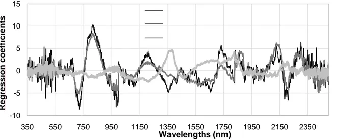
prediction of the different variables. This was done for models built with raw absorbance spectra (denoted None 0 0 1), which are easier to interpret than those using pre-processed spectra, especially first derivatized spectra (though they often yielded less accurate predictions). Indeed, it is not trivial to interpret the regions where absorbance varies the most (i.e. peaks of first derivatized spectra). The comparison of regression coefficients between the SOCfe and SOCts models did not reveal any noticeable difference (data not shown). Figure 6
presents the regression coefficients for SOCfe, SSOC and Db. It shows that several spectral
regions that contributed heavily to the predictions were similar for SOCfe and SSOC (e.g.
around 815 and 1200 nm), but that others were not (e.g. the respective contributions of the
0 5 10 15 20 25 0 5 10 15 20 25 P re d ic te d S O Cfe (g C k g -1) Measured SOCfe(gC kg-1) 1:1 R²val= 0.75 RPDval= 2.0 0.8 1.0 1.2 1.4 1.6 0.8 1 1.2 1.4 1.6 P re d ic te d Db (k g d m -3) Measured Db(kg dm-3) Châteaudun Mazières-sur-Béronne 1:1 R²val= 0.64 RPDval= 1.7 0 5 10 15 20 25 0 5 10 15 20 25 P re d ic te d S O Cts (gC kg -1) Measured SOCts(gC kg-1) 1:1 R²val= 0.73 RPDval= 1.9 0 5 10 15 20 25 30 0 5 10 15 20 25 30 P re d ic te d S S O C ( gC dm -3) Measured SSOC (gC dm-3) 1:1 R²val= 0.70 RPDval= 1.8
14
regions around 1350, 1650, 1700, 1870, 2150 and 2190 nm differed for SOCfe and SSOC);
thus the prediction of SSOC was not indirect through the prediction of SOCfe. The prediction
of Db involved different heavily contributing regions (e.g. 1360-1680 nm). Whatever the
variable, the regions below 550 nm and beyond 2320 nm seemed poorly informative.
4. Discussion
According to Chang et al. (2001) and Dunn et al. (2002), NIRS predictions of soil properties can be considered accurate when RPD ≥ 2.0, acceptable when 1.6 ≤ RPD < 2.0, and poor when RPD < 1.6. According to this classification, an accurate model of SOCfe prediction was
achieved (RPDval = 2.0; SEPc = 1.6 gC kg-1 soil < 2 mm), but this was less accurate than in
some previous literature studies. Indeed, Gras et al. (2014) reported good VNIRS prediction of soil organic matter concentration, with RPDcv = 2.8 and SECV = 2.4 gC kg-1. These results
were also achieved using field VNIRS applied on cores collected with a manual auger, but in cross-validation, which results in less robust models than external validation. Moreover, Gras et al. (2014) studied a soil population collected at one depth layer (0-20 cm), but more diverse geographically: it originated from six cropped fields located over France, and the coefficient of variation (CV, i.e. ratio of standard deviation to mean) for SOCfe was 44% (vs. 26% here).
Furthermore, these authors carried out conventional analysis and spectrum acquisition on the same samples, which was not the case here; indeed, this would have required scanning the cylinder samples, whereas the study aimed at predicting SOC stock without cylinder sampling (except for calibration). In addition, the study of Gras et al. (2014) was conducted in winter and the samples were rather constantly moist, while the present study was conducted in spring and some superficial samples were rather dry. Dry soil conditions have been reported by several authors as being less favourable than moist conditions for VNIRS predictions of SOC concentration, as long as moisture content is not too heterogeneous between samples (Stenberg, 2010; Nocita et al., 2013). Finally, though rather different experimental conditions, the accuracy of VNIRS predictions of SOCfe could be considered somewhat similar in the
present study and in that of Gras et al. (2014). Morgan et al. (2009) studied VNIR spectra acquired on moist cores in six fields from two Texas counties and achieved poor results in external validation for SOCfe (RPDval = 1.5 and SEPc = 5.3 gC kg-1). This might firstly be
attributed to the wide diversity of the soils they studied (five soil orders, texture varying from clay to sand, CV = 106% for SOCfe), which is a source of inaccuracy for (V)NIRS predictions
(Brunet et al., 2007). Furthermore, Morgan et al. (2009) used reflectance data for making predictions, and it is possible that absorbance data would have yielded better predictions.
15
Moreover, Morgan et al. (2009) grouped the samples by profile and selected the calibration and validation profiles at random, which improved the robustness of prediction models but resulted in less accurate validation than building calibration on the most representative samples, as was done in the present study. Stevens et al. (2008) also used field VNIRS to predict SOCfe at a regional scale (50 km² area) and achieved poor external validation
(RPDval = 1.2; SEPc = 7.0 gC kg-1), possibly due to the fact that they used a spectroradiometer
to scan a spot size of 0.45 m from 1 m height, while reference analyses were made on a much smaller sample collected to a depth of 5 cm. In addition, the calibration and validation sets were randomly selected, but apparently sample diversity was limited though regional scale was addressed (CV = 20% for SOCfe).
Figure 6. Regression coefficients of the VNIRS prediction models of SOCfe, SSOC (SOC
stock) and Db built using raw absorbance spectra (None 0 0 1).
Field VNIRS predictions of SOCts and Db have not been reported in the literature to date.
Here SOCts was slightly less accurately predicted than SOCfe (RPDval = 1.9;
SEPc = 1.4 gC kg-1 total soil), probably due to error propagation, as the conventional determination of SOCts required weighting SOCfe by the proportion of fine earth in the total
soil. The VNIRS prediction of Db was acceptable but not accurate (RPDval = 1.7;
SEPc = 0.07 g cm-3) due to the fact that auger sampling resulted in some torsion of the sample, which thus had its structure and porosity altered. Moreover, Db was less variable than
the other studied variables (CV = 10% vs. 20-25%), which did not help prediction. Moreira et al. (2009) tried to predict Db using laboratory NIRS on 2 mm sieved air dried samples but
achieved poor results (RPDval = 1.2; SEPc = 0.12 g cm-3), due to important loss of information
-10 -5 0 5 10 15 350 550 750 950 1150 1350 1550 1750 1950 2150 2350 R eg ression co eff icients Wavelengths (nm)
16
on bulk density resulting from sample sieving. Minasny et al. (2008) similarly failed to predict Db from mid-infrared spectra of dried, 0.2 mm ground samples (RPDval = 1.2;
SEP = 0.09 g cm-3). Using VNIR spectra of dried, 0.2 mm ground samples, Askari et al. (2015) predicted Db with validation results comparable to ours for arable soils (RPDval = 1.7;
SEPc = 0.06 g cm-3), and even achieved good prediction of Db at 2 mm particle size
(calculated after separating gravel > 2 mm) for grassland soils (RPDval = 2.1;
SEPc = 0.06 g cm-3). For a diverse set of soils (sandy to clayey texture) studied at 10-20 cm depth, Al-Asadi and Mouazen (2014) achieved accurate prediction of Db as the ratio of
volumetric moisture content, predicted using frequency domain reflectometry in the field, and gravimetric moisture content, predicted using VNIRS on fresh samples, when calibrations were based on artificial neural network analysis (RPDval = 2.3; SEP = 0.10 g cm-3); by
contrast, they got poor predictions when using PLS regressions (RPDval = 1.2-1.4;
SEP = 0.16-0.19 g cm-3).
The VNIRS prediction of SSOC was less accurate than those of SOCfe and SOCts but was
acceptable, especially when considering that the reference method is tedious (cylinder sampling): RPDval = 1.8 and SEPc = 2.0 gC dm-3, representing 13% of the mean (with the
most appropriate pre-processing method). In addition, as for SOC concentration predictions, the bias was low, and large values were not particularly associated with underpredictions or large residues. This suggested that VNIRS prediction of SSOC was relevant and that prediction errors, as for SOC concentration prediction, could be attributed, at last partly, to the fact that spectrum acquisition and conventional analyses were not carried out on the same samples. This point could be addressed by studying the variations of conventionally determined properties over short distances (0.4 m). Above all, it could be possible to limit this issue by performing conventional SOC concentration analysis on the auger core used to get the VNIR spectrum, rather than on the cylinder core used for determining Db. As SSOC
variations depended (and generally depend) much more on SOC concentration variations than on Db variations, this would limit the discrepancy between soil materials used for
conventional determination and VNIRS prediction of SSOC. As a consequence, this would improve the calibration of SOC concentration and SSOC. However, characterizing Db and
SOC concentration on different samples would result in less reliable conventional determination of SSOC, which might be an issue. It is a troublesome fact that the most appropriate procedure for conventional SSOC determination seemed to not be the most appropriate for SSOC calibration (as long as cylinder samples were not scanned, which was a requirement). It is also troublesome that the conventional determination of SOC concentration
17
on manual auger cores would improve SSOC calibration based on less reliable conventional SSOC determination. Furthermore, replication of conventional SSOC determination was not achieved in the present study, and the uncertainty on SSOC was attributed to VNIRS prediction (as part of the standard error). Some error propagation could also be possible in the conventional determination of SSOC, which was not measured but calculated as the product of SOCfe and Db. Very few literature papers have addressed VNIRS prediction of SSOC in the
field. In an unpublished paper, Roudier et al. (2012) reported such prediction from spectra acquired on soil cores collected using a hydraulic coring truck, in one 68.5 ha field, with fairly good results (RPDval = 2.2; SEPc was not mentioned). In that case, hydraulic core sampling
resulted in less soil disturbance than in the present study (manual auger sampling); in addition, VNIRS and conventional analyses were carried out on the same sample, which, along with the fact that one site only was considered, could explain better results.
The accuracy of VNIRS prediction models was higher when using the whole wavelength range (350-2500 nm) than when the lower end was removed (400- or 450-2500 nm), for every studied variable. A possible explanation is that noise did not affect many wavelengths in the 350-450 nm range, and that this could be managed by the PLS regression. By contrast, removing a 50 or 100 nm region represented a loss of information, which resulted in degraded prediction models. Better validation results after the removal of the three spectral outliers could be explained by higher overall sample set homogeneity. Indeed, when such samples are retained, the prediction models have to take account, to some extent, of their atypicality, and as a consequence, are less adapted to the more typical other samples. Here this effect was slight in general because there were only three spectral outliers, and their atypicality was limited (H < 5). Worse validation results after the removal of the calibration outliers could be explained by higher calibration subset homogeneity, which resulted in lower model robustness. Indeed, except when large residues are caused by errors in the conventional or spectral data, removing calibration outliers renders the calibration subset more homogeneous, thus less representative of the validation subset. In general the effect was slight here because there were few calibration outliers (4% of the calibration subset in average, and 7% at most). As regards spectrum pre-processing, the best results generally required first derivatization, which removes additive effects (e.g. due to baseline shift), and smoothing, with reduces random noise (Bertrand, 2000). When the spectral outliers were deleted, multiplicative scatter corrections, which remove multiplicative effects (e.g. due to particle size; Bertrand, 2000), were also required for improving the prediction of SOC content and stock.
18
The fact that spectral regions that contributed heavily to SOCfe and SSOC predictions were
not similar indicates that SSOC was not predicted indirectly through the prediction of SOCfe
and correlation between SOCfe and SSOC. In addition, correlations between SSOC and SOCfe
or SOCts (R² = 0.80-0.88) were not sufficient to allow the indirect prediction of SSOC
(R²val = 0.70) through the prediction of SOCfe or SOCts (R²val = 0.73-0.75).
The studied sample set did not include soaked soils or dry soils, which might be considered a limit. However, as for every VNIRS study of soils in the field, it is preferable that the soil is not soaked or dry; this is not specific to the prediction of SSOC. Soaked soils are difficult to work on and manipulate, while dry soils have weak cohesion, which weakens the reflectance signal thus is not favourable for predictions (Stenberg, 2010; Nocita et al., 2013; Gras et al., 2014). The rather moist samples studied here could thus be considered representative of the appropriate conditions for field VNIRS on soils.
5. Conclusion and perspectives
This study showed the potential of field VNIRS to predict accurately SOC concentration and acceptably SOC stock from partially disturbed cores sampled using a manual auger, in two agroforestry fields on silty Luvisols. Fine earth SOC concentration was predicted with R²val = 0.75, SEPc = 1.6 gC kg-1 soil < 2 mm, and RPDval = 2.0; and SOC stock with
R²val = 0.70, SEPc = 2.0 gC dm-3, and RPDval = 1.8. Removing spectral and/or calibration
outliers had no clear effect on VNIRS prediction accuracy. By contrast, removing the noisy lower end of the spectra (350-400 or 350-450 nm) caused a deterioration of prediction accuracy.
A part of the prediction error could be attributed to the fact that conventional determinations of SOC concentration and bulk density were carried out on cylinder samples, while spectra were acquired on auger cores collected at three points at 0.4 m around. Determining SOC concentration on the auger core used for spectrum acquisition would probably improve the calibration of SOC concentration and thus of SOC stock, because the variations of SOC stock depended mainly on the variations of SOC concentration (as bulk density varied much less). This work indicates that time- and cost-effective determination of SOC stock from VNIR spectra acquired on manual auger cores could be a valuable solution for tackling the lack of data on SOC stocks.
19 Acknowledgements
This work was supported by the INCA project (In-field spectroscopy for carbon accounting; coord. Véronique Bellon-Maurel and Alexia Gobrecht) of the GESSOL program of the French Ministry of ecology, sustainable development and energy, and was funded by ADEME (Agence de l'environnement et de la maîtrise de l'énergie, which is a French government agency dedicated to environmental protection and energy management; contract ADEME – University of Sydney – CEMAGREF/IRSTEA - INRA - IRD N°1060C0093). The authors are very grateful to the farmers, Mr. Thierry Franchet (Châteaudun) and Mr. Pierre Bernard (Mazières-sur-Béronne), for authorizing soil sampling in their fields. The authors also thank Agroof, an engineering office specialized in agroforestry systems, for its help in the logistics. The help of Clément Renoir during sample preparation is also acknowledged.
References
Al-Asadi, R.A., Mouazen, A.M., 2014. Combining frequency domain reflectometry and visible and near infrared spectroscopy for assessment of soil bulk density. Soil Till. Res. 135, 60–70. doi: 10.1016/j.still.2013.09.002.
Askari, M.S., O'Rourke, S.M., Holden, N.M., 2015. Evaluation of soil quality for agricultural production using visible–near-infrared spectroscopy. Geoderma 243–244, 80-91. doi: 10.1016/j.geoderma.2014.12.012.
Barnes, R.J., Dhanoa, M.S., Lister, S.J., 1989. Standard normal variate transformation and de-trending of near-infrared diffuse reflectance spectra. Appl. Spectrosc. 43, 772–777. doi: 10.1366/0003702894202201.
Barthès, B.G., Brunet, D., Ferrer, H., Chotte, J.L., Feller, C., 2006. Determination of total carbon and nitrogen content in a range of tropical soils using near infrared spectroscopy: influence of replication and sample grinding and drying. J. Near Infrared Spectrosc. 14, 341–348. doi: 10.1255/jnirs.686. Bertrand, D., 2000. Prétraitement des données spectrales, in: Bertrand, D., Dufour, E. (Eds.), La
Spectroscopie Infrarouge et ses Applications Analytiques, 2nd ed. Tec & Doc, Paris, pp. 351–393. Blake, G.L., 1965. Bulk density, in: Black, C.A. (Ed.), Methods of Soil Analysis. Part 1. Am. Soc.
Agron. Monograph 9, Madison, WI, pp. 374–390. doi: 10.2134/agronmonogr9.1.c30.
Brunet, D., Barthès, B.G., Chotte, J.L., Feller, C., 2007. Determination of carbon and nitrogen contents in Alfisols, Oxisols and Ultisols from Africa and Brazil using NIRS analysis: effects of sample grinding and set heterogeneity. Geoderma 139, 106–117. doi: 10.1016/j.geoderma.2007.01.007.
Burns, D.A., Ciurczak, E.W. (Eds.), 2008. Handbook of Near-Infrared Analysis, 3rd ed. CRC Press, Boca Raton, FL.
Chang, C.W., Laird, D.A., Mausbach, M.J., Hurburgh, C.R.J., 2001. Near-infrared reflectance spectroscopy —Principal components regression analyses of soil properties. Soil Sci. Soc. Am. J. 65, 480–490. doi: 10.2136/sssaj2001.652480x.
Dunn, B.W., Beecher, H.G., Batten, G.D., Ciavarella, S., 2002. The potential of near infrared reflectance spectroscopy for soil analysis— a case study from the Riverine Plain of south-eastern Australia. Aust. J. Exp. Agric. 42, 607–614. doi: 10.1071/EA01172.
20
Geladi, P., Mac Dougall, D., Martens, H., 1985. Linearization and scatter-correction for near-infrared reflectance spectra of meat. Appl. Spectrosc. 39, 491–500. doi: 10.1366/0003702854248656.
Gras, J.P., Barthès, B.G., Mahaut, B., Trupin, S., 2014. Best practices for obtaining and processing field visible and near infrared (VNIR) spectra of topsoils. Geoderma 214–215, 126–134. doi: 10.1016/j.geoderma.2013.09.021.
IPCC (International Panel on Climate Change), 2007. Climate Change 2007: Synthesis Report. Contribution of Working Groups I, II and III to the Fourth Assessment Report of the Intergovernmental Panel on Climate Change. Core Writing Team, Pachauri, R.K and Reisinger, A. (Eds.), IPCC, Geneva.
IUSS Working Group WRB (International Union of Soil Sciences, Working Group World Reference Base for Soil Resources), 2006. World Reference Base for Soil Resources 2006. FAO, Rome. Mark, H.L., Tunnell, D., 1985. Qualitative near-infrared reflectance analysis using Mahalanobis
distances. Anal. Chem. 57, 1449–1456. doi: 10.1021/ac00284a061.
Mark, H., Workman, J., 2003. Statistics in Spectroscopy, 2nd ed. Elsevier Science, San Diego, CA. Metz, B., Davidson, O.R., Bosch, P.R., Dave, R., Meyer, L.A. (Eds.), 2007. Contribution of Working
Group III to the Fourth Assessment Report of the Intergovernmental Panel on Climate Change, 2007. Cambridge University Press, Cambridge, UK, and New York.
Minasny, B., McBratney, A.B., Tranter, G., Murphy, B.W., 2008. Using soil knowledge for the evaluation of mid-infrared diffuse reflectance spectroscopy for predicting soil physical and mechanical properties. Eur. J. Soil Sci. 59, 960–971. doi: 10.1111/j.1365-2389.2008.01058.x. Moreira, C.S., Brunet, D., Verneyre, L., Sá, S.M.O., Galdos, M.V., Cerri, C.C., Bernoux, M., 2009.
Near infrared spectroscopy for soil bulk density assessment. Eur. J. Soil Sci. 60, 785–791. doi: 10.1111/j.1365-2389.2009.01170.x.
Morgan, C.L.S., Waiser, T.H., Brown, D.J., Hallmark, C.T., 2009. Simulated in situ characterization of soil organic and inorganic carbon with visible near-infrared diffuse reflectance spectroscopy. Geoderma 151, 249–256. doi: 10.1016/j.geoderma.2009.04.010.
Nocita, M., Stevens, A., Noon, C., van Wesemael, B., 2013. Prediction of soil organic carbon for different levels of soil moisture using Vis-NIR spectroscopy. Geoderma 199, 37–42. doi: 10.1016/j.geoderma.2012.07.020.
Reeves, D.W., 1997. The role of soil organic matter in maintaining soil quality in continuous cropping systems. Soil Till. Res. 43, 131–167. doi: 10.1016/S0167-1987(97)00038-X.
Reeves III, J.B., McCarty, G.W., Mimmo, T., 2002. The potential of diffuse reflectance spectroscopy for the determination of carbon inventories in soils. Environ. Pollut. 116, S277-S284. doi: 10.1016/S0269-7491(01)00259-7.
Roudier, P., Hedley, C., Ross, C., 2012. Farm-scale mapping of soil organic carbon using visible-near
infra-red spectroscopy. Landcare Research, Palmerston, NZ.
http://www.massey.ac.nz/~flrc/workshops/12/Manuscripts/Roudier_2012.pdf [13/01/2015].
Shenk, J.S., Westerhaus, M.O., 1991. Population structuring of near infrared spectra and modified partial least squares regression. Crop Sci. 31, 1548-1555. doi: 10.2135/cropsci1991.0011183X003100060034x.
Stenberg, B., 2010. Effects of soil sample pretreatments and standardised rewetting as interacted with sand classes on Vis-NIR predictions of clay and soil organic carbon. Geoderma 158, 15–22. doi: 10.1016/j.geoderma.2010.04.008.
Stenberg, B., Viscarra Rossel, R.A., Mouazen, A.M., Wetterlind, J., 2010. Visible and near infrared spectroscopy in soil science. Adv. Agron. 107, 163–215. doi: 10.1016/S0065-2113(10)07005-7. Stevens, A., van Wesemael, B., Bartholomeus, H., Rosillon, D., Tychon, B., Ben-Dor, E., 2008.
Laboratory, field and airborne spectroscopy for monitoring organic carbon content in agricultural soils. Geoderma 144, 395–404. doi: 10.1016/j.geoderma.2007.12.009.
21
Stevens, A., Nocita, M., Tóth, G., Montanarella, L., van Wesemael, B., 2013. Prediction of soil organic carbon at the European scale by visible and near infrared reflectance spectroscopy. PLoS ONE 8, e66409. doi: 10.1371/journal.pone.0066409.
Sudduth, K.A., Hummel, J.W., 1991. Evaluation of reflectance methods for soil organic matter sensing. Trans. ASAE 34(4): 1900-1909. doi: 10.13031/2013.31816.
Throop, H.L., Archer, S.R., Monger, H.C., Waltman, S., 2012. When bulk density methods matter: Implications for estimating soil organic carbon pools in rocky soils. J. Arid Environ. 77, 66–71. doi: 10.1016/j.jaridenv.2011.08.020.
Vaughan, D., Malcolm, R.E., 1985. Soil Organic Matter and Biological Activity. Springer, Dordrecht, The Netherlands.