HAL Id: hal-01598285
https://hal.archives-ouvertes.fr/hal-01598285
Submitted on 29 Sep 2017
HAL is a multi-disciplinary open access
archive for the deposit and dissemination of sci-entific research documents, whether they are pub-lished or not. The documents may come from teaching and research institutions in France or abroad, or from public or private research centers.
L’archive ouverte pluridisciplinaire HAL, est destinée au dépôt et à la diffusion de documents scientifiques de niveau recherche, publiés ou non, émanant des établissements d’enseignement et de recherche français ou étrangers, des laboratoires publics ou privés.
Machine learning: A primer
Danilo Bzdok, Martin Krzywinski, Naomi Altman
To cite this version:
Danilo Bzdok, Martin Krzywinski, Naomi Altman. Machine learning: A primer. Nature Methods, Nature Publishing Group, 2017, 14 (12), pp.1119-1120. �hal-01598285�
NATURE METHODS | POINTS OF SIGNIFICANCE Machine learning: A primer
Machine learning extracts general principles from observed examples without explicit instructions.
In previous columns we have discussed several unsupervised learning methods—for example, clustering and principal component analysis— as well as supervised learning methods such as regression and
classification. This month, we begin a series that delves more deeply into algorithms that learn patterns from data to make inferences. This process is called machine learning (ML), a rapidly developing domain closely related to high-dimensional statistics, data mining, pattern recognition, and artificial intelligence. Such methods fall under the broad umbrella of “knowledge discovery”, a computational and quantitative approach to characterize and predict complex phenomena described by many variables.
ML is a strategy to let the data speak for themselves, to the degree possible. Rather than choosing a set of formal assumptions, ML
applies brute-force to fit patterns in the observed data using functions with potentially thousands of weights. Even if there is no a priori model, ML can apply heuristics and numerical optimization to extract patterns from the data. Although ML algorithms typically allow fitting to very complex patterns, data may exhibit salient patterns outside the ML algorithm’s learning capabilities. Due to their adaptive and flexible nature, many ML algorithms perform best when data are abundant [1]. However, increasing data does not necessarily mean that learning improves. ML algorithms are limited by bias in the algorithm and bias in the data, which can produce systematically skewed predictions.
ML is often applied to complicated, poorly understood phenomena in nature [1], such as complex biological systems, climate change,
astronomy, or particle physics. For example, we have little definitive knowledge about the workings of the healthy brain and the
progression and changes associated with neurobiological disease. Mental health researchers studying psychiatric disorders are
struggling to explain the disease mechanisms at the level of genome, epigenetics, thinking and behavior, and life events.
The flexibility of data-guided pattern learning is well suited to address this multitude of possible influences and their complicated relationships. For example, ML algorithms can computationally derive abstract rules to distinguish healthy individuals from affected patients—a process that we cannot expect to be captured by an
explicit equation or hand-picked model. With some a priori
assumptions, ML approaches can identify disease-specific biological aspects that provide potential indicators for accurate diagnosis, treatment, and prognosis in complex diseases.
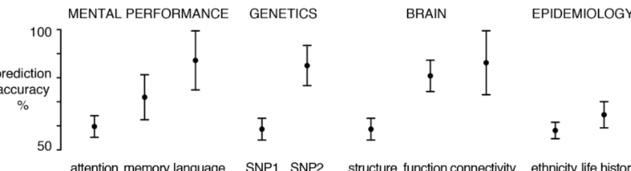
The sensitivity and performance of ML algorithms can be quantified for each potential influence, such as genomic variation, presence of risk variants, brain properties, cognitive performance, and
epidemiological descriptors (Fig. 1). For example, some genetic or neurobiological markers may be more indicative of disease (e.g., genetic mutation or brain connectivity features) and this can provide insight into the mechanisms underlying mental disease. One way to estimate the statistical uncertainty around this and other influences is by bootstrap confidence intervals [3], which estimate how the
prediction would fluctuate in new data from the same population.
Figure 1 | Probing the basis of a psychiatric disorder at multiple levels. Schematic of
how psychological, genetic, neurobiological and epidemiological observations can be used to automatically learn the difference between healthy individuals and affected patients. For each type of measurement (e.g., attention test scores), a learning algorithm is trained on part of the data and subsequently evaluated on remaining test data from independent individuals to obtain prediction performance estimates (50% accuracy corresponds to random guessing). The statistical uncertainty of the prediction accuracies is shown by 95% confidence intervals obtained from bootstrap resampling of data points with replacement.
When applying ML techniques, one question that often arises is “How much data do I need?” To address this, we need to look at some of the fundamental properties of ML.
One of the primary considerations in ML is the n-p ratio, where n is the number of samples and p is the number of variables per
observation. ML is particularly effective in the high-dimensional setting (p >> n) with hundreds or many thousands of variables to be fitted. But, learning algorithms need to tackle the challenges specific to scenarios when p is large—the so-called curse of dimensionality. The danger for overfitting can be counteracted with more samples [4], which allows for a better final algorithmic solution (e.g., higher accuracy in single-patient prediction) and by dimension reduction methods such as PCA.
The complexity of the learning algorithm is critical and should be calibrated with the complexity of the data. The more sophisticated the underlying algorithm, the more data are needed. For instance, a 50th
-order polynomial or a deep neural network algorithm is able to capture very complex trends, but requires abundant data in practice to avoid overfitting. Simple algorithms are often easier to interpret, require less data, and are useful to the extent that complicated interactions between the variables can be neglected. When trained with large data sets, overly simple algorithms that do not overfit can sometimes outperform complex algorithms with the same number of samples [2].
An underlying goal of ML is to approximate the so-called target function, which captures the ground-truth relationship in nature between the input variables (e.g., functional relationships between genes) and an outcome variable (e.g., brain phenotype such as brain or personality disorders). The target function is not known and potentially not knowable. In general, the more complex the target function, the higher the risk for overfitting, so there may still be advantages to choosing a lower-complexity algorithm.
The learning process can be impeded by different sources of
randomness. Stochastic noise is non-identical in different samples drawn from the same population and does therefore not exhibit coherent structure. Such randomness in the data increases the
tendency for overfitting by adapting algorithm weights to noise in the training data. In this case, prediction errors will rise in held-out or new observations. This can be mitigated with larger training sample sizes at the same level of complexity, for example the same number of
adaptive weights.
Typically, ML algorithms cannot achieve perfect accuracy on new data even if the “ground truth” model - the pattern to be uncovered from the data - was known [5,7]. For example, when the relationship between genetic profile and a patient's disease status was known, a learning algorithm that perfectly describes the target function will nevertheless infer wrong outcomes from some new observations. This source of irreducible error is caused by fluctuation in the outcome association with each observation (“label noise”) and is characteristic for each learning problem. It can be quantified using the Bayes error rate (BER), a theoretical quantity capturing algorithm failures that occurred under the condition that the “true” data distribution and the input-output mapping are accessible. In practice, as the amount of data for algorithm training keeps increasing towards the entire population, the maximal performance of an optimal-complexity algorithm predicting new data points converges to the BER.
All these fundamental considerations point to a core insight on ML practice: there is no single right answer to the question how many samples are needed to reach a certain prediction performance.
Moreover, if a relationship between input and output variables exists, we cannot be assured that it can be captured in a given dataset or extracted with a particular learning algorithm (Fig. 2).
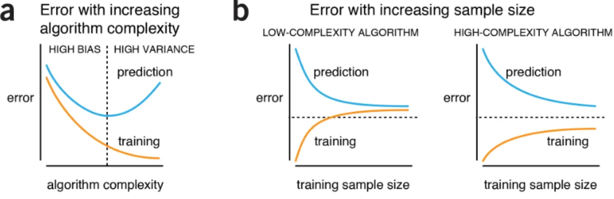
Figure 2 | General behaviors of machine-learning algorithms. (a) When algorithm
complexity is low, both prediction on new data (“prediction error”) and failed model evaluation on the training data (“training error”) are high. In this high-bias regime, prediction is poor because the algorithm has a tendency to underfit structure in the data. As algorithm complexity increases, both errors drop but eventually prediction error rises again. The algorithm enters the high-variance regime, where it starts to overfit. (b) As training sample size increases, for a fixed level of algorithm
complexity, prediction error drops and training error increases. This trend is more pronounced for low-complexity algorithms, such as logistic regression or linear regression, which have a limited capacity to improve with additional data. High-complexity algorithms, such as high-order polynomials, CART, or (deep) neural networks, on the other hand, continue to improve on the test data but their
predictive performance is still limited by sources of noise. In this practical example, the low-complexity example could benefit from a more flexible algorithm and the high-complexity example from more data. The three dashed lines show a
hypothetical desired error level.
The holy grail in ML is to use the data at hand to assess the algorithm performance in independent, unseen data points [4]. In other words, we want to perform an in-sample estimate of the expected out-of-sample generalization. We want to know under what circumstances does a statistical relationship discovered in one set of data (e.g.,
patients in the current dataset) successfully extrapolate to another set of data (e.g., future patients)?
In practice, cross-validation procedures [4,7] are routinely used to obtain an accurate estimate of an algorithm's "true" capacity to extrapolate patterns to future datasets. However, the outcome is invalidated if some part of the data used for algorithm testing has affected some aspect of the learning process during algorithm
building based on the training data split (i.e., data snooping or data peeking by variable selection or selection of some of the weights). More broadly, pattern generalization beyond a particular data sample is only possible because every learning algorithm has some inductive bias. The chosen algorithm can be viewed as defining a characteristic class of functions (called the hypothesis space), each being a
candidate to best represent the pattern to be extracted from the data. Each hypothesis class embodies different knowledge about the
possible types of configurations to be encountered in the training data. This prerequisite for pattern generalization is also the reason why no single algorithm can be considered an optimal choice in all analysis settings (“no free lunch” theorem, http://www.no-free-lunch.org/). Choosing an algorithm unavoidably imposes specific complexity restrictions on how we think the function of interest should behave at data points that have not been observed in the data at hand [7]. Interpretation of ML findings thus hinges on the
investigator’s awareness of the subset of problems to which a given algorithm is specialized.
Ultimately, there is an important convergence guarantee from
statistical learning theory [7] for many learning algorithms. The rate at which algorithms increase their capacity to capture complex
structure from a stream of observations is greater than the simultaneously increasing difficulties of extrapolating to new samples.
COMPETING FINANCIAL INTERESTS
The authors declare no competing financial interests.
Danilo Bzdok, Martin Krzywinski & Naomi Altman [1] Jordan, M.I. & Mitchell, T.M. Science 349, 255-260 (2015). [2] Abu-Mostafa, Y.S., Magdon-Ismail, M., Lin, H.T. AMLBook, California (2012).
[3] Kulesa, A.,Krzywinski, M., Blainey, P. & Altman, N. (2015). Points of significance: Sampling distributions and the bootstrap. Nature Methods, 12(6), doi:10.1038/nmeth.33
[4] Lever, J., Krzywinski, M. & Altman, N. (2016). Points of
Significance: Model Selection and Overfitting. Nature Methods, 13(9),
703-704. doi:10.1038/nmeth.3968
[5] Hastie, T., Tibshirani, R., Friedman, J. Springer Series in Statistics, Heidelberg (2001).
[6] James, G., Witten, D., Hastie, T., Tibshirani, R. Springer (2013). [7] Shalev-Shwartz, S., Ben-David, S. Cambridge University Press (2014).
Danilo Bzdok is an Assistant Professor at RWTH Aachen University in Germany and a Visiting Professor at INRIA/Neurospin Saclay in France. Martin Krzywinski is a staff scientist at Canada’s Michael Smith Genome Sciences Centre. Naomi Altman is a Professor of Statistics at The Pennsylvania State University.