“ECCO Version 4 Release 3”
Ichiro Fukumori1, Ou Wang1, Ian Fenty1, Gael Forget2, Patrick Heimbach2,3, Rui M. Ponte4 1Jet Propulsion Laboratory, California Institute of Technology
2Massachusetts Institute of Technology 3University of Texas at Austin
4Atmospheric and Environmental Research, Inc. 29 June 2017
© 2017. All rights reserved.
Summary
This note provides a brief synopsis of ECCO Version 4 Release 3, an updated edition to the global ocean state estimate described by Forget et al. (2015b, 2016). The Release 3 results are available at ftp://ecco.jpl.nasa.gov/Version4/Release3/.
As of this writing, Version 4 represents the latest ocean state estimate of the Consortium for Estimating the Circulation and Climate of the Ocean (ECCO) (Wunsch et al., 2009; Wunsch and Heimbach, 2013) that synthesizes nearly all modern observations with an ocean circulation model (MITgcm, originally described by Marshall et al., 1997) into coherent, physically consistent descriptions of the ocean’s time-evolving state covering the era of satellite altimetry. Among its characteristics, Version 4 (Forget et al., 2015b; Release 1 [R1]) is the first multi-decadal ECCO estimate that is truly global, including the Arctic Ocean. Unlike previous versions, the model uses a nonlinear free surface formulation and real freshwater flux boundary condition, permitting a more accurate simulation of sea level change. In addition to estimating forcing and initial conditions as done in earlier analyses, the Version 4 estimate also adjusts the model’s mixing parameters that enables an improved fit to observations (Forget et al., 2015a). The Version 4 synthesis also incorporates a diffusion operator in evaluating model-data misfits (Forget and Ponte, 2015) and controls (Weaver and Courtier, 2001), accounting for some of the spatial correlation that exist among these elements.
The Release 2 (R2) edition of the synthesis (Forget et al., 2016) further incorporated geothermal heating in the model, following the analysis by Piecuch et al. (2015) and adjusted global mean precipitation to better match observed global mean sea level time-series observations.
The present Release 3 (R3) synthesis includes additional improvements to the Version 4 analysis listed in Table 1 that are explained in the following sections.
Changes Release 3
time period Extended to 1992-2015 model Modified sea-ice parameters observations
Added Aquarius, GRACE, Arctic T, S profiles, sea ice concentration, global mean sea level & ocean mass controls Added initial u, v, ssh
constraints
Added separate invariant & time-dependent variables, grid area weighting;
Modified vertical sampling & weights
Table 1: Release 3 Changes from Releases 1 & 2
1. Time Period
The 1992-2011 time-period of Version 4 R1 & R2 has been extended in R3 to 1992-2015 using an updated set of observations (cf Section 3). Future extensions are planned on an annual basis with corresponding latencies.
2. Model
The model parameters used in the sea-ice module (Losch et al., 2010) were revised in R3 from what were employed in R1/R2 as in Table 2.
Parameter Description R1 & R2 R3
SEAICEpresPow1 sea-ice pressure exponent 3 1 SEAICE_strength sea-ice strength (P*) 2.75e4 2.25e4 SEAICE_area_max maximum fractional sea-ice coverage 0.95 0.97
SEAICE_no_slip lateral no-slip boundary condition F T SEAICE_drag air-ice drag coefficient 0.002 0.001
Table 2: Model Sea-Ice Parameters
Of these parameters, the air-ice drag coefficient (SEAICE_drag) has the largest impact on the solution. Wind stress is prescribed in ECCO Version 4, in which case the MITgcm uses the ratio of the parameters OCEAN_drag (default value 0.001) and SEAICE_drag (default value 0.002) as a scaling factor on the prescribed wind stress over sea ice. R1 & R2 used default drag
coefficients thus inadvertently multiplied the prescribed wind stress forcing (ERA) by a factor of two over sea ice resulting in excess momentum input in ice-covered regions; the revision in Table 2 corrects this bias in R3. Other sea ice parameters changed in R3 pertain to the use of a lateral no-slip boundary condition (SEAICE_no_slip), and minor modifications of sea-ice rheology: a lesser fraction of leads in ice-packed regions (SEAICE_area_max) and weaker sea-ice strength (SEAICE_strength, SEAICEpresPow1).
3. Observations
The observations used in R1 (1992-2011) have been extended in time over the 1992-2015 period of R3 (Table 3), where available at the time of computation. In addition, measurements that had not been employed previously have been introduced in the new estimate to better constrain the solution. The new observations include GRACE-derived monthly ocean bottom pressure variations, Aquarius sea surface salinity, and additional (>100,000) in situ temperature and salinity profiles especially in the Arctic Ocean. Some of the observations used in R1 have also been replaced with alternate data sets in R3; updated observations include temperature and salinity climatology (World Ocean Atlas 2009) and mean dynamic topography (DTU13). A note with more detailed information on provenance and processing of all data sets used in R3 is in preparation and will be released separately.
Variable Observations
Sea level TOPEX/Poseidon (1993-2005), Jason-1 (2002-2008),
Jason-2 (2008-2015), Geosat-Follow-On (2001-2007), CryoSat-2 (2011-2015), ERS-1/2 (1992-2001), ENVISAT (2002-2012), SARAL/AltiKa (2013-2015)
Temperature profiles Argo floats (1995-2015), XBTs (1992-2008), CTDs (1992-2011), Southern Elephant seals as Oceanographic Samplers (SEaOS; 2004-2010), Ice-Tethered Profilers (ITP, 2004-2011)
Salinity profiles Argo floats (1997-2015), CTDs (1992-2011), SEaOS (2004-2010) Sea surface temperature AVHRR (1992-2013), AMSR-E (2002-2010)
Sea surface salinity Aquarius (2011-2013)
Sea-ice concentration SSM/I DMSP-F11 (1992-2000) and -F13 (1995-2009) and SSMIS DMSP-F17 (2006-2015)
Ocean bottom pressure GRACE (2002-2014) TS climatology World Ocean Atlas 2009 Mean dynamic
topography
DTU13 (1992-2012)
Table 3: Observations employed in Release 3. New items from Release 1 are indicated in red.
4. Constraints
Some of the constraints employed in R1 have been reformulated in R3. To minimize
computational requirements, the estimation in Version 4, as with many other ocean estimations, assumes elements in the optimization (i.e., model-data differences and controls) to be
uncorrelated from one another. However, ignoring correlation, when they do exist, can distort the optimization. To minimize such inaccuracies, some of the constraints were re-formulated to curtail correlation among the elements employed. In addition, some of the weights used in the constraints have also been updated with new estimates as described below.
4.1 Separating time-invariant and time-dependent components
A common and often significant element of temporal correlation pertains to time-invariant errors, such as a bias in model stratification. To minimize temporal correlation among the
means (sample means) and time-dependent variables. For instance, atmospheric controls are defined and estimated separately for time-invariant components and departures from them (time-dependent anomalies). Prior uncertainties for these separate control elements have been
estimated based on a comparison of corresponding elements between different atmospheric reanalyses (Chaudhuri et al., 2013).
Observational constraints in R3 have also been separated between those for sample means and those for temporal anomalies relative to these means. For instance, constraints for sea level from satellite altimetry, by the nature of its measurement, are always defined in terms of such
anomalies. R3 expands such treatment to all observations. Sample means are employed instead of time-means as the observations are often distributed irregularly in time.
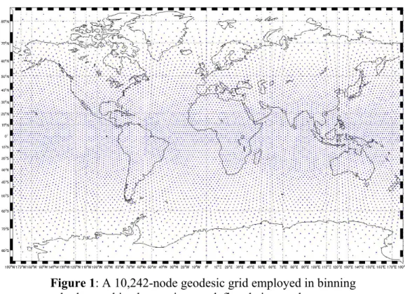
For hydrographic profiles, because their sampling is not spatially regular (i.e., not repeat sampling), sample means are defined according to a geodesic grid with approximately 240km spacing (10,242 nodes; Figure 1). Every profile is identified with its closest geodesic grid point on which the corresponding sample means are computed.
Figure 1: A 10,242-node geodesic grid employed in binning hydrographic observations to define their sample means.
In R3, the TS climatology is used to constrain the estimate’s 24-year mean instead of applying it at monthly intervals as was conducted in R1. Replacing the repeated application of the same data at different instances to a single occurrence, reduces the correlation among the constraints used. Data errors for the hydrographic profiles were also revised from those employed in R1. Errors associated with meso-scale variability not resolvable by the Version 4 model were estimated using the 3-day average output from a nominal 1.2 km horizontal resolution unconstrained forward MITgcm simulation on the llc4320 grid (courtesy Dimitris Menemenlis). The spatial
patterns and magnitudes of these llc4320 variations were found to agree favorably with data errors used in R1 (derived by G. Forget using in situ profile data, following Forget and Wunsch, 2007) with the exception of Arctic and Southern Oceans, where in situ profile data are relatively sparse. In the Arctic and Southern Oceans, errors used in R1 were replaced with the llc4320 variance in R3. In mid and low latitudes, the R3 hydrographic error field is set to be the maximum of the llc4320-derived and in situ-derived fields.
4.2 Reducing spatial correlation
To limit the computational requirements, profile measurements, such as Argo floats, were discretized to 79 distinct levels in R1. However, the vertical resolution afforded by such discretization is higher than that of the model resolution, resulting in correlated model-data differences. To minimize such correlation, profile measurements in R3 were decimated among these levels to no more than the model’s vertical grid resolution.
4.3 Accounting for variations in model grid spacing
Individual constraints in the optimization have been scaled in R3 by their corresponding model area to account for the model’s spatially inhomogeneous resolution. Specifically, prior
uncertainties are normalized (divided) by the square root of the corresponding area of the model grid relative to its largest element (relative area). Such scaling assures that the objective function and its gradients, and thus the optimization, are not dependent on the particular choice of the model grid system.
4.4 Cost function re-formulation
Some of the constraints in the optimization have been re-formulated in R3 to better constrain the model solution. These include constraints for global mean sea level, global mean ocean bottom pressure, and sea-ice concentration. As in R1, sea level observations in R3 are employed “along-track” in the optimization whereby model sea level is constrained when and where the
observations are obtained, leaving unconstrained gaps in the model domain. Estimates of global mean sea level change require data processing to “fill-in” such gaps and to take the observing systems’ instrumental and geophysical corrections into account, including their covariance. To better constrain the model, a separate constraint is employed whereby estimates of global mean sea level change that employ such expert “fill-ins” (scalar time-series) are used to directly
control the model’s mean sea level. Likewise, the model is separately constrained by estimates of global mean ocean bottom pressure change in addition to regional variations of bottom pressure so as to better estimate changes in the model’s integrated mass. In implementing these
constraints, appropriate account is taken of spurious global mean mass and sea level values arising from the Boussinesq formulation of the model.
The model’s sea-ice concentration was constrained in R3 by treating regions with a sea-ice deficit separately from those with excess sea-ice concentration. Where sea ice is observed but not simulated, a penalty is applied to the heat content of the corresponding ocean grid cell equal to the energy required to reduce the grid cell to the freezing point and grow 0.3 m of ice. Where
ocean grid cell equal to the energy required to completely melt the ice and raise the temperature of the grid cell to 1x10⁻⁴ C.
5. Results
The R3 solution is available for download at ftp://ecco.jpl.nasa.gov/Version4/Release3/ (Or go to http://www.ecco-group.org/products.htm and click ECCO-V4 Release 3.) Various climatologies (by year and 20-year averages) are also available as ordinary Matlab .mat files at http://mit.ecco-group.org/opendap/diana/h8_i48/contents.html (The ECCO Consortium, 2017a,b). Different aspects of the R3 solution are illustrated in figures (“standard plots”) assembled in
ftp://ecco.jpl.nasa.gov/Version4/Release3/doc/standardplots.pdf, which can be compared to equivalent plots for R2
(ftp://mit.ecco-group.org/ecco_for_las/version_4/release2/doc/ECCOV4R2_depiction.pdf) and R1
(ftp://mit.ecco-group.org/ecco_for_las/version_4/release1/ancillary_data/standardAnalysis.pdf). Note, however, that in these “standard plots”, a direct comparison of normalized quantities (“cost” in the optimization) cannot be made among the solutions, because many of the uncertainties used to weight the model-data differences are different between the Releases.
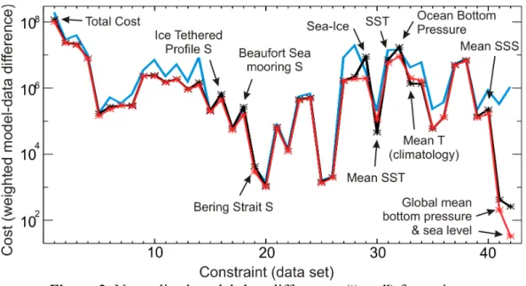
Figure 2: Normalized model-data differences (“cost”) for various observations for Release 2 (black) and Release 3 (red). Also shown are
values for the control run (no optimization; cyan). The quantities are based on the constraints employed in the Release 3 optimization except
the period here is for 1992-2011 (Release 2 period). See Table 4 for description of the different constraints (x-axis).
Figure 2, in contrast, compares weighted model-data differences of R2 & R3 using the same normalization and constraints employed in the latter. (See Table 4 in the Appendix for actual values and a list of the constraints shown in Figure 2.) For most constraints, the model-data differences for the two solutions are comparable to each other and are significantly smaller than those for the control run (i.e., a model simulation without the data constraints, except for using initial temperature and salinity estimated by R2). Larger improvements in cost in R3 over R2 are
found for new observations employed in R3, such as with hydrographic profiles in the Arctic region, ocean bottom pressure, and sea surface salinity, and with new constraints such as sea-ice and global mean sea level. Separating time-mean and time-dependent constraints generally result in a larger time-mean cost (e.g., time-mean SST) but smaller anomaly cost (e.g., SST) in R3 than in R2.
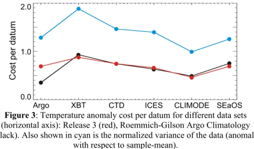
Figure 3 compares R3 temperature anomaly costs (cost per datum) with equivalent measures based on the Roemmich-Gilson Argo Climatology, a monthly mean gridded product of Argo data (Roemmich and Gilson, 2009). Both costs are significantly smaller than the corresponding weighted mean-square value of the observations that is also shown, demonstrating the skill of the two products in resolving the observed variations. While the gridded climatology is closer to Argo measurements themselves, R3 has a more uniform value of model-data differences across the different datasets. Significantly, the R3 values are slightly smaller than those of the gridded product, except for the ICES (International Council for the Exploration of the Sea) measurements in the northeast North Atlantic Ocean. The comparison indicates that as a general description of the ocean, as opposed to a description of Argo data per se, the two products are comparable in skill.
Figure 3: Temperature anomaly cost per datum for different data sets (horizontal axis): Release 3 (red), Roemmich-Gilson Argo Climatology (black). Also shown in cyan is the normalized variance of the data (anomaly
with respect to sample-mean).
What R3 as well as other ECCO products provide, that the gridded Argo product and other observational data sets do not, is the complete suite of variables that describes the entire physical state of the ocean (viz., temperature and salinity throughout the entire water column, as well as sea level, bottom pressure, and velocity). The ECCO products’ variables, unlike in most ocean reanalyses, are physically consistent with each other and with the air-sea fluxes, allowing for a full physical accounting of their temporal evolution fundamental to studies of attribution and causation. An example of such utility is closure of property budgets. Details of how to evaluate budgets using the R3 solution are described in Piecuch (2017). Instructions for reproducing R3 results. for instance, deriving estimates not available in the archive, are described in Wang (2017).
Acknowledgement
This research was carried out in part at the Jet Propulsion Laboratory, California Institute of Technology, under a contract with the National Aeronautics and Space Administration.
References
Chaudhuri, A. H., R. M. Ponte, G. Forget, and P. Heimbach (2013), A Comparison of
Atmospheric Reanalysis Surface Products over the Ocean and Implications for Uncertainties in Air-Sea Boundary Forcing, Journal of Climate, 26(1), 153-170, doi:10.1175/jcli-d-12-00090.1.
The ECCO Consortium (2017a), A twenty-year dynamical ocean climatology: 1994-2013. Part 1: Active scalar fields: temperature, salinity, dynamic topography, mixed layer depth, bottom pressure, (2017-03-20), http://hdl.handle.net/1721.1/107613.
The ECCO Consortium (2017b), A twenty-year dynamical ocean climatology: 1994-2013. Part 2: velocities, property transports, meteorological variables, mixing coefficients, (2017-06-14), http://hdl.handle.net/1721.1/109847.
Forget, G. and C. Wunsch (2007), Estimated global hydrographic variability. J. Phys. Oceanogr., 37, 1997-2008, doi:10.1175/jpo3072.1.
Forget, G., D. Ferreira, and X. Liang (2015a), On the observability of turbulent transport rates by Argo: supporting evidence from an inversion experiment, Ocean Sci., 11(5), 839-853,
doi:10.5194/os-11-839-2015.
Forget, G., J. M. Campin, P. Heimbach, C. N. Hill, R. M. Ponte, and C. Wunsch (2015b), ECCO version 4: an integrated framework for non-linear inverse modeling and global ocean state estimation, Geosci. Model Dev., 8(10), 3071-3104, doi:10.5194/gmd-8-3071-2015.
Forget, G., and R. M. Ponte (2015), The partition of regional sea level variability, Prog Oceanogr, 137, Part A, 173-195, doi:10.1016/j.pocean.2015.06.002.
Forget, G., J.-M. Campin, P. Heimbach, C. N. Hill, R. M. Ponte, and C. Wunsch (2016), ECCO version 4: Second Release, http://hdl.handle.net/1721.1/102062.
Losch, M., D. Menemenlis, J.-M. Campin, P. Heimbach, and C. Hill (2010), On the formulation of sea-ice models. Part 1: Effects of different solver implementations and parameterizations, Ocean Modelling, 33(1-2), 129-144, doi:10.1016/j.ocemod.2009.12.008.
Marshall, J., A. Adcroft, C. Hill, L. Perelman, and C. Heisey (1997), A finite-volume, incompressible Navier Stokes model for studies of the ocean on parallel computers, J Geophys Res-Oceans, 102(C3), 5753-5766, doi:10.1029/96jc02775.
Piecuch, C. G. (2017), A note on evaluating budgets in ECCO Version 4 Release 3. (Available at ftp://ecco.jpl.nasa.gov/Version4/Release3/doc/evaluating_budgets_in_eccov4r3.pdf.)
Piecuch, C.G., P. Heimbach, R.M. Ponte, and G. Forget (2015), The sensitivity of a global ocean state estimate of contemporary sea level changes to geothermal flux. Ocean Modelling, 96(2), 214-220, doi:10.1016/j.ocemod.2015.10.008
Roemmich, D., and J. Gilson (2009), The 2004–2008 mean and annual cycle of temperature, salinity, and steric height in the global ocean from the Argo Program, Prog Oceanogr, 82(2), 81-100, doi:10.1016/j.pocean.2009.03.004.
Wang, O. (2017), Instructions for reproducing ECCO Version 4 Release 3. (Available at ftp://ecco.jpl.nasa.gov/Version4/Release3/doc/ECCOv4r3_reproduction.pdf.)
Watkins, M. M., D. N. Wiese, D.-N. Yuan, C. Boening, and F. W. Landerer (2015), Improved methods for observing Earth's time variable mass distribution with GRACE using spherical cap mascons, Journal of Geophysical Research: Solid Earth, 120(4), 2648-2671,
doi:10.1002/2014JB011547.
Weaver, A., and P. Courtier (2001), Correlation modelling on the sphere using a generalized diffusion equation, Quarterly Journal of the Royal Meteorological Society, 127(575), 1815-1846, doi:10.1256/smsqj.57517.
Wunsch, C., P. Heimbach, R. M. Ponte, and I. Fukumori (2009), The global general circulation of the ocean estimated by the ECCO-Consortium, Oceanography, 22(2), 88-103,
doi:10.5670/oceanog.2009.41.
Wunsch, C. and P. Heimbach (2013), Dynamically and kinematically consistent global ocean circulation and ice state estimates. In: G. Siedler, J. Church, J. Gould and S. Griffies, eds.: Ocean Circulation and Climate: A 21st Century Perspective. Chapter 21, pp. 553–579, Elsevier, doi:10.1016/B978-0-12-391851-2.00021-0.
Appendix: Weighted model-data differences
# Cost Control R2 R3
1 Total Cost 1.21E+08 1.20E+08 9.98E+07
2 Temperature (Argo) 2.38E+07 2.37E+07 2.30E+07
3 Salinity (Argo) 2.11E+07 2.11E+07 2.01E+07
4 Temperature (XBT) 7.93E+06 7.90E+06 7.79E+06
5 Temperature (CTD in Arctic) 1.73E+05 1.70E+05 1.45E+05
6 Salinity (CTD in Arctic) 2.65E+05 2.70E+05 2.28E+05
7 Temperature (CTD in other high latitudes) 2.98E+05 2.96E+05 2.97E+05
8 Salinity (CTD in other high latitudes) 3.02E+05 2.98E+05 2.78E+05
9 Temperature (CTD in low latitudes) 2.35E+06 2.35E+06 2.32E+06
10 Salinity (CTD in low latitudes) 2.34E+06 2.44E+06 2.27E+06
11 Temperature (ICES in high latitudes) 1.45E+06 1.52E+06 1.46E+06
12 Salinity (ICES in high latitudes) 1.87E+06 1.87E+06 1.82E+06
13 Temperature (ICES in low latitudes) 9.18E+05 9.23E+05 8.97E+05
14 Salinity (ICES in low latitudes) 1.31E+06 1.49E+06 1.22E+06
15 Temperature (Ice Tethered Profiler) 2.11E+05 2.08E+05 1.93E+05
16 Salinity (Ice Tethered Profiler) 6.67E+05 6.58E+05 4.41E+05
17 Temperature (Beaufort Sea mooring) 6.39E+04 6.04E+04 5.32E+04
18 Salinity (Beaufort Sea mooring) 2.78E+05 2.70E+05 1.57E+05
19 Salinity (Bering Strait mooring) 4.41E+03 4.31E+03 2.92E+03
20 Salinity (Fram Strait mooring) 1.05E+03 1.09E+03 1.01E+03
21 Temperature (CLIMODE) 6.65E+04 6.69E+04 6.46E+04
22 Salinity (CLIMODE) 1.24E+04 1.24E+04 1.22E+04
23 Temperature (SEaOS) 4.51E+05 4.58E+05 4.22E+05
24 Salinity (SEaOS) 5.10E+05 5.14E+05 4.92E+05
25 Temperature (Davis Strait mooring) 1.42E+03 1.46E+03 1.32E+03
26 Salinity (Davis Strait moorings) 1.85E+03 2.01E+03 1.95E+03
27 Sample-mean Temperature (all in situ profiles) 1.61E+06 1.68E+06 1.63E+06
28 Sample-mean Salinity (all in situ profiles) 2.18E+06 2.23E+06 1.90E+06
29 Sea-ice concentration (satellites) 9.40E+06 8.96E+06 1.97E+06
30 Time-mean SST (satellites) 4.48E+04 4.53E+04 1.09E+05
31 SST (satellites) 7.37E+06 7.31E+06 5.73E+06
32 OBP (GRACE) 1.89E+07 1.74E+07 9.09E+06
33 Time-mean Temperature (Climatology) 1.29E+06 1.36E+06 2.01E+06
34 Time-mean Salinity (Climatology) 1.23E+06 1.35E+06 1.65E+06
35 Mean dynamic topography 5.65E+04 5.88E+04 6.07E+04
36 Sea level (satellite altimetry) 1.35E+05 1.31E+05 1.30E+05
37 Seasonal Temperature (Climatology) 5.09E+06 5.08E+06 4.86E+06
38 Seasonal Salinity (Climatology) 6.93E+06 6.98E+06 6.73E+06
39 SSS (Aquarius) 1.38E+05 1.39E+05 1.26E+05
40 Sample-mean SSS (Aquarius) 2.41E+05 2.25E+05 1.70E+05
41 Global mean OBP (GRACE) 7.87E+02 4.21E+02 2.06E+02
42 Global mean sea level (altimetry) 8.77E+02 2.60E+02 3.29E+01
Table 4: Weighed model-data differences (cost) illustrated in Figure 2. All cost terms are for anomalies unless noted otherwise. SST (sea surface temperature), SSS (sea surface salinity), OBP (ocean bottom pressure)