Dynamic Structural Shape Estimation Using
Integral Sensor Arrays
by
Peter Stewart Lively
Submitted to the Department of Aeronautics and Astronautics
in partial fulfillment of the requirements for the degree of
Master of Science in Aeronautics and Astronautics
at the
MASSACHUSETTS INSTITUTE OF TECHNOLOGY
Feb 2000
©
Massachusetts Institute of Technology 2000. All rights reserved.
A uthor ...
...
Department of Aeronautics and Astronautics
January 28, 1999
Certified
by...
Nesbitt W. Hagood
Professor
Thesis Supervisor
Certified by ..
...
Mauro J. Atalla
Research Associate
Thesis Supervisor
A ccepted by ...
...
Nesbitt W. Hagood
Chairman, Department Committee on Graduate Students
MASSACHUSETTS INSTITUTE OF TECHNOLOGY
Dynamic Structural Shape Estimation Using Integral Sensor
Arrays
by
Peter Stewart Lively
Submitted to the Department of Aeronautics and Astronautics on January 28, 1999, in partial fulfillment of the
requirements for the degree of
Master of Science in Aeronautics and Astronautics
Abstract
Modern structures are becoming intelligent structures, with embedded sensors and actuators. This is particularly true for aircraft where any extra weight is costly. Shape estimation is one technique that can utilize embedded sensors to improve the aircrafts performance. Having shape knowledge allows for embedding phased antennae arrays into large structural surfaces such as wings. The shape information is used to adjust the phasing for optimal signaling. Another application is for HALE aircraft, where the flexible wings are vulnerable to gusts. Shape estimation allows a controller to steer through the gust to avoid failure.
Currently the most robust method of shape estimation utilizes global shapes, which are generally the lowest structural modes. These modes produce the greatest levels of deflection. The sensor readings, usually strain gages, are passed through a weighting matrix which provides an estimate of the modal amplitudes. Summing the amplitudes provides and estimate of the total shape. This has been shown to provide accurate results for static structures. Current dynamic shape estimation techniques use the static technique for each time step. The aliasing of the higher modes, which is largely not seen in the static case, occurs strongly in the dynamic case. Higher frequency modes cause high strain with relatively little displacement. In many cases the aliasing produces signal to noise ratios significantly greater than unity.
This paper presents a new technique that uses the dynamic model of the structure to greatly reduce the effects of aliasing. The premise is to use a Kalman filter to sift out the desired low frequency modes and treat the higher modes as part of the noise. Also, unlike the static techniques, the Kalman filter allows sensing of more modes than there are sensors and takes into account the strain gauge errors. Numerical analysis shows that the Kalman filtering technique can reduce the error from a thousand percent down to less than a percent in an ideal case. Including sensor noise and modeling error reduces the efficacy of the method but still produces a significant improvement.
Thesis Supervisor: Nesbitt W. Hagood Title: Professor
Thesis Supervisor: Mauro J. Atalla Title: Research Associate
Acknowledgments
A number of people helped me get my experiment off the ground, and they most of
all should be thanked. So thanks Mauro, Michael, Cagri.
But most of all I would like to thank the people that helped me the last few weeks, even if they didn't know it. Thanks Michael, John, Mary, Will, John and my little
Contents
1 Introduction
1.1 Intelligent Structures . . . . 1.2 Modal Detection and Sensing . . . . .
1.3 Shape Estimation . . . . 1.4 Design Requirements . . . . 2 Methodologies 2.1 Introduction . . . . 2.2 A liasing . . . . 2.3 Static Methods . . . . 2.3.1 Introduction . . . . 2.3.2 Sensors. . . . . 2.3.3 Shaped Sensors . . . . 2.3.4 Integration Methods . . . .
2.3.5 Global Shape Estimation . . . .
2.4 Dynamic Methods . . . . 2.4.1 Selection of Base Method . . . .
2.4.2 Quasi-Static Shape Estimation.
2.4.3 Temporal Filtering for Quasi-Static Shape Estimation 2.4.4 Kalman Filtering . . . . 2.5 Summary . . . . 14 14 15 16 18 20 20 21 22 22 22 22 24 25 26 26 27 28 29 31
3 Numerical Simulations 32
3.1 Introduction . . . . 32
3.2 Beam Simulation . . . . 32
3.3 Quasi-Static Shape Estimation . . . . 35
3.3.1 Ideal Model with no Sensor Noise . . . . 36
3.3.2 Ideal Model with Sensor Noise . . . . 40
3.3.3 Effects of Modeling Errors . . . . 41
3.4 Quasi-Static Shape Estimate with Temporal Filter . . . . 44
3.4.1 Ideal Model with no Sensor Errors . . . . 44
3.4.2 Ideal Model with Sensor Errors . . . . 44
3.4.3 Effects of Modeling Errors . . . . 47
3.5 Kalman Filter . . . . 47
3.5.1 Ideal Model with no Sensor Noise . . . . 50
3.5.2 Ideal Model with Sensor Noise . . . . 51
3.5.3 Effects of Model Error . . . . 53
3.6 Method Comparison . . . . 56 3.7 Sum m ary . . . . 61 4 Experiment 62 4.1 Experimental Setup. . . . . 62 4.2 Model Determination . . . . 65 4.3 R esults . . . .. . . . . 67 4.3.1 M odel . . . . 67 4.3.2 Experimental Results. . . . . 76 4.4 A nalysis . . . . 79 4.5 Sum m ary . . . . 96 5 Conclusions 97 5.1 Sum m ary . . . . 97
A Additional Simulation Results 100
B Conversion of Continuous State Space Model to Discrete Form 104
C Matlab Simulation Code 107
C.1 Finite Element Model ... 107
C.2 Simulation Code ... ... 112
C.3 Experiment Analysis Code ... 119
C.4 Kalman Filter Code for Experimental Analysis . . . . 123
D Matlab Experiment Code 127 D.1 Experiment Code . . . . 127
List of Figures
2-1 Typical Example of a Discrete Shaped Sensor . . . . 24
3-1 Sensor Locations for 1, 2, 4, 6, 8 and 10 Sensor Cases . . . . 34
3-2 Bode Magnitude Plot of Actual Deflection vs. Estimated Deflection
For Quasi-Static Shape Method with 1 Sensor . . . . 37 3-3 Average Fourier Transform of Actual Deflection vs. Estimate Error for
Quasi-Static Shape Method with 4 Sensors . . . . 38
3-4 Time History of Actual Deflection and Quasi-Static Estimate . . . . . 39 3-5 Estimation Error as a function of Sensor Noise and Number of Sensor
for Quasi-Static Shape Method . . . . 40
3-6 Fourier Transform of Quasi-Static Estimate with 20% sensor noise and
4 sensors . . . . 42
3-7 Results of Modeling Error on Quasi-Static Shape Estimation Error . . 43
3-8 Tip Deflection Estimate Errors for the Filtered Quasi-Static Method . 45
3-9 Sensor Noise effects on Quasi-Static Estimate with Filtering . . . . . 46
3-10 Effects of Modeling Error on Quasi-Static Estimate with Filtering . . 47
3-11 Time History of Actual Displacement and Kalman Estimates . . . . . 49
3-12 Kalman Filter Error for System without Sensor Noise . . . . 50 3-13 Comparison of Fourier Transforms for 4 and 8 mode Kalman Filter 52
3-14 Kalman Filter Errors without Noise and with 20% Noise . . . . 54
3-15 Effect of Modeling Error on Kalman Filter Estimation Error . . . . . 55
3-16 Effect of 20% Sensor Noise on Kalman Filter with Modeling Error . . 57
3-18 Comparison of Methods for Ideal System without Sensor Noise . . . . 59
3-19 Model Behavior as a Function of Sensor Noise for Beam with 10 Sensors 60
4-1 Photograph of the Experimental Setup Showing the Strain Gage Lo-cations . . . . 63
4-2 Photograph of the Experimental Setup Showing the Laser Vibrometer and PZT Actuator . . . . 64 4-3 Measured Drawing of Experimental Setup . . . . 65
4-4 Transfer Function showing Amplifier Dynamics . . . . 66
4-5 Experimental vs. Modeled Transfer Functions for Tip Deflection . . . 69
4-6 Experimental vs. Modeled Transfer Functions for Root Strain Gage . 70
4-7 Experimental vs. Modeled Transfer Functions for Second Strain Gage 71
4-8 Experimental vs. Modeled Transfer Functions for Third Strain Gage . 72
4-9 Experimental vs. Modeled Transfer Functions for Fourth Strain Gage 73
4-10 Experimental vs. Modeled Transfer Functions for Fifth Strain Gage . 74 4-11 Sensor Locations on Predicted Strain Modes . . . . 77
4-12 Estimated Modal Amplitudes using Quasi-Static Method . . . . 78
4-13 Time History of Quasi-Static Estimate vs. Actual Displacement . . . 80
4-14 Time History of Filtered Quasi-Static Estimate vs. Actual Displacement 81 4-15 Time History of Modally Filtered Quasi-Static Estimate vs. Actual
D isplacem ent . . . . 82
4-16 Time History of the 8 Mode Kalman Filter Estimate vs. Actual Dis-placem ent . . . . 83
4-17 Power Spectral Density of the Quasi-Static Estimate vs. Actual Dis-placem ent . . . .. . . . 85
4-18 Power Spectral Density of the Filtered Quasi-Static Estimate vs. Ac-tual Displacem ent . . . . 86
4-19 Power Spectral Density of the Modally Filtered Quasi-Static Estimate vs. Actual Displacement . . . . 87
4-20 Power Spectral Density of the 5 Mode Kalman Filter Estimate vs.
Actual Displacement . . . . 89
4-21 Power Spectral Density of the 8 Mode Kalman Filter Estimate vs. Actual Displacement . . . . 90
4-22 Power Spectral Density of Estimates for the First Mode . . . . 91
4-23 Power Spectral Density of Estimates for the Second Mode . . . . 92
4-24 Power Spectral Density of Estimates for the Third Mode . . . . 93
4-25 Power Spectral Density of Estimates for the Fourth Mode . . . . 94
List of Tables
3.1 Quasi-Static Estimation Error due to Sensor Noise
3.2 Quasi-Static Method, Effects of Model Error . . . 3.3 3.4 3.5 3.6 3.7 3.8 3.9 4.1 4.2 4.3
Filtered Quasi-Static Estimation Error, Effects Filtered Quasi-Static Estimate Error, effects of Terse Kalman Filter, Effects of Sensor Noise Full Kalman Filter, Effects of Sensor Noise Terse Kalman Filter, Effects of Model Error Full Kalman Filter, Effects of Model Error Estimation Error for Methods . . . .
Modal Frequencies and Damping Ratios . . .
Experimental Gains . . . . Experimental Results . . . .
of Sensor Noise Modeling Error
A.1 Quasi-Static Method - Accurate Model, No Error . . . .
A.2 Quasi-Static Method - With 5% Model Error . . . .
A.3 Quasi-Static Method - With 20% Model Error . . . . .
A.4 Quasi-Static Method With Filtering -Accurate Model, No Error
A.5 Quasi-Static Method With Filtering - With 5% Model Error
A.6 Quasi-Static Method With Filtering - With 20% Model Error
A.7 Exact Kalman Filter - Accurate Model, No Error . . . .
A.8 Exact Kalman Filter - With 5% Model Error . . . .
A.9 Exact Kalman Filter - With 20% Model Error . . . .
A.10 Extended Kalman Filter - Accurate Model, No Error . . . .
. . . . . 41 . . 43 . . 46 . . 48 51 53 56 56 59 75 75 79 100 101 101 101 101 102 102 102 102 103
A.11 Extended Kalman Filter - With 5% Model Error . . . . 103 A.12 Extended Kalman Filter - With 20% Model Error . . . . 103
Chapter 1
Introduction
1.1
Intelligent Structures
Intelligent structures are being used increasingly for hi-tech projects particularly for aerospace vehicles and applications [25, 28]. An intelligent structure utilizes integral sensors and actuators to increase performance. These integral systems can either augment or replace their on-board counterpart.
Warkentin et al. [33, 34, 35] worked extensively on embedding electronic compo-nents into a composite structure and modeling the resulting structure. Of particular importance is embedding piezoelectric actuators and correctly predicting their behav-ior. Their work on modeling of the piezoelectric materials allows for the piezoelectric materials to be used efficiently, and to develop algorithms for optimal placement for control applications.
John Rodgers, et al. [29] have used embedded Active Fiber Composites (AFC) in the construction of an active twist rotor blade. The active rotor blade has the advantage of high bandwidth actuation allowing for control of higher modes. These blades will be able to reduce the noise produced by helicopters, increasing performance and comfort levels. Another benefit is that it allows for simplification of the hub machinery, increasing life of the helicopter as a whole.
Embedded arrays of PZT's were used by Mark Lim and Fu Kuo Chang [30, 24] to create a method of damage detection. The PZT's act as both actuators and
sensors, where one of the PZT's is used to send out a high frequency strain burst that is picked up by the other embedded PZT's. The undamaged baseline is compared to subsequent readings. Increases in time lag and scatter indicate damage in the structure. Comparing the various lag readings and levels of scatter the damage can be located within the structure.
1.2
Modal Detection and Sensing
For many control applications modal detection is important. Lee and Moon [23] have developed a method for shaping sensors to sense one particular mode. The spatial shape of the sensor is determined to provide a signal proportional to the desired mode. This shape is also created to be orthogonal to the undesired modes. Burke and Hubbard [7] also developed similar ideas that are used for modal control of a beam. Unfortunately this requires very large sensors that take up most of the structural area.
For many structures Viri and Heyns [32] have shown that the strain shapes are not necessarily orthogonal. The total deformation energies of the structure maintain their orthogonality, but that includes deformations at the boundaries which cannot be included in any simple manner.
Miller et. al. [26] developed shaped sensors that are local rather than distributed. The spatial shape of the sensor detects spatial waves of a certain length. The length of the spatial wave corresponds to a structural frequency, with longer waves correspond-ing to lower frequencies. The size and shape of the sensor determines the roll-off point and rate respectively. These shaped sensors are very useful to reduce the sensitivity to high-frequency modes. These are particularly useful for long slender applications, such as beams and rods where the spatial sensitivity of the sensor can be controlled
by adjusting the transverse width. The transverse sensitivity of the sensors makes
this much more difficult on a plate structure.
Han and Lee [16] used an array of piezoelectric sensors and actuators to control the deflections of a cantilevered plate. The plate was covered with piezoelectric patches
and the system was identified. Boolean weightings were applied to each of the sensor patches to best isolate the first mode of the structure, and reduce the observability of the higher modes. A similar weighting system was applied to the actuator piezos. The resulting configuration showed very good performance at reducing the controlled mode without detriment to the higher modes. This approach has a number of shortcomings however. The sensors layout once chosen was hardwired in, and any changes to the structure would dramatically alter performance.
Michael Fripp [13] has investigated the use of an array piezoelectric sensors with continuous weightings for vibration and structural-acoustic control. The weightings are chosen to correspond to the modes of interest, which are to be controlled. The sen-sor weightings are determined from the sensen-sor transfer functions and can be updated with changes in the structural response.
1.3
Shape Estimation
The need for Shape Estimation in an intelligent structure is becoming more apparent.
GPS booms, for example, require very precise alignment where a 0.1 degree error in
alignment can cause a 0.5 mile ground error [21]. Another precision shape application is for conformal antenna arrays for high performance aircraft. The antenna is built into the wing of the aircraft and requires very precise alignment[20].
Shape estimation draws upon various aspects of intelligent structures, primarily the use of arrays of sensors. The larger the array of sensors the better the estimate becomes. Additionally, shape estimation can utilize sensors already in place for other purposes, such as strain monitoring, or acoustic damping.
The basis for most higher-order shape estimation techniques is to map displace-ment fields to strain fields. Foss and Haugse [12] used large arrays of strain gages and accelerometers to map strain shapes and the corresponding deflection shapes. The testbed was a cantilevered plate. They isolated individual modes and used curve fitting techniques to interpolate between sensor locations. The final result is accurate strain shape maps and displacement mode shapes.
Mark Andersson [2] investigated the use of arrays of shaped sensors for shape estimation. His work included comparisons of integration techniques to modal sensing techniques, as well as the effects of shaped sensors and the number of sensors on these results. The results varied depending on the scheme used and the sensor, but the trend was that a larger number of sensors produced more favorable results, and that shaping the sensors had marginal effects in most cases.
Not all shape estimation methods use a strictly strain gage approach though. Baz and Poh [4] developed a wire gage that does point estimations of the slope of the beam through integration of the strain down the length of the wire. Their work included using an oscillating platform to actuate a beam that is clamped to it. This allows them to excite the beam at specific frequencies. Their results were rather accurate, but they only conducted tests at low frequencies.
The major shortcoming with the shape estimation performed to date is that little has been done for a vibrating structure. Kirby et. al. [21] performed experiments on a structure undergoing a step loading, using strain integration techniques. The transient results proved accurate, but there was a high level of error immediately after the step load that is unaccounted for analytically. Much of this error is undoubtedly from the aliasing effects of the high frequency modes that are not accounted for with standard static shape estimation techniques.
The purpose of this work is to develop a strategy to address the aspect of dynamics in shape estimation. To do this modal estimation techniques developed for controls applications are applied to current shape estimation techniques. Sensor weighting functions are the most basic techniques, and are already being utilized in the global shape estimation method. More advanced methods filter the signal in frequency, as the weighted sensors are designed to filter the response spatially.
Modal estimation techniques thus provide a better estimate of the modal am-plitudes, that are then combined with the mode shapes to render a final deflection shape.
1.4
Design Requirements
In designing a dynamic shape estimation method it is important to recognize and design toward certain performance and functional requirements. A methodology that works poorly is worse than not having one at all.
The primary performance requirement for a shape estimation method is that the error in the estimated shape must be less than the actual deflection levels. Any method that produces greater error than the deflection level is worse than assuming no deflection at all.
In order to reduce the errors in the system, the method must be able to account for four different types of errors:
1. Aliasing of higher modes
2. Truncation of the model
3. Sensor error
4. Model error
The importance of these errors is dependent on the number of sensors, sensed modes, bandwidth of the external forcing and model accuracy.
Aliasing errors occur for two reasons in a dynamic system. The primary reason is that the sensor weighting matrix is only capable of differentiating between as many modes as there are sensors. Higher modes are thus interpreted as combinations of the lower modes, often producing very large errors. The second form the aliasing takes is digital aliasing due to the rate of sensing. If the bandwidth of the sensing is suitably high, this does not have much effect however.
Model truncation is, in a way, the opposite of aliasing. Model truncation occurs because not all of the structural modes can be added to the total deflection. The estimated deflection reflects the truncation by not having those modes appear in the estimate. This means that the estimated deflection will necessarily be simpler than the real deflection. The effects of model truncation are not as severe for shape estimation as they are for controls, since deflection rolls-off very quickly with frequency.
an intrinsic level of error, due to sensitivity limitations, line noise, drift, etc. Beyond that, there is also error due to misalignment and incorrect placement of the sensor. Small errors in the location of the sensor can have profound impact on their reading especially for higher modes that have short spatial wavelengths.
Model error is the last of the main causes of errors in the system. No matter how sophisticated the finite element package, or the identification software, the structure is not going to be modeled entirely correctly. This is especially true for a structure that is subjected to changes in environment, i.e. hot to cold, or operates in a rugged environment where it will be damaged, since damage changes the structural response. For this problem the two main sources of model error are errors in modal frequencies and physical mode shape.
In addition to having to contend with the various sources of error, the technique must also be fast, a restriction that does not exist for static shape estimation. The dynamic technique should be capable of updating the estimated shape as quickly as new information is available. At the minimum the system rate should be less than the Nyquist frequency for the highest desired mode (wma,/2).
Additional requirements on the performance and functioning can be made as nec-essary for the specific applications. In general the above and an absolute tolerance on the deflection error at any point suffice to delineate the problem.
The next chapter will go into more detail on the various methodologies that are available for shape estimation, including discussion on the relative merits of each method. Following the methodologies chapter is a chapter on the computer simula-tions that were run using the various temporal filters. The experimental results are presented after the computer simulations.
Chapter 2
Methodologies
2.1
Introduction
Static shape estimation is the basis for the dynamic methods used in this work. The most basic shape estimation method is simply iterating the static method, while the more complex methods fit dynamic modes to the sensor readings.
In tailoring a static shape estimation method to a specific structural application, a number of parameters must be determined. One must first determine the number, the type, and the locations of the sensors. It is also important to consider whether the number and location of sensors is a fixed parameter or a design parameter.
No matter what method is used, shape estimation starts with some type of model of the structure. This creates a way to relate the readings of the sensors to what is physically happening in the structure. For the simpler methods all that is required is the geometry of the structure. As the methods get more complicated the necessary complexity of the model also increases.
When selecting a methodology for shape estimation the first step is to examine the potential errors, modeling errors, sensing errors, aliasing, etc. Of the possible errors, the presense and potential degree of aliasing is the easiest to predict and design for. Based on the types and estimated levels of errors, an underlying static method can be chosen. The static method determines how the sensor information is used spatially. After choosing a static method, a dynamic method can be added. The
dynamic method uses temporal information to improve the spatial information in the static method.
2.2
Aliasing
As the leading cause of errors in a shape estimation method it is important to under-stand exactly what causes the aliasing and how great its effect really is. The manner and degree that aliasing affects the sensors will help determine which method should be used.
Aliasing occurs when one mode is mistaken for another mode, or combination of other modes. In the case of shape estimation this means that the strain produced
by an unsensed mode is aliased to the strain from the sensed modes. This produces
erroneous readings for the sensed modes causing errors in the estimated shape. In a structure with few sensors and high bandwidth noise, aliasing can be disas-trous, easily causing errors that completely mask the underlying signal. Each addi-tional sensor decreases the error significantly. A lower bandwidth for the noise means that the higher modes do not get excited as much, and are less able to cause aliasing. Mathematically the cause of aliasing can be demonstrated by examining a vibrat-ing beam. Equation 2.1 shows the governvibrat-ing differential equation for a vibratvibrat-ing beam. For an infinite beam, the transfer function corresponds to the dereverberated transfer function of a generic beam, as shown in Equation 2.2, where the structural wavelength A c< 1/vlw.
pz + EIzIV = F(x, t) (2.1)
z(x, t) = sin(wf + )7 (2.2)
This results in a curvature that is proportional to 1/w. This means the curvature to displacement transfer function is proportional to:
X(W)= W (2.3)
Since the strain gage reading is directly proportional to the curvature, this means that the sensor to displacement function rolls up with frequency, which is very un-desirable from a controls point of view. The results of this is that the higher modes have proportionally greater influence on the sensed deflection than the lower modes.
2.3
Static Methods
2.3.1
Introduction
Static Methods are the shape estimation techniques that are used for a structure undergoing static deformation, or very low frequency deformation. Static methods are also the first step in creating a dynamic shape estimation method.
2.3.2
Sensors
A strain gage attached to the surface of a bending structure will respond linearly
with local curvature. Ideally a pair of strain gages are utilized on opposing sides of the structure. The use of two strain gages allows for compensation for elongation of the structure. Mid-plane deformation produces strain on both sides of the structure with the same sign, whereas curvatures produces strains of opposing signs.
Typically in a thin structure the strains due to curvature will be much greater than those due to mid-plane deformation. This is especially true for beam-like structures which have large transverse loads and small, if any, loads down the length of the structure. This means that a single strain gage on one side of the structure will usually suffice.
2.3.3
Shaped Sensors
A strain gage is not a point sensor. The output signal is in reality the integration
of the strain over its entire area. Typically this is not a factor in the use of a strain gage, although it may help determine a size requirement.
Using piezo-electric material it is possible to specifically shape the strain gage's area to improve sensing. This is usually done in one of two ways, global strain gages and discrete strain gages.
Global Strain Gages
Global strain gages are used to pick out a single mode in a deformed structure. The gage is shaped in such a way that the output of the sensor is proportional to the deformation for that mode. The gage is also shaped so as to be orthogonal to the other modes of the structure.
Designing a Global Strain Gage starts with either a very detailed computer model of the structure, or with a detailed physical identification of the structure to be sensored. The next step is to look for regions that have high strain for the desired modes, and low strains for the other modes. To complicate the matter the sensor should be designed to be entirely contiguous. Charette and Berry [8], and Lee and Moon [23] investigated ways to accomplish this. The disadvantage of this method is that the sensor must often be subsequently tailored to account for the sensors weight and stiffness which alter the structural modes. Additionally only a limited number of such sensors are capable of being used on a structure at one time since they cover such large areas.
Discrete Shaped Strain Sensors
A discrete strain gage works on a fundamentally different idea than a globally shaped
strain gage. A discrete strain gage is designed to act as a spatial filter for strain waves. The discrete gages cannot be used by themselves to determine deflection, but must be coupled with another shape estimation method. The purpose of the discrete gage is to help filter out the higher modes of the structure.
Discrete shaped strain gages are typically used in a beam structure where most of the strain is in the same direction. This simplified structure allows the assumption that the strain field is invariant across the width of the beam and varies only along the length of the structure. This means that the width of the gage can be used to
Sensor
Beam
Figure 2-1: Typical Example of a Discrete Shaped Sensor
determine the magnitude of the gage's response at any point along the length of the gage.
Typical discrete gages are shaped in the same way the time signatures for low-pass filters are designed. The idea is for long strain waves to give strong signals and for shorter strain waves to be attenuated. The shorter strain waves correspond to higher frequency modes which are typically undesirable for shape estimation, whereas the longer modes dominate the deflection. A typical example of a spatially filtering strain gage is illustrated in Figure 2-1.
On two dimensional structures the width of the gage is not a feasible design parameter since piezoelectric materials, which is the typical sensor type used for shaped sensors, have high transverse sensitivities. However, even though a beam structure is the easiest for which to design a discrete filter, other structures are capable of utilizing shaped sensors. A circular gage for instance increases the roll-off of the strain gage, compared to a rectangular gage, from 1/w to 1/w2 [2].
2.3.4
Integration Methods
The most straight forward class of the shape estimation methods is integration tech-niques. Since the strain gages mounted on the surface of the structure measure the local curvature, the curvatures can be integrated to determine the deflection.
Almost any integration method can be used for shape estimation. Higher order methods tend to produce better results however. Gaussian integration for instance
effectively doubles the number of strain gages through careful placement of those sensors to be orthogonal to higher modes that do not contribute to deflection. Even without being able to choose the location of the sensors, integrations techniques can be very powerful.
There are however a number of drawbacks. The first is that integration techniques are very difficult to use on complicated structures; their usefulness is basically limited to beams and very simple plate structures. An additional difficulty, specific to using integration methods for dynamic shape estimation, is that the better integration methods are computationally expensive relative to other methods [3].
2.3.5
Global Shape Estimation
Global Shape Estimation is basically the opposite of integration methods. Global Shape Estimation starts with estimated shapes and differentiates them twice to find the curvatures. A matrix correlating the curvatures, which are also the strain gage readings, to the global deformation shapes can thus be created. Inverting this matrix gives the sensing matrix.
Multiplication of the sensing matrix by the sensor readings directly produces the modal amplitudes. Since each mode has a predetermined mode shape corresponding to it, the modal amplitudes can then be multiplied by the displacement curves for their respective mode. Summing the resulting curves gives an estimate of the shape of the structure.
Global Shape Estimation has a number of advantages over the other methods, especially for structures undergoing dynamic deformations. Since the shapes are predetermined, a number of other aspects of the structure can be identified with the same sensors and mode shapes, including information such as stress levels, and slopes which are useful for pointing applications. By examining consecutive time steps, accelerations and velocities can also be determined directly.
Global Shape Estimation also has the advantage of being very easy to adapt to different structures. Once the model of the structure is created and mode shapes are determined, the sensing matrix can be formed, and then the system is ready. For a
dynamic structure the model can even be created by identifying the structure [12]. In terms of suitability for dynamic shape estimation, the global methods are also very good. The time required for the matrix multiplications is very small compared to the calculations required by some of the integration methods.
The primary disadvantage of the sensing global shapes is that there are no innate anti-aliasing features. The complexity of the deformations that can be sensed is proportional to the number of sensors. More specifically the number of mode shapes that can be distinguished is equal to the number of sensors.
2.4
Dynamic Methods
2.4.1
Selection of Base Method
In order to compare accurately the results of different dynamic methods, it was de-cided that a single base static method should be used. Global Shape Estimation was concluded to be the best choice. The global shapes that the methods will utilize are the deflection mode shapes of the structure.
There are many advantages to using Global Shape Estimation. It has been shown that this is a very reliable and accurate method for determining the deflection of a static structure [1, 2, 3, 21]. Also, unlike methods methods such as curve fitting, it is very quick to implement requiring a simple matrix multiplication to get the results.
There are a number of reasons the dynamic mode shapes are used for the shape estimation. First of all, the dynamic mode shapes are the easiest to find. Finite element methods and dynamic models of the system find and use the dynamic modes. The dynamic modes also correspond to the lowest energy modes of the structure, which are also the preferred modes for deformation. Thus the dynamic modes are the modes that are determined by the structure itself.
2.4.2
Quasi-Static Shape Estimation
Quasi-Static Shape Estimation is the simplest way to create a shape estimation method for dynamic systems. The premise is to perform a separate static estimate of the structure's shape at each time step. The dynamics of the structure are not considered only the instantaneous readings of the sensors.
Although the dynamics of the structure are not considered, it is best to use the dynamic modes of the structure as the interpolation shapes. Once these modes are found the sensor readings for each mode is determined and put into a matrix, see equation 2.4. For a structure with n sensors, up to n modes can be sensed. The
C matrix1 is inverted, or pseudo-inverse if fewer than n modes are being sensed, to
produce the sensor matrix S. The sensor matrix is then used to determine the estimate of the modal amplitudes, i, as shown in equation 2.6 . In the absence of noise or aliased modes this will produce exact results.
Z =Cr (2.4)
S =O-1 (2.5)
r,=SZ (2.6)
This method has a number of advantages over more complicated methods. The first advantage is that it is by far the quickest method and the least computationally expensive. If there are only a few positions that need a deflection estimate, such as tip deflection or pointing, then Quasi-Static estimates can even be programmed with analog devices.
Another advantage is that the Quasi-Static method does not require additional calculations to correctly sense a static offset in position. This is most useful for structures that have very low bandwidth loadings or for deformation loadings rather than force loadings. This method is also the least susceptible to changes in the structure, since most changes would change the dynamics of the structure but not
the overall stress distribution.
The main disadvantage of Quasi-Static Shape estimation is that it is the most sensitive to aliasing of unsensed modes. If the bandwidth on the loading is below the frequency of the last sensed mode, then the quasi static method is usually sufficient. However as the noise bandwidth increases the effects of the aliasing increases as well.
2.4.3
Temporal Filtering for Quasi-Static Shape Estimation
The greatest disadvantage of the Quasi-Static method is its susceptibility to aliasing of higher modes, which will be shown in both the computer simulation chapter and the experimental chapter. The obvious solution to the aliasing is to filter those modes out. On a static structure the only method to do this is through shaped sensors, but on a dynamic structure it is possible through the use of a temporal filter. Algebraicly this is easy to show, by combining equation 2.6 with a filter F(t) as shown in equation 2.7.
f = SZ * F(t) (2.7)
Every dynamic deflection mode of a structure has a corresponding frequency, with the higher modes having higher frequencies. Using a low pass filter it is possible to filter out the high bandwidth signals from the sensors and allow the low frequencies to pass through. Setting the cutoff frequency of the filter to be between the sensed and the unsensed modes should reduce the effect the aliased modes have on the deflection shape and allow the sensed modes to go through unaffected. Incidentally the same result can be obtained by using the temporal filter after the shape has been estimated because the shape estimation method is linear.
The advantages of this method are considerable. The only difference between this method and the Quasi-Static method is the addition of a low pass filter. This means that the implementation is quite simple and the only additional information that is needed is the approximate modal frequencies.
The inherent disadvantage of this method is that information is lost. While it is desirable to ignore the higher modes to prevent aliasing, the information could still
be made useful in some other form.
An additional disadvantage is that any filter will add lag to the system. The amount of lag depends on the type of filter that is used. Generally the lag mainly effects the modes closest to the roll-off, so in systems with greater numbers of sensors and sensed modes, the effects will be less than for systems with few sensors.
2.4.4
Kalman Filtering
The final method that will be considered is the use of a Kalman filter to determine the modal amplitudes. The Kalman Filter [5] was designed for systems with noisy sensors where the plant dynamics are known a priori. The principle is to propagate the modal information forward for each time step. The sensor information readings are compared to the propagated states and new states are determined.
Design of a Kalman Filter starts with a state space model of the structure. Unlike the limited model used for Quasi-Static estimation, this model includes estimates of the errors and the forcing of the structure. For the estimation to be true least squares, the errors and forcing should be white noise with zero mean2. The states
of the system are the modal amplitudes and the modal velocities. Unlike the Quasi-Static methods, the Kalman filter can estimate more modes than there are sensors, and it is advantageous to include as many modes as can be accurately modeled.
Xk = 4DXk-1 + v (2.8)
Zk = Hxk + n (2.9)
The Kalman Filter uses the discrete state space model3 as illustrated in
equa-tions 2.8 and 2.9. Eq's 2.10-2.14 show how the Kalman filter is used in practice. The (-) superscript indicates values that are propagated forward in time before new information is added, and the (+) superscript indicates the current values with the
2
There are methods of designing Kalman filters for non-zero mean and colored noise, see Brown [5].
3
Derivation of the variables from continuous state space form to discrete state space form is detailed in Appendix B or in Brown [6].
inclusion of the new information. Xk = <bXk_1 (2.10) P -= <DPk_1DT +
Q
(2.11) Kk = P H T (HP H T + R)- 1 (2.12) k= i Kk(Zk - Hx-) (2.13) Pk = (I - KkH)P (2.14)The H matrix is the sensing matrix, which contains the sensor readings if there is no sensor noise. The P matrix is the covariance of the uncertainties for the states. The most important value is K, which is also called the Kalman gain. The Kalman gain is the weight applied to the sensor readings, as opposed to using the previous estimate propagated forward in time.
There are a number of advantages to using a Kalman Filter. The first is that it has inherent anti-aliasing ability, in that the Kalman Filter is able to differentiate between signals of different frequencies even if they have the same spatial weightings. A Kalman filter does this by estimating more modes than there are sensors. Estimating additional modes also produces less errors due to truncation.
The Kalman Filter is also a good approach because it does not require filters or storage of previous data points. The amount of lag that is produced is also consider-ably less that for other methods of filtering.
Although in general the Kalman Filter is very good, it does have a few disadvan-tages. The first is that it requires a model of the system. If the model is inaccurate the Kalman Filters suffers more than other methods. The Kalman Filter also takes more time to run than the Quasi-Static system. Generally the Kalman Filter is still capable of running in real time, but for very high bandwidth systems alterations have to be made.
Inherent in the Kalman Filter is the assumption that the input noise and the structural forcing obey zero mean white noise restrictions. This is not generally the
case especially in loaded structures. Additional modes must be used to estimate the force bias [5].
2.5
Summary
There are a number of different shape estimation methods available, each with inher-ent advantages and disadvantages. More simple structures favor the more powerful methods, such as integration, where more assumptions about the behavior of the structure can be made safely. A more complicated structure favors simple methods such as global shape estimation.
Using a global shape estimation method, with the interpolation shapes equivalent to the mode shapes, allows the use of dynamic methods. The dynamic methods are designed, primarily, to alleviate the effects of aliasing. Methods including temporal filtering and Kalman Filtering are considered.
Chapter 3
Numerical Simulations
3.1
Introduction
In order to verify the usefulness of applying dynamic methods to shape estimation numerical trials were performed. The trials consisted of using a finite element model of a beam undergoing white noise excitation. The modeled beam includes models of strain sensors distributed along the beam.
The information from the model strain sensors is passed through the various dy-namic methods to obtain estimates of the tip deflection. The results are compared to the average tip deflection.
There are three primary types of trials that were conducted. The first is a perfectly modeled structure with perfect sensors, using Different numbers of sensors. The second set of trials adds sensor noise of various levels. The final type of trial adds
modeling error and sensor noise to try to better represent a real structure.
3.2
Beam Simulation
The canonical problem for shape estimation has always been the cantilevered beam. The beam is a simple enough structure that it is generally easy to model, and for a cantilevered beam the mode shapes and frequencies are well known. An additional advantage of using a cantilevered beam is that the tip deflection is an ideal metric to
check the accuracy of the method.
The beam modeled in the simulations corresponds very closely to the actual beam that was used in the experiments. The modeled beam was steel, measuring .381 meters in length, and 1.016 mm thick, with Young's Modulus 210 GPa, and specific weight of
7.850. The resulting fundamental frequency is 36.7 rad/sec. The forcing used in the
simulations was a transverse tip force. This does not mirror the experiment, described in the next chapter, because the tip loading provides clearer transfer functions for analysis as well as ensuring that all modes are forced.
The simulations performed here use a finite element model of a cantilevered beam with 240 Bernoulli Euler Beam finite elements. The number of elements was set to allow ample resolution and accurate mode shapes. The first 25 modes of the structure are retained for the dynamic simulation of the structure. Fewer modes would have made the modeling inaccurate due to truncation errors, and more modes were determined to be superfluous since the contribution to the deflections and strains were so small.
Each of the cases was run for a system with 1, 2, 4, 6, 8, and 10 sensors that are evenly distributed along the length of the beam with the first sensor always going at the root, i.e. for 4 sensors they go at the root, at 1/4 L, 1/2 L and 3/4 L. These locations are shown in Figure 3-1 overlaid on the second displacement mode. The sensors are modeled as being 4 elements in length or 1/4 inches in length. The sensor reading is equal to the difference in slopes at the edges of the elements, which corresponds to the integral of the curvature.
All of the computer simulations for the beam were performed in Matlab and the
source codes have been included in Appendix C. The first step is to calculate the mode shapes, natural frequencies and sensor weightings based on the finite element model. This information was used to determine the state space matrices, A, B, and
C, with the D matrix being zero. The model was then run through a state space
simulator to obtain the modal amplitudes and sensor readings as a function of time for a given random disturbance. The results of these simulations were used in each shape estimation method and compared.
Strain Gage Locations 0 5 10 1 Position [inch] 0 5 10 1 Position [inch] - -I -/ 0 5 10 Position [inch] 1 0.5 [ 0, 0 C: U) Cm) 0 -0.5 [ 0 5 10 1 Position [inch] -5 10 15 15 0 Position [inch] 5 10 Position [inch] -1 5 1 0.5 co, 0 U, C 0 -0.5 -1 5 15 1 0.5 U, 0 U, a) CD) 0 0 -0.5 -1' 0
Figure 3-1: Sensor Locations for 1, 2, 4, 6, 8 and 10 Sensor Cases 1 0.5 [ 0 U) 0 -0.5 1 1 1 0.5 5 0 U) 't) 0 -0.5 -1 1 0.5 0 C C/) (0 0 -0.5 -1 -'--- - - IEY'
To avoid the effects of startup transients, and to more accurately model the con-tinuous estimation of a structure, the first half of the simulated results were not used. The shape estimation was then performed on the remaining 16,384 (214) time steps, for a complete simulated runtime of one second.
The time step was chosen to allow sensing of the full twenty-five included modes.
A shorter time step would include unmodeled frequencies which would not effectively
change the dynamics of the problem. The total run time was chosen to allow multiple oscillations of the fundamental mode. The results of twenty-five separate simulation runs are averaged to determine the results.
The errors are calculated by finding the RMS difference between the actual tip deflection and the estimated tip deflection. To find a percent error, the RMS error is normalized by the RMS tip deflection. The tip deflection is the chosen metric both to correspond with the experiment, and because the tip of the beam is the point of greatest deflection for each mode. Additionally, when using mass normalized deflection shapes the tip deflection is identical for all the modes.
After running each of the methods on perfectly modeled system with no induced errors, a number of additional simulations were performed. The first is an investi-gation into the effects of sensor noise. The noise levels used are 1%, 5%, 10%, and 20%, where the noise is a percentage of the RMS reading for the root strain gage. The second set of tests were run on a system that includes up to 5% modeling error. The level of modeling error was chosen to correspond to expected levels for a realistic structure.
3.3
Quasi-Static Shape Estimation
The Quasi-Static shape estimation method is the simplest method. The necessary weights were calculated by inversing the first portion of the C matrix used in the state space model. The resulting matrix Sxn where n is the number of sensors, is multi-plied by the sensor readings to obtain the estimate of the first n modal amplitudes. These amplitudes are then multiplied by the deflection shapes to obtain the estimate
of the beam's shape. This process is repeated for each time step of the simulation. The model was run for a number of different cases. The first case was for a perfectly modeled structure with no sensor errors, while not a case that will ever be experienced in a laboratory it will provide a baseline how the other errors enter the system. The second case is for a perfectly modeled structure with various levels of sensor errors. The final case is for an incorrectly modeled structure with and without various levels of sensor errors.
3.3.1
Ideal Model with no Sensor Noise
For the ideal case of Quasi-Static shape estimation, the model behaved as predicted. There was a very large level of error when the sensor count is low and it drops off with increases in the the number of sensors. Using only a single sensor the deflection error is greater than 100%. It takes eight sensors before the error drops to 10%!
The Quasi-Static estimation errors initially drops off proportional to 1/n, where n is the number of sensors. For higher number of sensors the error drops off propor-tionally with 1/n2 . This is most likely an effect of model truncation and digitization
of the higher frequencies. The results of these effects is to lower or eliminate the response to the higher modes, reducing their ability to cause errors by aliasing.
The aliasing effect is seen even more clearly in the case where there is only one sensor, as illustrated in Figure 3-2, which shows the estimated displacement and the actual displacement. The estimate rolls off at 1/w, while the actual displacement rolls off at 1/w.2. The result of this is that the high frequency modes have tremendous influence on the estimate.
For the Quasi-Static case with no noise, a fully analytic model of the structure is possible. Thus the results of the simulation can be compared to that of the predicted Bode plots for the system as shown in Figure 3-2. In the predicted plots, notice how the actual displacement rolls of as 1/w2 while the static estimate rolls off as 1/w over
the entire bandwidth.
The results are shown in Table 3.3.2, which includes the data with sensor noise. The cause of the errors becomes obvious when the Fourier Transform of the resulting
10 10 10 S-3 S10 10 100 -7 10 10 101 102 Freque
Figure 3-2: Bode Magnitude Plot of Actu Quasi-Static Shape Method with 1 Sensor
103 ncy rad/sec
104
Averaged Fourier Transform-Actual Deflection vs. Quasi-Static Error
102
Actual Displacement Quasi Static Estimate Error
10 10 10 10 10 100 101 102 103 104 Frequency
Figure 3-3: Average Fourier Transform of Actual Deflection vs. Estimate Error for Quasi-Static Shape Method with 4 Sensors
deflections are examined. Figure 3-3 shows the averaged, over 25 trials, Fourier transform for the actual displacement and the displacement error for the four sensor case. The low frequency error is two and a half orders of magnitude less than the deflection, but at high frequencies the error is nearly that many times greater.
To get a clearer picture on the effects of the aliasing it is helpful to look at a time history of the predicted and actual deflection. Figure 3-4 shows such a case. The top graph shows the complete time history of the predicted deflection and the estimated deflection, again for the four sensor case. What appears to be noise at that level is clearly seen to be higher order harmonics when zoomed in on the region indicated by the box, as shown in the bottom half of the figure.
Complete Time History-Quasi Static Estimate vs. Actual Deflection I I I I I I Actual Displacement Estimated Displacement _ -0.01 - -0.015- -0.02-0 0.01 - 0.008-0.006 0.004 c 0.002 (D E (D 0- -0.002- -0.004- -0.006- -0.008--0.01 -0.55 0.1 0.2 0.3 0.4 0.5 0.6 0.7 0.8 0.9 1 Time (sec)
Closer View-Quasi Static Estimate vs. Actual Deflection
0.555 0.56 0.565 0.57 0.575 0.58 0.585 0.59 0.595
Time (sec)
0.6
Figure 3-4: Time History of Actual Deflection and Quasi-Static Estimate
0.02 0.0151-0.01 -0.-C: a> E a) 0 CO OL C 0.005 0 -0.005
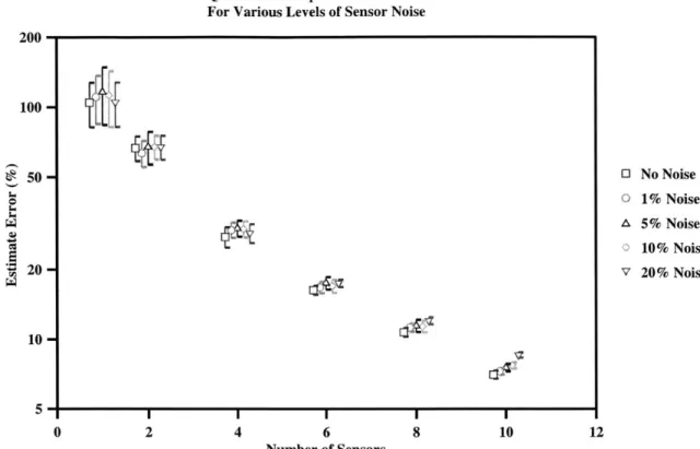
Quasi Static Shape Estimation Error For Various Levels of Sensor Noise 200 100 50- 0 No Noise o 1%Noise A 5% Noise 10% Noise S20 -V 20% Noise 10-0 2 4 6 8 10 12 Number of Sensors
Figure 3-5: Estimation Error as a function of Sensor Noise and Number of Sensor for Quasi-Static Shape Method
3.3.2
Ideal Model with Sensor Noise
The next step is to add sensor noise to the simulation. The sensor noise was added as a percentage of the of the RMS sensor reading for the root strain gage. The sensor reading for the root strain gage was chosen because it is used in all of the sensor layouts.
The effects of the sensor noise on the Quasi-Static estimate is actually very small. For the cases where there are 1, 2, and 4 sensors the difference between the estimate errors is actually in the noise floor of the simulation. Only for the 10 sensor case is there a statistically clear distinction between errors. In that case the difference is between 7% error for the case without noise and 8.5% for the case where the sensor noise is 20%. The percent errors are shown in Table 3.3.2, and Figure 3-5 shows the estimate error versus the number of sensors for the various levels of noise.
Sensor Number of Sensors Noise 1 2 4 6 8 10 0 % 104.74 67.02 27.69 16.34 10.74 7.02 1 % 110.65 63.70 29.63 16.80 11.26 7.26 5 % 116.22 67.82 30.12 17.52 11.47 7.53 10 % 112.50 67.92 29.92 17.03 11.39 7.71 20 % 105.07 67.79 28.71 17.50 12.06 8.57
Table 3.1: Quasi-Static Estimation Error due to Sensor Noise
cases with a high number of sensors becomes clearer when examining the averaged Fourier transform of the system as shown in Figure 3-6 for the 4 sensor case with 20% error. The low frequency portion of the graph is virtually unchanged from previous, while for the high frequency the noise floor masks the signal. When using a limited number of sensors the effects of aliasing cause a similar disturbance level of error as the sensor noise. For a greater number of sensors, the model tries to predict modes that are partially below the noise floor which causes the addition of errors.
3.3.3
Effects of Modeling Errors
While sensor noise is a large cause of error, it is not the only cause. Inherent in any physical system are structural defects, which a model of the structure does not include. These defects range from statistical variations in the modulus, thickness, and density of the components to misplacement and alignment of sensors, and structure damage which can vary over the lifetime of the structure.
In an attempt to model possible errors to the structure the sensing matrix was randomly changed by a small percentage of the mean sensor reading for that mode. For some entries this means a very small net change, while for sensors that are near a node for a particularly mode, it can cause a sign reversal.
The simulations were performed with 5% modeling error and 20% modeling error. While neither error is that significant, they are on the right order for most appli-cations. Figure 3-7 shows the effects that 5% and 20% modeling error has on the estimate error. The figure includes the correctly modeled system for comparison.
10 2 10 100 10 10-2 10-3 , , , , 100 101 102 103 10 Frequency rad/sec
Figure 3-6: Fourier Transform of Quasi-Static Estimate with 20% sensor noise and 4 sensors
Effects of Modeling Error Quasi Static Estimation Error
200-100 - 50-20 2 4 6 Number of Sensors 8 10 0 No Error A 5% Error 0 20% Error 12
Figure 3-7: Results of Modeling Error on Quasi-Static Shape Estimation Error
The additional of modeling error actually has very little effect on the error resulting from the Quasi-Static method, see Table 3.3.3. The only significant error occurs for the case where there is no sensor noise. Even with low or no sensor noise the errors from modeling only have an effect when the errors from aliasing have been lessened
by having multiple sensors.
Sensor Number of Sensors
Noise 1 2 4 6 8 10
0 % 104.74 67.02 27.69 16.34 10.74 7.02
5 % 99.16 71.07 31.25 17.94 11.55 7.48
20 % 119.27 69.85 31.12 16.84 11.28 7.53
Table 3.2: Quasi-Static Method, Effects of Model Error
10
-5
0
3.4
Quasi-Static Shape Estimate with Temporal
Filter
In an attempt to alleviate the effects of aliasing of high frequencies a temporal filter was added. The filter is a low pass filter whose roll-off frequency is set between the last mode sensed and the first aliased mode. In the simulations the sensor data was filtered, but the same effect can be gained by filtering the output signal.
Unlike the unfiltered Quasi-Static method, the method with filtering has transients that occur at the end points of the data. If included these transients can cause tremendous increase in the level of the error. Since the transients are only a relic of the simulation method the end points were thrown out and the RMS errors were calculated from the central data points only.
The same trials were used for filtered case as for the Quasi-Static case. This allows direct comparison of the two methods and reduces the effects of having a limited sample space.
3.4.1
Ideal Model with no Sensor Errors
For the filtered Quasi-Static case with no modeling errors, or sensor noise the system behaved considerably better than without filtering. For this case the greatest source of errors was due to truncation of the system. While the higher frequency modes contribute significantly less to the overall deflection, they do still contribute.
Figure 3-8, shows the percent error in the estimation as a function of the number of sensors. The error is proportional to 1/n2. There is a slight deviation for the eight sensor case, however. This is most likely because the sensor locations are less advantageously placed for the eight sensor case.
3.4.2
Ideal Model with Sensor Errors
An interesting phenomenon occurs when sensor errors are added to the filtered Quasi-Static estimation. The performance actually decreases with the addition of extra