Dynamic ship assignment problem with uncertain demands

Dynamic Ship Assignment Problem

with Uncertain Demands

by

Yoo Joon Kim

Submitted to the Department of Civil and Environmental Engineering

in partial fulfillment of the requirements for the degree of

Master of Science in Transportation

at the

MASSACHUSETTS INSTITUTE OF TECHNOLOGY

February 2016

E

TN Y

@

2016 Yoo Joon Kim. All rights reserved.

JUN

Signature redacted

A u th o r -....-...

...

Department of Civil and Environme al Engineering

anuary

28, 2016

Signature redacted

C ertified by ...

...

Chistopher G. Caplice

Executive Director, Center for

ansportation

and Logistics

Thesis Supervisor

Signature redacted

A ccepted by ...

...

Heidi Nepf

Donald and Martha Harleman Professor of

Ci

il and Environmental

Engineering

Chair, Graduate Program Committee

The author hereby grants to MIT permission to reproduce and to

distribuie _{publicdy paper and electronic copies of this thesis docums'}

Dynamic Ship Assignment Problem

with Uncertain Demands

by

Yoo Joon Kim

Submitted to the Department of Civil and Environmental Engineering on January 28, 2016, in partial fulfillment of the

requirements for the degree of Master of Science in Transportation

Abstract

Product tanker shipping companies in the spot market face severe volatility in demand and in price. We explore shipping companies' two problems: evaluating supply and demand of the market and assigning cargoes in order to maximize profitability. By approximating the market as a queueing system, we obtain utilization ratios, which effectively model supply and demand of the market. This approach directly evaluates the impact of ton-mile on utilization ratios, even a small growth of which may result in a significant supply shortage. Queueing approximation also allows formulation of dynamic ship assignment as a semi-Markov average cost problem, attaining stationary policies. When profit margins are low, a stationary policy frequently rejects cargoes. Despite rejections, it yields the highest profit per cargo, compared to other methods. Such optimal controls remain valid even when demand fluctuates.

Thesis Supervisor: Christopher G. Caplice

Title: Executive Director, Center for Transportation and Logistics

Acknowledgments

This study would not be possible without the help of the following persons: Dr. Chris Caplice, for his invaluable advices and insights, Jakob Tolstrup-Moller of Clarksons, for the provision of dataset that has opened the door for this study, Jung Hee Park, for his advices on search algorithms, Hun Lim, for his introduction to the industry for the novice, Peiguang Hu, for his collaboration on our game theory project, Professor Dimitri Bertsekas, for his teachings and advices on dynamic programming, and last but least, Hyo Young and Samuel, for everything.

Contents

1 Introduction 13

1.1 Product tanker market . . . . 13

1.2 Controller . . . . 14 1.3 Controller's Problem . . . . 15 1.4 Data . . . .. . . . . 16 2 Literature Review 19 2.1 Maritime transportation . . . . 19 2.2 Dynamic programming . . . . 20 2.3 Queueing model . . . . 21 2.4 Game theory . . . . 22 2.5 General references . . . . 22

3 Utilization Ratio Analysis 25 3.1 Definition . . . . 25

3.2 Example . . . . 26

3.3 Assumptions . . . . 26

3.4 Formulation . . . . 27

3.5 Validation . . . . 30

3.6 Application to the real market . . . . 32

3.6.1 Sensitivity . . . . 32

3.6.2 Ton-mile . . . . 33

3.7 Deadline . . . . 34 7

3.8 Utilization ratio game . . . .

3.8.1 Individual ships as players . . . .

3.8.2 Controllers as players . . . .

4 Dynamic Ship Assignment

4.1 Example . . . ..

4.1.1 Assumptions . . . . 4.1.2 Mean service time. . . 4.2 Formulation . . . . 4.2.1 State definitions . . . . 4.2.2 Controls . . . . 4.2.3 Bellman equation . . . 4.2.4 Limitation of queueing 4.2.5 Value iteration . . . . 4.2.6 Stationary policy . . . 4.3 Simulation . . . . 4.3.1 Simulation setting . . . 4.3.2 4.3.3

Simulation over differe Assignment methods 42 43 43 44 45 45 51 51 52 53 53 54 54 approximation it values . . . 4.3.4 Simulation result . . . .

5 Conclusions and Future Research

5.1 Summary . . . .

5.1.1 Susceptibility to utilization ratio 5.1.2 Economy of scale . . . .

5.1.3 Optimal controls with rejections

5.2 Areas for future research . . . .

A Strategy Iteration 8 36 36 37 41 41 56 changes 61 61 61 62 63 63 65

List of Figures

1-1 Histogram by number of loads carried . . . . . 1-2 S Korea to Singapore . . . . 1-3 WC India to Japan . . . . 3-1 3-2 3-3 3-4 3-5 3-6 3-7 3-8 3-9

Example with four ports and two cargo routes Pmf of service times . . . . Exponential distribution . . . . Histogram of simulation result . . . . Waiting time in queue . . . . Laden voyage routes . . . . Ballast voyage routes . . . . Utilization ratio in simulation . . . . Nash equilibria . . . . 4-1 Region with six ports and twelve cargo routes . . 4-2 Demand generated according to Bernoulli process 4-3 Number of rejection states as % of total states . . 4-4 Simulation result, p = 0.08 . . . . 4-5 Simulation result, p = 0.06 . . . . 4-6 Simulation result, p = 0.04 . . . . 4-7 Simulation result, p = 0.02 . . . .

5-1 Sensitivity to utilization ratio . . . .

5-2 Singapore-Japan route . . . . with rate 9 . . . . 17 18 18 . . . . 27 . . . . 30 . . . . 30 . . . . 31 . . . . 32 . . . . 33 . . . . 33 . . . . 35 . . . . 40 p. 42 54 56 57 58 59 59 62 62

5-3 Annual profit per cargo, p = 0.06 . . . . 64

List of Tables

1.1 Clarkson's data . . . . 16

1.2 Transactions by cargo type . . . .. 17

1.3 Top ten routes. . . . . 18

3.1 Nash equilibria . . . . 39

4.1 Stationary policy (p = 0.06, b = 100/day, c = 60/day) . . . . 53

4.2 Queueing analysis . . . . 54

Chapter 1

Introduction

We introduce the product tanker market with a focus on the spot market. Trans-portation demand in the spot market is inherently uncertain and ships constantly face idling time and empty voyages. We also introduce the controller who allocates shipments and we address its problems: evaluating the utilization ratio of ships in a region and assigning cargoes' in order to maximize profitability. Finally, we observe in the market data that cargo arrivals in this market follow Poisson processes.

1.1

Product tanker market

Oil refineries produce various types of petroleum products, which are sold to buyers everywhere according to demand and market price. The distance between produc-tion and consumpproduc-tion drives the global trade of petroleum products, as exemplified

by a large annual volume of naphtha trade from the Middle East to Northeastern

Asia. Geographical arbitrage is another key driver. Traders create demand for ocean transportation when there is a large gap in the price of the same product between two regions. Naphtha, gas oil and fuel oil are the three major products subject to arbitrage trade. Of the 45 million barrels of petroleum products consumed per day globally, almost half (21 million) are traded by sea (Clarkson, 2014). Such seaborne trade is most commonly carried by handysize product tankers with 30,000-40,000 ton

1

"Cargo", "load", and "shipload" are used interchangeably in this thesis.

cargo capacity, also known as medium range (MR) tankers. Product tankers provide so called pickup and delivery service whenever there is a demand (it is called loading

and discharging in the maritime industry).

The product tanker market experiences severe volatility because transportation demand is driven by demand for different petroleum products, which is constantly changing in different regions. Due to such uncertainty, shippers (cargo owners) and shipping companies (carriers) usually do not commit to long-term contracts. Instead, a large number (exact figure unknown) of cargoes are transacted in the spot market based on loosely binding contracts for each cargo which can be canceled without penalty if the ship becomes unavailable. MR tankers are standardized, so petroleum products are moved by similar cargo size and at similar speed. Hence, a ship rarely has any competitive advantage over other ships and is a price taker who carries cargo at market price, which is highly volatile. The product tanker market is highly fragmented and players with differently sizes (mostly small) compete fiercely.

Since petroleum products are liquid and ships are mostly fully loaded with the cargo by a single shipper, cargo is differentiated only by the loading and discharging ports, pickup deadline and charter hire (price), not by types of cargoes. A ship's status is always defined as either laden (fully loaded) voyage or ballast (empty) voyage when sailing.

1.2

Controller

In addition to providing transportation services in the spot market, product tanker shipping companies also carry cargoes on long-term contracts (longer than a single contract) and charter out (lease) ships for a certain period to lock in earnings. This paper deals only with the spot market and we call a tanker shipping company in this context a "controller." The controller is the one who manages a fleet of ships and assigns each cargo to one of the available ships. We call each cargo-ship assignment decision "control." In the real market, a controller may be an individual shipowner, or a corporate entity that manages owned and chartered ships, or a pool operator

who is consigned a number of ships from various shipowners and runs these ships as one pool. Typical large controllers have dozens of ships in their fleets (Lim, 2015).

1.3

Controller's Problem

Due to uncertainty in both demand and charter hire, controllers always try to evaluate supply and demand of the market. Sound evaluation is critical for positioning ships in the right regions for a given period or for planning fleet management (such as investing in new ships) for a longer term. This task is typically done in practice

by comparing the overall growth in tonnage (or the number of ships) in the market

with growth in global petroleum product trade in volume (barrels) (Clarkson, 2014). This paper provides an alternative method by modeling the market as a queueing system. This approach is effective especially when evaluating the impact of a change in ton-mile or a demand change in a specific route, instead of changes in the overall market.

Since significant gaps in profitability between regions are endemic in tanker ship-ping, controllers continually review the optimal allocation (or distribution) of their ships. We formulate this allocation problem as a utilization ratio game and compare the behaviors of controllers with different fleet sizes.

The controller manages several ships in a region and efficiently assigns available ships to irregularly arriving cargoes with an objective of maximizing profit over time. Based on the assignments decisions (or controls), the ships repeat laden voyages, ballast voyages and idling time over specific time periods. Ballast voyage and idling time are the largest costs for a controller, usually much greater than operating costs such as fuel and crew. In practice, such assignments are mostly done manually by a team of chartering managers (Lim, 2015). We formulate this assignment problem as a Semi-Markov problem, obtaining an optimal stationary policy, which maximizes average profit by rejecting some cargoes based on the location and status of ships.

Column name Date Name Built Dwt Hull Type Quantity Type Charterer Laycan From Laycan To Load Discharge Rate Owner data Note Table 1.1: Clarkson's Description

Date of contract or report Ship's name

Ship's built year

Ship's deadweight tonnage Double hull, double sides, etc. Cargo quantity

Cargo type

Shipper or Shipping company 'pick up from' date

'pick up to' date Loading port

Discharging port Freight rate (or price) Shipowner's name

1.4 Data

We provide preliminary analysis of market data in order to illustrate the product tanker market. The dataset, provided by Clarksons, contains 17,097 spot transactions in the handysize product tanker market during January 1, 2011 - October 31, 2014. Handysize tanker refers to ships with the deadweight of 40,000 to 60,000 tons and with the actual cargo capacity of 30,000 to 40,000 tons. The data columns are shown

in Table 1.1.

We don't know how completely the dataset represents the entire spot market transactions during the same period. A significant portion of the transactions are not reported because some transactions are done privately between shippers and controllers, or shipping companies choose not to disclose transaction details as they are conventionally reluctant to reveal their ship positions and status (Lim, 2015). The data shows that a total of 1,542 ships are owned by 344 different owners (each owner owns fewer than 5 ships on average).

Figure 1-1 is a histogram of the number of ships based on the average number of loads carried per year. A ship typically can carry at least one load in a month or twelve cargoes in a year (Lim, 2015). The data shows that only 14% of the ships

16

40,000-50,000 tons Mostly double hull 30,000-40,000 tons

UMS, diesel, Gasoil, etc.

Shell, Total, BP, etc.

5 10 No of trips per year

15

Figure 1-1: Histogram by number of loads carried

Table 1.2: Transactions by

Type No. of

UMS (unleaded motor gasoline)

Gasoil Naphtha Jet

Ultra Low Sulfur Diesel Diesel Oil

Condensate Others

Type not reported Total cargo type transactions % 5,272 2,756 2,366 1,072 641 155 133 92 4,610 17,097

carried five or more loads per year on average. We cannot conclude this due to the incompleteness of the dataset but such figure implies overall low utilization of ships in the market.

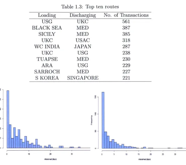
Table 1.2 shows cargo types in the data ordered by the number of transactions. Table 1.3 shows the top ten routes ranked by the number of transactions, which comprise 18% of the entire transactions. The route from the US Gulf region to the UK/Continent region (the Northern European continent plus the UK) had the highest volume, followed by the route from the Black Sea region to the Mediterranean market. In the data, there are a total of 2,123 cargo routes for fewer than 400 ports, implying

17 0 20 of total 31% 16% 14% 6% 4% 1% 1% 1% 27% 100% C: 2? LL C) C3

Table 1.3: Top ten routes

Loading Discharging No. of Transactions

USG UKC 561

BLACK SEA MED 387

SICILY MED 385 UKC USAC 318 WC INDIA JAPAN 287 UKC USG 238 TUAPSE MED 230 ARA USG 229 SARROCH MED 227 S KOREA SINGAPORE 221

R

Figure 1-2: S Korea to Singapore Figure 1-3: WC India to Japan

that the product tanker market forms a very sparse graph. Such sparsity indicates potential long empty voyages.

Figures 1-2 and 1-3 show the histograms of cargo interarrival times for the two busiest routes in the Asian market. As the charts show, interarrival times look to be exponentially distributed. The other major routes also produced a similar pattern. Based on this observation, we assume that cargo arrivals in the product tanker market follow Poisson processes. Such assumption provides a basis for our view of analyzing the market as a queueing system.

18

3-5

3-F

Chapter 2

Literature Review

2.1

Maritime transportation

Christiansen et al. (2004, 2013) reviewed current and past research related to maritime transportation and noted that it mostly deals with optimization problems in a static setting (static as opposed to dynamic or stochastic). Accordingly, mathematical programming (linear, integer or mixed) techniques are the main methodologies. This tendency can be attributed to the characteristics of the specific markets to which those research methods have been applied. In the survey of research papers of the past ten years, Christiansen et al. (2013) divided past research by industry, into liner shipping and tramp shipping.

In liner shipping, carriers, such as container shipping companies, run a regular service between fixed ports and on a published, fixed time schedule, which seldom changes. Hence, problems related to long-term planning (months or up to a year) are the dominant subject in this area. Specifically, network design and fleet deployment problems are the frequent subjects.

In tramp shipping, carriers are plying between different ports, depending on where they find suitable cargoes. The product tanker market, the subject of this thesis, falls under this category. Past research on this market has dealt with fleet size and composition problems. These are the problems of shipping companies that manage ships of various types and sizes and optimize their fleets over the long term by buying

and selling ships or by chartering in and chartering out ships. Another frequent topic of research on tramp shipping is routing and scheduling problems. These types of problems arise when ships have to pick up and deliver cargoes within specific time windows. In this context, the tramp carrier typically has a set of mandatory cargoes, and will try to increase its revenue by transporting optional spot cargoes. The mandatory cargoes are based on agreements between the shipping company and the cargo owners. The key assumption (constraint) in this problem is that ships must carry all those mandatory cargoes, which distinguishes them from our research. We deal with the problems in the spot market, where product tanker companies carry spot cargoes with pickup deadlines based on short-term contracts1. If cargoes are not picked up by the deadlines, the contracts are cancelled without penalty.

The focus of the current research on the liner and contract-based tramp shipping markets is justified, given the size of those markets. According to Gorton et al. (2004),

70% of global goods are carried by non-liner shipping, of which only 5-10% is carried

in the spot market. In this respect, product tanker shipping is a very specialized market, of which spot transactions constitute a large portion.

To summarize, unlike the mainstream of maritime research, this thesis studies the dynamic ship assignment problem with the assumptions that shipping companies have identical ships and have no long-term contracts. To the best of our knowledge, there are no published papers about the dynamic ship assignment problem in the maritime transportation industry.

2.2

Dynamic programming

Product tanker shipping resembles the truckload transportation market in the sense that loads of the same size (shiploads for tankers and truckloads for trucks) arrive with geographical and temporal uncertainty. Like tankers, truckload carriers transport a single shipper's cargo each time. Since demand is uncertain, a dynamic vehicle assignment problem arises - a truck dispatcher manages a fleet of trucks and assigns

'Contracts for spot cargo in tanker shipping are called "voyage charter contracts."

trucks to arriving loads with uncertainty.

The dynamic (or real-time) vehicle assignment problem in the truckload industry has been investigated by Powell (1987, 1986) and Godfrey and Powell (2002). In addition, it has been reported that working vehicle assignment solutions have been developed and implemented in the real market, improving profitability for large truck dispatchers according to Powell et al. (1988) and Simdo et al. (2010).

In formulating the dynamic fleet management2 problem, Godfrey and Powell (2002) approximated cost (or cost-to-go) functions with nonlinear (piecewise linear) functions. With such an approximation structure, cost functions are obtained by computer simulation. Such simulation-based dynamic programming is called approx-imate dynamic programming. In this thesis, we approxapprox-imate the problem itself3, instead of cost functions. We approximate our dynamic ship assignment problem with a queueing system and formulate the problem as a semi-Markov average cost problem. Hence, our solution is analytical (as opposed to simulation-based), in the sense that it is obtained by solving equations. The formulation and proof for such

semi-Markov problems are provided in Bertsekas (2005).

2.3

Queueing model

Larson and Odoni (2007) introduce the formulation and the application of a spatial queueing model. A multiserver spatial queueing system, in particular, is called a "hypercube model." Urban service systems such as police cars and hospital ambu-lances qualify to be queueing systems because both customer arrivals (e.g., 911 calls) and service times (time from call to response) are random. With the assumption that both customer arrivals and service times are exponentially distributed, the hypercube model has been applied to police-sector design, response-area design for ambulances, demand-responsive delivery (pizza), and so on. Since the objective was to compute the workload of each vehicle in the assigned region, vehicles in Larson and Odoni

2_{Not to be confused with the long-term fleet management problem in Christiansen et al. (2013).}

30ften called "problem approximation."

(2007) have identifications and are not anonymous. The anonymity of ships in this

thesis is the key difference, making our formulation much simpler.

2.4

Game theory

Solving Nash equilibria in multiplayer games is an area of computer science. Daskalakis and Papadimitriou (2015) studied anonymous games from an algorithmic viewpoint.

A general n-player game, in which each player has ;> 2 strategies, is described in nC'

numbers, an astronomical number for a large n. For such cases, a Nash equilibrium is not solvable. Anonymous multiplayer games, however, are polynomial in n for fixed .

Daskalakis and Papadimitriou (2015) introduce formulations and algorithms for such games and show that approximate mixed Nash equilibria in anonymous games can be computed in polynomial time. Their paper suggested to the present author that the formulation for our multi-ship or multi-controller game should take the form of dynamic programming. Solutions for both Bellman equations in dynamic program-ming and Nash equilibrium are the fixed points in a given space. We have solved Nash equilibria by what we call "strategy iteration," borrowing the name from "policy iteration" in dynamic programming.

2.5

General references

This thesis is an application of introductory theories taught in the following four classes at MIT (with textbooks cited in parenthesis): 1) Dynamic Programming and Stochastic Control (Bertsekas, 2005), 2) Applied Probability (Bertsekas and Tsitsiklis, 2002), 3) Logistical and Transportation Planning Methods (Larson and Odoni, 2007) and 4) Games, Decision and Computation. Textbooks and classnotes have been used as general references.

Clarkson (2014) publishes monthly business journals on the tanker shipping mar-ket, which we used as a basic introduction to the market. We also interviewed Lim

(2015), who has over 20 years of experience in tanker and bulk ship chartering, for

industry practice and for in-depth introduction to the market.

Chapter 3

Utilization Ratio Analysis

We evaluate the utilization ratio of the ships in a region in the product tanker market

by approximating the region as a queueing system. This approximation is primarily

based on the assumption that cargo demand at each port in the region follows in-dependent Poisson processes. We interpret utilization ratio in two ways, first as an indicator of supply and demand of the market and second as an optimization measure for the controller. We validate the formulation by simulations and discuss applica-tions and limitaapplica-tions of our queuing model. Finally, we formulate the utilization ratio game and compare the behaviors of controllers with different fleet sizes.

3.1

Definition

A utilization ratio (denoted by p) indicates how busy the ships are during a given

period. For example, p of 0.7 indicates that a ship sails (loaded or empty) for 70 out of 100 days while idling for 30 days. By viewing cargo in the region as the customers (or users) and the ships as the servers, our queueing analysis models the region as an

M/M/m queue. M stands for 'memoryless' or exponential distribution for customer

interarrival times or for service times. For our problem, a service means pickup and

delivery of a load. The number of the ships in the region is denoted by m. Utilization

ratio is defined

total rate of cargo arrivals in the region utilization ratio (p) = _{total rate of service}

In this paper, utilization ratio is used in two different contexts with different assumptions about the pick-up deadline. From an analyst's viewpoint, the ratio indicates supply and demand of the market. From a controller's viewpoint, it predicts how the controller's ships are utilized.

3.2

Example

Let us illustrate the formulation using a simple example, in which two identical ships are serving in a region with four ports as shown in Figure 3-1. In this example, we attempt to evaluate supply and demand of the market by calculating the utilization ratio for the region. The solid lines represent laden voyages and the dashed lines represent ballast voyages. Cargoes move over two routes, from port 1 to 2 [route

(1, 2)] and from port 3 to 4 [route (3, 4)]. For route (1, 2), 0.24 shiploads arrive per day on average and for route (3,4), 0.16 shiploads arrive per day. As an example of a service, if a ship idles at port 4 when it is assigned to a load for route (1, 2), the ship must sail empty (ballast voyage) from port 4 to 1 and then sail loaded (laden voyage) from port 1 to 2. Hence, ballast voyage plus laden voyage constitutes one service and it takes 5 days. The ships are assigned to cargoes randomly, i.e., either available ship can be assigned to a load. Under such random assignment, it makes no difference whether the two ships are managed by a single controller or managed by two competitive controllers.

3.3

Assumptions

In order to approximate this region as a queueing system, we need the following assumptions: Cargo arrives according to an independent Poisson process. Sailing time between any two ports is deterministic. Loading and unloading are done in no

1 . - - 3 days 4 \ 2 days 1 day , A1 2=0.24 \ A34=0. 16 - ' 3 1.5 days 2

Figure 3-1: Example with four ports and two cargo routes

time and take zero days. Ships idle only at the discharging ports (port 2 and 4 in the example) and sail only when they are assigned to a load. Ships are anonymous and any ship available can be assigned to any load. Cargo has no pickup deadlines and unassigned loads enter a queue and then are served in a first-in, first-out (FIFO) manner. Service time for a load consists of ballast voyage and laden voyage and is a random variable because ballast voyage is uncertain. We assume it is exponentially distributed.

It is notable that there are two strong assumptions. The first one is related to ser-vice time distribution. Given the assumption that sailing time between any two ports is deterministic, service time is distributed by some probability mass function. How-ever, for a queueing system approximation, we assume that service times of the ships are independently and identically (exponentially) distributed. The second assump-tion is related to the pickup deadline. In the real market, cargoes should typically be picked up by a certain deadline (cancellation date). However, since we intend to evaluate supply and demand of the region, we assume there is no deadline in this example. In other words, there is an infinite queue and cargoes are not lost even if there are no available ships.

3.4

Formulation

In order to formulate the queueing problem we introduce the following notation. The indices i,

j,

27

R set of cargo routes (i, j) in the region

D set of discharging ports in the region

1(j) set of loading ports for shiploads discharged at port j

Ai, Poisson arrival rate for shiploads from port i to j

A total cargo arrival rate in the region

P rate of service of a ship, i.e., picking up and transporting a shipload

p utilization ratio

S sailing (or service) time of a ship

Tij (deterministic) sailing time from port i to

j

7ri (steady-state) probability of a ship idling at port j

Pij (steady-state) probability of a ship serving a shipload from port i to port

j

by A), or total rate of cargo arrivals in the region, is the sum of all arrival rates, i.e.,

A =

(i'j)c

If the ships are randomly assigned to loads, which arrive according to independent

Poisson processes, the probability that a ship is idling at port j while available for assignment in the long run is

Irj = ' for all j in D. A

This is due to the memoryless property of exponential distribution and can be shown by calculating steady-state Markov chain probability.

Hence, the mean service time for serving a shipload from port s to port t is

TSt +

:

where T,, and Tj,, are the deterministic sailing times between ports s and t and between ports

j

Due to the memoryless property of exponential distribution, the probability that

a ship is serving a load from port s to t in a steady state is

Ps't = 't for all (s, t) in 'R.

X

Hence, the mean service time becomes

EF[S] =

Z

S:

- E Ps,tTs,t + I: EP8 ,tljTj,s

(3.4.2)

(8't)ER (s,t)EIZ jEE)

= laden voyage + ballast voyage.

As (3.4.2) shows, mean service time is the sum of the mean laden voyage time and the mean ballast voyage time.

As previously stated in Section 3.3, we purposely assume that service times are independently and exponentially distributed. Hence, the rate for the exponential distribution (denoted by p) is the reciprocal of this mean service time, i.e., P = 1/E[S].

Finally, the utilization ratio is

p = = AE[S] (3.4.3)

ny n

where n is the number of the ships in the region. Since the mean service time E[S] is the sum of laden voyage and ballast voyage, we can rewrite (3.4.3) as

P = PL + PB

where PL is the laden voyage ratio and PB is the ballast voyage ratio, and by the definition of the utilization ratio, we have

PI+ PL + PB = 1

where p, is the idle time ratio. Laden voyage, ballast voyage and idle time ratios indicate how much time a ship spends in sailing loaded, sailing empty and idling,

0.36 0.24 0.24 0.16 1 2 3 4 5 service time 0.4 -0.35 0.3 0.25 0.2 0.15 0.1 0.05 0

Figure 3-2: Pmf of service times

1

I 2 3 4 5

service time

Figure 3-3: Exponential distribution

respectively, during a given period.

3.5

Validation

Applying (3.4.2) to our example in Figure 3-1, we obtain the mean service time by

Al2 A34 A12 A12A34 A34

E[S] _A 1 ' TI,2 + _A 73,4 _+A2T2 + , - ' _A2 ' (T2,3 + 4,1) + _A2 T4,3. (3.5.1)

With A = A,2 + A3,4, we can rewrite the mean service time in (3.5.1) as

2 A,2A3,4 _{A12A, 4 A}

3 4

(Ti,2 + 72,1) + (I,2 + T4,1) + (73,4 + T2,3) A + (T3,4 + T4,3) ' . (3.5.2)

The first two terms in (3.5.2) represent the mean service time of serving shiploads from port 1 to 2. The remaining two terms represent the mean service time of serving shiploads from port 3 to 4. When a load arrives at the region while there is an available ship (or ships), the ship is randomly located either at port 2 or at port 4. The fractional terms in (3.5.2) correspond to the probability of each event in the probabilistic sample space. For example, the fraction in the first term, A ,2/A 2,

represents the probability of an event that a ship is located at port 2 when it is assigned to a load from port I to 2, in which case, the service time is 4 days (= T1,2 +T 2,1). The

probability mass function of service times (S) for the example is shown in Figure 3-2. Given the probability distribution, the mean service time for the example equals

30

0.4

0.3

0.2

700 600 600 5o 500 > 400 - -400 300 300 200 200 100 100 0 0 3.4 3.45 3.5 3.55 3.6 3.65 0.6 0.65 J./ 0.75 0 S 0.85

mean service tine utilization ratio

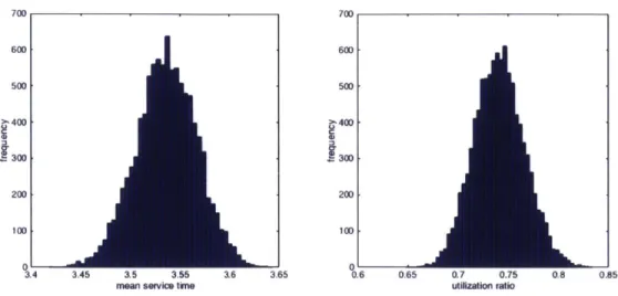
Figure 3-4: Histogram of simulation result

3.56, i.e., it takes 3.56 days on average for the ships to transport a load in this region.

The utilization ratio computes to 0.712, i.e., the ships are busy (sailing) during 71% of the time.

We ran a simulation for 10,000 times to test the formulation and plot a histogram of the result as shown in Figure 3-4. Each simulation generated 1,000 cargoes accord-ing to the arrival rates and assigned the ships randomly. The mean service time in the simulation is 3.54 days and the utilization ratio is 0.741. While our estimate for the mean service time is close to the simulation result, the histogram shows that our model has a high probability to underestimate the utilization ratio. In other words, the ships in the simulation were busier than expected. Such gap between estimation and simulation result is obviously because we assume that service times follow expo-nential distribution, which is different from the probability mass function shown in Figure 3-2. In the pmf, the probability of service time being longer than the average is higher than the probability of being shorter than the average. Our exponential distribution would assume the opposite (see Figure 3-3).

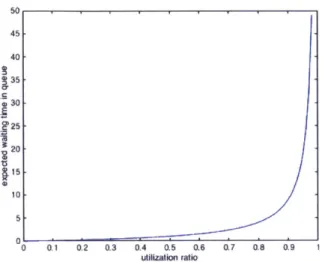
50 45 40 35 D 30 0'25 20 15 10 01 0 0.1 0.2 0.3 0.4 0.5 0.6 0.7 0.8 0.9 1 utilization ratio

Figure 3-5: Waiting time in queue

3.6

Application to the real market

3.6.1 Sensitivity

We claim that utilization ratio analysis can be used for evaluating supply and demand of the market. Can a specific utilization ratio indicate whether the market is oversup-plied or not? The answer can be obtained when the model is apoversup-plied and tested using the real market data, which is beyond the scope of this paper, but queueing theory helps us to understand that the tanker market becomes highly sensitive to changes in

demand when levels of utilization are high. Figure 3-51 illustrates this phenomenon that the expected waiting time in queue for a user (cargo) grows exponentially as the utilization ratio becomes close to 1. Waiting time represents the delay between the time a cargo arrives at the market and when it is actually picked up. Hence, a very long waiting time means the market suffers a severe shortage of ships. In such a case, our queueing model shows that the market (price) will fluctuate even with a small change in demand.

'For an M/M/1 queue with p 1.

Figure 3-6: Laden voyage routes Figure 3-7: Ballast voyage routes

3.6.2 Ton-mile

The tanker market participants view ton-mile, one ton of cargo carried one nautical mile, as an important driver of demand. Increase in ton-mile is typically understood as growth in cargo volume for long-haul routes or emergence of new cargo routes that increase overall sailing time and distance. From the queuing model point of view, a change in ton-mile can be interpreted as a change in service time (or utilization ratio), thus our model can directly estimate the impact of change in ton-mile.

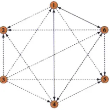
To illustrate this idea, we introduce another example as shown in Figure 3-6 and in Figure 3-7. There are six ports and twelve cargo routes in the region. The sailing time between ports is two, three, or four days. For example, it takes two days for route (1, 2), three days for route (1, 3), and four days for route (1, 4). There are three identical ships in the region. Cargo arrivals for each cargo route follow the identical distribution (Poisson) with the rate (denoted by p) of 0.04 shiploads per day. Hence, the total arrival rate (A) is 0.48, i.e., a new shipload arrives at the market every

2.08 days. Based on the same assumption stated in Section 3.3, the utilization ratio

computes to 0.898. Hence, as shown in Figure 3-5, the market is highly sensitive to even a small change in the utilization ratio. The laden voyage ratio equals 0.44 and the ballast voyage ratio equals 0.458.

Now suppose the overall demand (A) in the market increases by 1.0%. But the rates of change are not uniform over different routes. The demand for routes (1, 4) and (4, 1), the long-haul cargoes, increases by 18.5% while the demand for routes (1, 6),

(3, 4), (5, 4), (5, 6) and (6, 1), the short-haul cargoes, decreases by 5.0%, while demand

33

for the remaining routes remain unchanged. Can we expect that the utilization ratio to increase by 1.0% in line with the overall demand growth?

Our queueing model says otherwise. The new utilization ratio equals 0.918, a

2.3% increase and the laden voyage ratio increases by a greater 3.0%. It is because

the growth in long-haul demand not only increased the overall demand but also raised the mean service time. Given the already very high utilization ratio base, we

can expect the change in demand will cause a much worse supply shortage.

3.7

Deadline

In our two previous examples, we assumed an infinite queue capacity. This means that shiploads are not lost even if no ships can pick up the shiploads within deadlines, and instead, they are postponed. Such assumption makes sense when we evaluate supply and demand of the market using the utilization ratio. However, we need to revise the assumption when a controller attempts to evaluate its own utilization ratio in a competitive region. Since there are competitors, cargoes are highly likely to be lost if not picked up within deadlines. Unfortunately, it is impossible to accurately model such situation using queueing theory. One alternative is to model the problem as an

M/M/m/K queue. The capacity of the queueing system is denoted by K.

We use the same region with six ports as shown in Figure 3-6 and Figure 3-7 as an example to illustrate this modeling issue. The controller manages three identical ships in the region and wants to evaluate the utilization ratio of its ships. We assume that all cargoes have a deadline of 4 days. If no ships are available within the deadline, cargoes are lost. We attempt to model this problem as an M/M/3/3 queue. This means the queuing capacity is zero and cargoes are lost immediately when no ships are available. All the other assumptions stated in 3.3 remain valid for this problem.

Since cargoes are lost when all of the three ships are busy, we need to calculate the probability of such event (denoted by Pm) by Erlang's loss formula (Larson and Odoni, 2007)

(A/p)m/n!

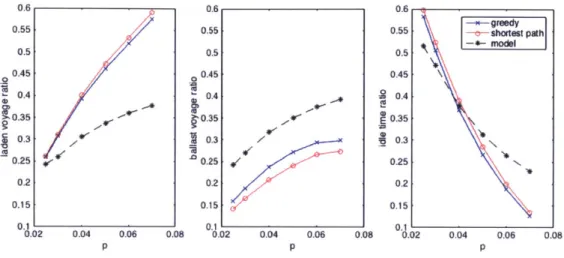
0.6 0.55 0.5 0.45 0.4 >0.35 50.3 0 .25 0.2 0.15 0.1 0.02 0.04 0.06 0.08 0.6 0.55 0.5 0 0.45 0.4 0.35 0.3 0.25 0.2 0.15 0.1 0.02 0.04 0.06 0.08 0.6 greedy 0.55 _{shortest path} 0.5 -+- model 0.45 \ 0.4 0.35 0.3 0.25 0.2 0.15 0.1 0.02 0.04 0.06 0.08

Figure 3-8: Utilization ratio in simulation

Total demand in the region is now A(1 - Pm). Therefore, the utilization ratio is

A(1 - Pm) ny

We test the formulation by simulation. In this simulation, time is discretized and it advances in one day intervals. Shiploads for each route are generated at each time interval according to Bernoulli process (as a discrete version of Poisson) with a success rate of p and are cancelled if they are not picked up by an available ship by the deadline. The duration of each simulation is 365 days and we repeat it for 100 times. Simulations are done for different values of arrival rate p. We use two assignment methods for each cargo in the simulation, 'greedy assignment' and 'shortest path algorithm.' The greedy method immediately assigns the closest available ship to a cargo, which is similar to the random assignment assumption that we use to calculate the utilization ratio. We will explain these methods in detail in Section 4.3.3.

The result in Figure 3-8 shows that our model significantly underestimates the laden voyage ratio while overestimating the ballast voyage ratio. The reason for the error is that our model excludes the possibility of not immediately assigned shiploads being picked up by the ships that become available within the four-day deadline. This explains why the error for the laden voyage ratio is greater for high values of p.

3.8

Utilization ratio game

So far we have evaluated utilization ratio for a single region. Now imagine a market divided into several regions where multiple controllers are competing. Ships can move between regions (freely or for a cost) and controllers distribute their ships over different regions with an objective of maximizing utilization ratios. We view this game from two different perspectives, depending on how we define a player. In the first perspective, the players are individual ships that choose a region to maximize the utilization ratio. In the second perspective, the players are individual controllers who have one or more ships and maximize the average utilization ratio.

For analysis of this anonymous, multiplayer game, we assume a complete infor-mation setting2

3.8.1

Individual ships as players

In this market, there are n ships and regions and ships can move freely between regions. We define demand-service ratio, denoted by 1, a ratio of total demand rate

(A,) and total service rates (pi) for region 1. It corresponds to utilization ratio if there is only one ship in the region. The higher the ratio is, the more ships are demanded. We also introduce the following notation:

#i

[n] set of players, [n] = {1, 2, ... , n}

[]

[1]

{1,

}

A set of distribution over

[(]

6 mixed strategy profile

6i mixed strategy of player i in 6

6-i collection of mixed strategies except for i's in 6

6i (1) probability of player i being positioned in region 1 E

[]

Pure strategy (action) of a player (ship) in this game corresponds to the region

2

1n a complete information game, the number of players, a finite set of pure strategies for each player, and a utility function of each player are known to all players.

in which the ship is positioned. Each player uses a randomized (or mixed) strategy (denoted by 6j), i.e., a strategy takes the form of a distribution over [i]. For example,

6i(1) means the probability of player i being positioned in region 1. Mixed strategy

profile (denoted by 6) is the collection of strategies of all players, i.e., it is a mapping of [n] onto Y. Since any ship can go to any region in the market, all players have the same strategy set.

Utility of player i when positioned in region 1 is calculated as

U = _{1 nj} A , for all i E [n] (3.8.1)

+1

where ni is the number of players except for player i choosing strategy 1. Since all players have the same strategy set

[]

and nj becomes a binomial random variable.

Finally, from the fact that all players share the same mixed strategy, the Nash equilibrium simply is

6* (l) = , for all i E [n].

The Nash equilibrium suggests that positioning a ship following the distribution of demand (or 3) is the best response of any player. This obvious result explains 'herd mentality'; a rational player should do exactly what other players do - positioning more ships in the market with more demand - and unilaterally deviating from this strategy will only deteriorate its payoff.

3.8.2

Controllers as players

In this section, controllers who have multiple ships are the players. Since different players have different pure strategy sets depending on the number of ships they con-trol, the game is no longer symmetric. We discuss such games using a simple example

where 100 'small' players who have only one ship each compete with a single 'big' player who has 100 ships. The market consists of two regions, namely region 1 and

re-gion 2. The demand-service ratios for each market, pl and 2, are given as parameters. For this example, we assume that there is a fixed cost for switching regions.

We introduce the following notation:

B set of pure strategies of big player, i.e., bj E B

bj pure strategy of big player,

j

b' number of big player's ships in region 1

C

{1,

[

6i mixed strategy of small player i E {0, 1, 2, ..., 100}

ZJ probability of small player i being in region 1

A specific pure strategy of the big player is denoted by bj = (b!, b ) where b and

b? represent the number of ships in region 1 and region 2, respectively. The big player

has 101 pure strategies, i.e., B {(0, 100), (1, 99), (2, 98), ... , (100, 0)}. Small players have two pure strategies, i.e.,

[ ]

{1,

i is denoted by 6=

(6

being in region 1 and region 2, respectively. The big player plays one of the pure strategies and small players play mixed strategies in this game.

We evaluate the Nash equilibrium in the following situation:

" In the initial state, the ship demand in region 1 and region 2 are equal, i.e.,

p(O) =

p

distribute their ships in those two regions, i.e., the big player plays (50, 50) and small players play (0.5,0.5).

" In the new state, the demand in region 1 becomes twice as big as the demand

in region 2, while overall demand remains unchanged. The demand of region 1 and region 2 are now p9 = 120 and 2 = 60, respectively.

We want to find the Nash equilibrium and utilization ratio for each player in the new state. We do this by iteratively searching over the pure strategies of the big player

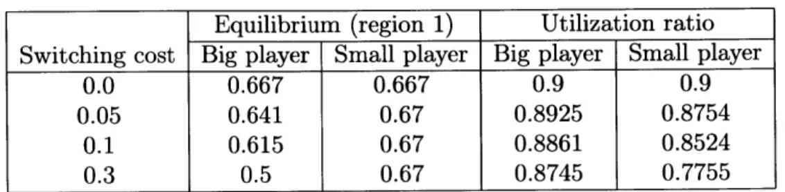
Table 3.1: Nash equilibria

Equilibrium (region 1) Utilization ratio Switching cost Big player Small player Big player Small player

0.0 0.667 0.667 0.9 0.9 0.05 0.641 0.67 0.8925 0.8754

0.1 0.615 0.67 0.8861 0.8524

0.3 0.5 0.67 0.8745 0.7755

and over the mixed strategies of small players (we call this "strategy iteration"). We include the formulation for the strategy iteration in Appendix A.

We obtained Nash equilibria and the corresponding utilization ratios with varying switching cost. The unit of cost is utilization ratio. For example, a switching cost of

0.1 means that switching from one region to another will cost a ship 0.1 utilization

ratio.

As Table 3.1 shows, if there is no switching cost, the equilibrium suggests that both the big player and small players will distribute their ships according to the demand-service ratio distribution (2/3 for region 1 and 1/3 for region 2). The big player will position two-thirds of its ships in region 1, and small players will position its ship to region 1 with a probability of 0.667. Hence, the utility of the big player and small players are the same.

As switching cost increases, big player's allocation to region 1 does not increase as much as the demand grows. Eventually, when switching cost is greater than 0.3, the big player stays in its initial distribution (50, 50). On the other hand, small players will always distribute their ships according to the demand distribution. As a result, the utilization ratio of small players sharply decreases as the switching cost grows while the average utilization ratio of the big player remains high (see Figure 3-9).

The result reveals that a large controller who operates a number of ships will react to a change in demand more conservatively than smaller players. In other words, the large controller causes a shortage in ships by not supplying enough ships to the regions with high demand. Small controllers, in contrast, will distribute their ships according to the distribution of market demand. As a result, the large player obtains greater utilization ratio. It may be counter-intuitive to find that the Nash equilibrium in our

0.9 0.8 0.7 E 0.6 0.5 c 0.4 z 0.3 0.2 0.1 01 0 0.1 0.2 0.3 0.4 0. Switching Cost Big pfayer 0.95 -Small play 0.9 0.85 0.8 .2 0.75 0.7 0.65 0.6 0.55 0.5' 5 0 0.1 0.2 0.3 0.4 Switching cost

Figure 3-9: Nash equilibria

example suggests that big player will not aggressively move ships to region 1 (high market) since it has the lower average switching cost per ship compared to that of a small player. However, such strategy makes sense given the fact that it already has exposure (ships) in both regions and thus it does not have to make aggressive allocation changes, which will only incur unnecessary switching cost. In contrast, it is the only option for small players to switch to a better market despite the switching cost because the opportunity cost (cost of not moving) is greater than switching cost.

40

.1

]r

Chapter 4

Dynamic Ship Assignment

In this final problem, a controller assigns ships to irregularly arriving cargoes with the objective of maximizing profit over time. With the assumption that both cargo inter-arrival times and ship service times are exponentially distributed, the tanker market is viewed as a queueing system, and the problem is approximated as a Semi-Markov problem that minimizes average cost (or maximizes average profit) over an infinite horizon. The stationary policy obtained from Bellman equations for the problem suggests cargo rejections, depending on the status and the location of ships. Despite rejections, the stationary policy yields the best profit per load among alternative as-signment methods when profit margins for each load are low. On the contrary, when the margins are high, myopic greedy assignment method yields comparable results. The stationary policy also suggests that the controller needs to be selective even when demand is low in order to maximize profit.

4.1

Example

We use the same example used in Section 3.6.2 - a hypothetical region with six ports - to illustrate this optimal control problem. We also use the same nota-tion introduced in Secnota-tion 3.4 to describe the region in the example and formu-late the mean service time. In Figure 4-1 the solid lines represent laden voyage (cargo) routes and the dashed lines represent ballast voyage (empty voyage) routes

( 2 - - - - - - - ----

( 3 - - - - -- - - - - - 5

4

Figure 4-1: Region with six ports and twelve cargo routes

traversed to pick up cargoes. There is a total of twelve cargo routes, i.e., R=

{(1, 3), (1, 4), (1, 6), (2, 4), (4, 1), (4, 3), (4, 6), (5, 1), (5, 4), (5, 6), (6, 1), (6, 4)}. The

con-troller has three identical ships.

This region forms a graph that has far fewer edges (or cargo routes) than the maximum number of edges (30) for a six-node graph. The real product tanker market also typically forms such sparse graphs and thus ships inevitably experience long ballast voyages. For example, port 3 in Figure 4-1 has only incoming cargoes without backhaul (or outgoing) cargoes, so ships that discharged cargo at port 3 must make a ballast voyage to pick up the next cargo.

4.1.1

Assumptions

Sailing time between any two ports is deterministic. Loading and unloading are done in no time and take zero days. Ships idle only at the discharging ports (D =

{1, 3, 4, 6}) and sail only when they are assigned to a load. Shiploads sailing along

the twelve cargo routes arrive according to independent Poisson processes. Shiploads have pickup deadlines; any shiploads unassigned by those deadlines are lost forever. Time to process a load consists of ballast voyage (cost to the controller) and laden voyage and is distributed by some probability mass function, as ballast voyage is a random variable. However, for a Semi-Markov formulation, it is assumed service

times are independently and exponentially distributed.

While the remaining assumptions are the same as those stated in Section 3.3, there is one important distinction: we assume that service time for each route follows a different exponential distribution. In Section 3.3, we assume that all service times, regardless of the route, follow the same exponential distribution.

4.1.2

Mean service time

Cargoes arrive according to independent Poisson processes. If ships are randomly assigned to a load, the probability that a ship is located at port

j

Ziel(j) Ai j

assignment in the long run is 7rj = '- for all J in D. Hence, the mean service time for serving the load from port s to t is

E[T,,t] = Ts,t + Y3 7rjrj,, for all (s, t) in R?

jE'D

where rs,,t and Tj,, are the deterministic sailing times between ports s and t and

between ports

j

-- 1

reciprocal of this mean service time, i.e., T,,,.

It is worth pointing out that the mean service times for each cargo route need to be calibrated during simulations when we apply different assignment methods since a certain method will change the probability that a ship idles at port

j

4.2

Formulation

We approximate our problem as a semi-Markov problem by assuming that both cargo interarrival times and service times are exponentially distributed. In semi-Markov problems, the time between successive controls (or state transitions) is a continuous random variable and cost is continuously accumulated. For example, in queueing systems state transitions correspond to arrivals or departures of customers. Because

we essentially approximate the tanker market as a queueing system, for our ship assignment problem, state transitions occur when a new load arrives at the region.

We formulate our problem as a semi-Markov average cost problem and obtain a stationary policy by solving the corresponding Bellman equation. In dynamic pro-graming, a policy (denoted by 7r by convention) is a sequence of functions (denoted by

pk) that map states onto controls, i.e., functions that output a control (or decision)

based on a given state. A stationary policy minimizes the average cost per stage over an infinite horizon and contains a function (denoted by p) that outputs an optimal control based on a given state, irrespective of the time of the control. Hence, controls in the stationary policy for our problem assign the ships to a new load based on the given state, minimizing the average cost (or maximizing average profit) over an infi-nite horizon. A state includes the route for a new load and the status and location of the three ships, as explained in the following section.

4.2.1

State definitions

A state is defined as a quadruple of origin-destination pairs (s, t)(si, i)(s2, j)(s3, k)

where (s, t) is an arriving load required to be shipped from port s to t. The (Si, i)(s₂, j) (S3, k) means the three ships are serving cargoes from port si to i, from S2 to j and

from s3 to k, respectively. A ship idling at port i is represented by (0, i). For example,

the state (s, t)(0, i)(0, j)(m, n) means that two ships are idling at ports i and

j

The total number of states is O(IEIN'+) where N is the number of the ships under control. We have total 5,424 states for the problem as ships are anonymous. The state space is finite and forms a single recurrent class.