HAL Id: hal-00317093
https://hal.archives-ouvertes.fr/hal-00317093
Submitted on 1 Jan 2003
HAL is a multi-disciplinary open access
archive for the deposit and dissemination of
sci-entific research documents, whether they are
pub-lished or not. The documents may come from
teaching and research institutions in France or
abroad, or from public or private research centers.
L’archive ouverte pluridisciplinaire HAL, est
destinée au dépôt et à la diffusion de documents
scientifiques de niveau recherche, publiés ou non,
émanant des établissements d’enseignement et de
recherche français ou étrangers, des laboratoires
publics ou privés.
Latitudinal extent of large-scale structures in the solar
wind
H. A. Elliott, D. J. Mccomas, P. Riley
To cite this version:
H. A. Elliott, D. J. Mccomas, P. Riley. Latitudinal extent of large-scale structures in the solar wind.
Annales Geophysicae, European Geosciences Union, 2003, 21 (6), pp.1331-1339. �hal-00317093�
Annales
Geophysicae
Latitudinal extent of large-scale structures in the solar wind
H. A. Elliott1, D. J. McComas1, and P. Riley2
1Southwest Research Institute, San Antonio, Texas, USA
2Science Applications International Corporation,San Diego, California, USA
Received: 20 September 2002 – Revised: 21 February 2003 – Accepted: 25 February 2003
Abstract. Comparison of solar wind observations from the ACE spacecraft, in the ecliptic plane at ∼1 AU, and the Ulys-ses spacecraft as it orbits over the Sun’s poles, provides valu-able information about the latitudinal extent and variation of solar wind structures in the heliosphere. While qualitative comparisons can be made using average properties observed at these two locations, the comparison of specific, individual structures requires a procedure to determine if a given struc-ture has been observed by both spacecraft. We use a 1-D hydrodynamic code to propagate ACE plasma measurements out to the distance of Ulysses and adjust for the differing longitudes of the ACE and Ulysses spacecraft. In addition to comparing the plasma parameters and their characteris-tic profiles, we examine suprathermal electron measurements and magnetic field polarity to help determine if the same fea-tures are encountered at both ACE and Ulysses. The He I λ 1083 nm coronal hole maps are examined to understand the global structure of the Sun during the time of our heliospheric measurements. We find that the same features are frequently observed when both spacecraft are near the ecliptic plane. Stream structures derived from smaller coronal holes during the rising phase of solar cycle 23 persists over 20◦–30◦ in heliolatitude, consistent with their spatial scales back at the Sun.
Key words. Interplanetary physics (solar wind plasma)
1 Introduction
Coronagraph measurements provide information about the size and three-dimensional shape of coronal structures within
∼30 RS of the Sun, but further out in the solar wind, much less is known about how such large-scale structures evolve. Over the past forty years, most of what has been learned about the heliosphere has been based on in-ecliptic measure-ments. In contrast, the unique orbit of Ulysses, which passes over the Sun’s poles, provides in situ measurements as a function of latitude. Ulysses has already greatly enhanced
our knowledge of the 3-D structure of the inner heliosphere during solar minimum when the large-scale structure varies slowly (e.g. McComas et al., 2000, and references therein). For example, Ulysses solar minimum measurements revealed a relatively simple heliospheric structure with high–speed streams emitted from large polar coronal holes filling the high latitude heliosphere. In contrast, near-maximum solar wind is much more complex with highly variable flows aris-ing from a variety of coronal sources observed at all heliolat-itudes (McComas et al., 2002a).
In this paper we have two goals: (1) to develop and test techniques for determining when two spacecraft observe the same large-scale structures, such as coronal hole flows and Coronal Mass Ejections (CMEs) in the heliosphere, and (2) to determine the latitudinal extent of these structures in the heliosphere.
Hydrodynamic codes have been used to study the solar wind for a long time, and simulations have advanced to the point of being 3-dimensional magnetohydrodynamic codes with solar observations supplying inner boundary conditions (e.g. Riley et al., 2002). We use 1-D hydrodynamic simula-tions driven at the inner boundary with spacecraft observa-tions, and adjust the data in time to account for corotation with the Sun. In some Helios (e.g. Schwenn et al., 1981) and Pioneer (e.g. Mitchell et al., 1981) studies, observations from pairs of spacecraft were rotated to align measurements in longitude, but they used a constant solar wind speed for propagation between spacecraft. Very few studies have used a 1-D code with a driven inner boundary. We know of only one other study by De Keyser et al. (2000) that uses such a technique to examine sector boundaries. However, these au-thors limited their study to the rare times when WIND (1 AU) and Ulysses (5 AU) were in radial alignment. Our study is unique in that we use Ulysses and ACE data when the space-craft have latitude separations from 0–42◦, and then use the sector information as a tool to examine the latitude extent of large-scale structures, and their dynamic evolution.
Several other recent studies used different approaches to examine large-scale features. Recently, Neugebauer et al.
1332 H. A. Elliott et al.: Latitudinal extent (2002) compared Ulysses and ACE data to solar
observa-tions to determine the source site on the Sun of the different types of solar wind. We use both ACE and Ulysses data as do Neugebauer et al. (2002), but we focus on the dynam-ics of large-scale structures. Recent work by Riley et al. (2002) provides motivation for examining the dynamics of large-scale features in the inner heliosphere. They found that using constant speed mapping produces a significantly dif-ferent heliospheric current sheet shape than when dynamics are included. Neugebauer et al. (1998) showed that a mag-netohydrodyanmic (MHD) model and several source-surface models predict boundary positions that differ by as much as 20◦. Wang et al. (2000a,b), and Richardson et al. (2002) ex-amined the evolution of structures in the distant heliosphere by comparing Ulysses and Voyager data. We focus our at-tention on the evolution of structures from 1–5 AU, which is a region where stream interactions grow and the coalescence of structures begins to occur. The slowdown of the solar wind by interstellar neutrals is negligible within 5 AU. The region from 1–5 AU is ideal for studying stream evolution and the development of corotating interaction regions
2 Coronal hole plasma and CMEs
High-speed streams have a characteristic speed profile due to compression and rarefaction produced as the streams in-teract with surrounding slower plasma. Plasma emanating from coronal holes has other interplanetary signatures in ad-dition to having high speed. These signatures include the proton to alpha ratio, magnetic field structure, heavy ion composition, and ion charge state abundance. High-speed streams tend to consist of one magnetic polarity. This sup-ports the predominant view that high-speed streams (>700 km s−1) generally come from coronal holes, which also con-sist of one dominant polarity (Hundhausen, 1977). High-speed streams have low oxygen and carbon freezing-in tem-peratures and low Mg/O and Fe/O ratios (Geiss et al., 1995), low density (Belcher and Davis, Jr., 1971), relatively struc-ture free plasma parameters (Feldman et al., 1996, and refer-ences therein), and Alfv´en waves are often present (Belcher and Davis, Jr., 1971). High-speed streams associated with the large polar coronal holes that Ulysses observed around solar minimum, have a mean speed of ∼760 km s−1, mean 1 AU temperature of 2.7 × 10⁵K, mean 1 AU density of 2.7 cm−3, and a mean alpha to proton ratio of 4.4% (McComas
et al., 2000).
Here, we present observations during the rising phase of the solar cycle. Around solar maximum large-scale tran-sient coronal mass ejections are more frequent (Webb and Howard, 1994). While there are many in situ signatures of Interplanetary Coronal Mass Ejections (ICMEs), no one sig-nature can be used to identify all ICMEs (Gosling, 1996; Neugebauer and Goldstein, 1997). Recently, these signa-tures have been reviewed by Gosling (1996, 1997), and Neugebauer and Goldstein (1997). At 1 AU the presence of counterstreaming suprathermal electrons is a fairly reliable
signature of ICMEs (Gosling, 1996). A few other criteria are enhanced helium abundances (He++/H+ >0.08), low beta, strong magnetic fields, and unusual ionization states such as Fe+16.
In addition to changes in the frequency of CMEs with the solar cycle, the number and size of coronal holes vary over the course of the solar cycle. At solar minimum there are two large polar coronal holes and an equatorial streamer belt. However, during the rising phase and near solar maximum the polar coronal holes shrink in size and eventually disap-pear, and many small coronal holes develop (Wang et al., 1996). These small coronal holes are not limited to high lat-itudes and occur at mid and low latlat-itudes. Many of these small holes are associated with active regions and transients (Wang et al., 1996). During the descending phase of the solar cycle, polar coronal holes reform, and equatorial extensions to polar coronal holes are more common (Hundhausen et al., 1981). The lifetimes of coronal holes are greater during the descending phase (Hundhausen et al., 1981). These smaller coronal holes produce streams in the heliosphere with speeds typically reaching only 500–600 km s−1, which is less than the large coronal holes (McComas et al., 2002b). However, McComas et al. (2002b) found the freezing-in temperatures to be characteristic of the larger polar coronal holes. The small coronal hole freezing-in carbon and oxygen tempera-tures were less than 1.1 MK and 1.3 MK, respectively.
3 Data and model
Primarily, we use ion and electron measurements from the Advanced Composition Explorer (ACE) and Ulysses space-craft. These observations are taken from the ACE Solar Wind Electron Proton Alpha Monitor (SWEPAM) (McCo-mas et al., 1998) and the Ulysses Solar Wind Observations Over the Poles of the Sun (SWOOPS) instruments (Bame et al., 1992). Supporting observations from the magne-tometers on Ulysses (Balogh et al., 1992) and ACE (Smith et al., 1998) are also used. During the time of this study, 5 February 1998 to 31 December 1999, the ACE spacecraft was near Earth at L1, and Ulysses started at 2◦latitude and 5.39 AU and went south, ending at −42◦ latitude and 4.16 AU.
To propagate data from 1 AU (ACE) out to the location of Ulysses, we use the Zeus astrophysical single-fluid mag-netohydrodynamic model (Stone and Norman, 1992). The model uses a Eulerian finite difference scheme. Although the Zeus model can include magnetic fields and radiation transport, in this study they are neglected and only hydro-dynamic effects are examined. Not including magnetic fields causes waves to travel at the sound speed instead of the mag-netosonic speed. A further consequence of not including hy-dromagnetic effects is that forces due to magnetic pressure gradients and tension are not included (Riley et al., 1997). Since we examine data at radial distances less than 5.4 AU, pickup ions effects are not included. Inclusion of pickup ions would slightly modify the pressure profile (Riley and
500 1000 1500 2000 2500 So la r W in d S p e e d [ km /s ] Radial Propagation So la r W in d S p e e d [ km /s ] 1.00 AU 1.70 AU 2.40 AU 3.10 AU 3.79 AU 4.49 AU Closest 5.39 AU Ulysses <R>=5.40 AU Ulysses Model ACE 200 400 600 800 S o la r W in d S p e e d [ k m /s ] 0.1 1.0 D e n si ty [ c m -3] 104 105 Te m p e ra tu re [ K ] 1998.25 1998.30 1998.35 1998.40 1998.45 1998.50 M a g n e ti c P o la ri ty Ulysses ACE 1.200 -33.81 -1.00 -51.54 -3.60 -69.24 -6.60 -86.48 -9.60 -103.7 -12.7 -120.8 DLONG DLAT Year Model Ulysses LARP Ulysses Model Model Ulysses 4/1 (91) 4/19 (109) 5/7 (127) 5/26 (146) 6/13 (164) 7/1 (182)
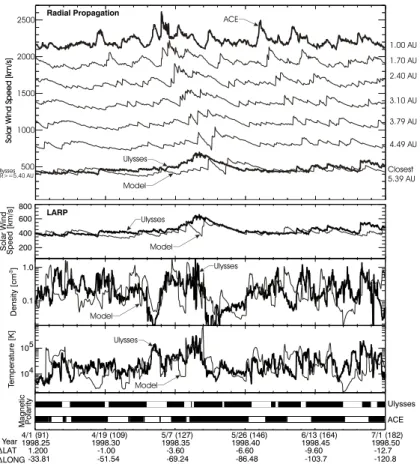
Fig. 1. The top panel shows ACE solar
wind speed data at 1 AU as a thick line, and model speeds at given propagation distances as thin lines. The Ulysses data overlays the ACE propagated data at the grid step that most closely matches the distance of Ulysses. Subsequent pan-els compare Ulysses data and model re-sults when the longitudes of the two spacecraft have been aligned in addition to the radial propagation. The second panel displays the velocity, the third panel the density, the fourth panel the temperature, and the last panel the po-larity of the magnetic field. Additional
x-axis labels indicate the difference in latitude (1LAT) and longitude (1Lon) between the ACE and Ulysses space-craft.
Gosling, 1998). The model solves a system of continuity, momentum, and internal energy equations. A polytropic in-dex of 3/2 is used since most solar wind measurements are generally consistent with this value (Riley et al., 2001). Even though Zeus is a 2-D model, only one dimension is used in this study so that we can use single point in situ measure-ments to drive the model. Since we know the inner boundary conditions (1 AU) for a point, we use a 1-D version of the model to propagate measurements from ACE at 1 AU to the position of Ulysses when it was at distances between 4.2 and 5.4 AU. We focus on the dynamic evolution of structures be-tween 1 and 5.4 AU without making assumptions about the solar wind properties at locations away from our measure-ments. Gosling et al. (1995, 1998) showed that a 1-D model predicts many key features of ICMEs, which are also found in more complex 2-D models of ICMEs (Riley et al., 1997). However, a 1-D model cannot accurately predict complex ef-fects like those observed by Riley et al. (1997) in their 2-D model. Riley et al. (1997) found that latitudinal gradients in the ambient solar wind speed can affect the evolution of an ICME to the extent that an ICME may split in two. A 1-D model would not be able to predict such a split. De Keyser et al. (2000) found that by using a 1-D model they could often identify sector boundaries observed at Ulysses in the WIND data when Ulysses and WIND were in radial alignment.
We use hourly averages of the Ulysses-SWOOPS and ACE-SWEPAM plasma measurements. The ACE measure-ments are used as the inner boundary conditions for each time
step of the simulation and then we compare the propagated ACE measurements with the Ulysses measurements. Since the Ulysses spacecraft position varies slowly around aphe-lion, the data are split into 4 segments per year to calculate an average radial position. For each segment we compare U-lysses SWOOPS measurements to ACE mapped data at the radial grid point that most closely matches the average ra-dial distance of Ulysses. The grid size is 0.47 RS. We use the magnetic polarity, magnitudes and profiles of the veloc-ity, densveloc-ity, and temperature to identify specific features. The polarity is determined by comparing the magnetic field direc-tion to the Parker spiral direcdirec-tion determined using the solar wind speed (Forsyth et al., 1996). Since we are interested in the large-scale structure, a 24-hour running mean is used to calculate the sector structure. We also calculated a 12 h run-ning mean and obtained very similar results. We did not use a short time period for the averaging because then the Alfv´en waves would produce polarity changes. Suprathermal elec-tron distributions are used to identify coronal mass ejections.
4 Results
The top panel of Fig. 1 displays a time series of ACE-SWE-PAM solar wind speed measurements at 1 AU (top [4] curve), the radial propagation (RP) of the ACE data at intermediate grid steps (5 middle curves), and a direct comparison be-tween Ulysses SWOOPS measurements and mapped ACE
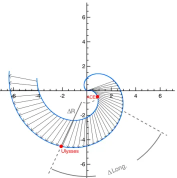
1334 H. A. Elliott et al.: Latitudinal extent -6 -4 -2 2 4 6 -6 -4 -2 2 4 6 ACE Ulysses DR DLong .
Fig. 2. Diagram of LARP method. Blue lines are magnetic field
lines, red dots are spacecraft, and black arrows are velocity vectors. The Sun is at the center and the units of distance are AU.
data (bottom curve). Each of the successive curves is off-set by 40 km s−1in this stacked format. The compressions on the leading edges of high-speed streams become steep-er with distance as faststeep-er plasma ovsteep-ertakes slowsteep-er plasma ahead. Such compressions on the leading edges of corotating interaction regions typically steepen into shocks between 1.5 and 2.5 AU, and can easily be tracked out to distances greater than 5 AU. Through this process, high-speed structures are worn down as momentum and energy are transferred to lower speed plasma. For example, from 1998.24 to 1998.34 and from 1998.4 to 1998.47 the model predicts that the high-speed features are worn down, consistent with Ulysses mea-surements of a more uniform low speed solar wind speed. Between 1998.34 and 1998.4, Ulysses measurements show enhanced speeds, but the peak in the mapped data occurs at a later time. For this large feature between 1998.34–1998.4, ACE and Ulysses electron measurements both show the pres-ence of counterstreaming electrons, indicating that this struc-ture is an ICME. Gosling (1996) reviewed signastruc-tures of I-CMEs in the heliosphere and found that the presence of coun-terstreaming electrons is perhaps the most reliable signature of an ICME.
The RP method does not take into account the longitudi-nal separation of the two spacecraft, which varies between 0◦ and 360◦each year, as the Earth and L1 revolve around the Sun. To compensate for this effect (at least for co-rotating structures), one set of observations has been “de-rotated” with respect to the other. We will refer to the combination of longitude adjustment and radial propagation as LARP. The propagation time for the LARP method can be thought of as the time required for a spiral at ACE to propagate to Ulysses,
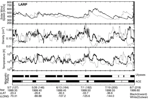
0 5 10 D e n si ty [ c m -3] 1 ACE Model Ulysses Ulysses 2 3 4 5 6 R [AU] 0 5.0x10 4 1.0x10 5 1.5x10 5 Te m p e ra tu re [ K ] ACE Model
Fig. 3. Density and temperature data divided into radial bins and
averaged. Simulation results are shown in grey, ACE and Ulysses data are shown in black. Description of the data set and binning is provided in the text.
as shown schematically in Fig. 2. To examine Ulysses obser-vations at higher latitudes, the LARP method may need to be refined to include the latitude dependence of the spiral wind-ing. The second panel in Fig. 1 overlays the speed profiles after shifting the radially propagated ACE data in time, in or-der to match the ACE source longitudes to the Ulysses ones. Practically, this was accomplished by subtracting the inertial heliospheric longitudes for the two spacecraft and convert-ing this difference into an effective time shift usconvert-ing the solar rotation rate. In order to minimize the effects of temporal evolution of the solar source, the data are rotated the shortest way around (forward or backward in time) so that compar-isons are always made between data separated by less than two weeks. Using the LARP method causes the large fea-ture in the Ulysses data at 1998.34 to align with the double peaked feature in the mapped data.
It appears that the series of peaks observed at ACE either do not merge properly in the model, or parts of an ICME could evolve differently as some ICME model results show (Riley et al., 1997). The LARP method works particularly well for the ICME at 1998.34. In total, we have examined 15 counterstreaming intervals from 1 February 1998 to 31 October 1998, and find that the LARP method improves the sector alignment for 10 of those intervals. There were not enough CME observations to draw definitive conclusions. If an ICME stays magnetically connected to the Sun for a long time, then it becomes aligned along a spiral, as depicted by McComas et al. (1992), such that the westward flank be-comes elongated more than the eastward flank. Also, the spiral angle of such an ICME, as with any magnetically con-nected solar wind flow, depends on the speed of the ICME.
200 300 400 500 600 700 800 S o la r W in d S p e e d [ k m /s ] LARP 0.01 0.10 1.00 D e n si ty [ c m -3] 103 104 105 Te m p e ra tu re [ K ] 1999.35 1999.40 1999.45 1999.50 1999.55 M a g n e ti c P o la ri ty Ulysses ACE Black(Inward) White(Outward) -23.4 -70.31 -26.8 -88.88 -30.3 -107.2 -33.7 -125.6 -36.6 -144.0 DLONG DLAT Year 1999.60 5/7 (127) 5/26 (146) 6/13 (164) 7/1 (182) 7/19 (200) 8/7 (219)
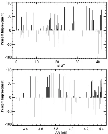
Fig. 4. Similar format as Fig. 1, but
is at a time where ACE and Ulysses have a larger separation in latitude. The top panel shows the solar wind speed ACE data propagated using the LARP method (thin black line) and the Ulysses data (thick black line). Density is shown in the second panel, tempera-ture in the third and sector in the fourth panel.
The bottom three panels of Fig. 1 compare Ulysses density (third panel), temperature (fourth panel), and magnetic po-larity (bottom panel) measurements to the LARP ACE data. The LARP ACE speeds, average density, and temperature agree fairly well with the Ulysses data; however, the high frequency fluctuations in density and temperature do not. We would not expect high frequency fluctuations to agree well because while the two spacecraft observe the same large-scale solar wind structures, they never observe precisely the same parcels of plasma. ACE and Ulysses show very similar sector structure throughout this entire interval. From 1998.31 to 1998.42 the mean mapped density and variations in den-sity agree well with the data. The mapped mean temperature and temperature profile agrees well with the measured tem-perature over a longer time period from 1998.31 to 1998.5, although from 1998.42 to 1998.5 the difference between the model and data average temperature is greater than earlier. It appears that the mapped density and temperatures agree less well than the velocity and sector mainly because the temper-ature and density are such highly variable parameters.
In order to compare the average variations in the mapped density and temperature with the Ulysses observations, we calculated radial profiles. In Fig. 3 the model results from 5 February 1998 through 31 December 1999 are binned in ra-dial distance and averaged over time. The ACE and Ulysses measurements are analyzed similarly, except Ulysses data are taken from 31 December 1997 to 3 March 2001, when Ulysses was moving over radial distances ranging from 1.6 to 5.4 AU. The radial variation of density and temperature observed in the Ulysses data are consistent with the density being proportional to R−2 and temperature proportional to R−1, as shown in a statistical study of Ulysses’ entire first orbit observations (McComas et al., 2000) and calculated in this study by the Zeus model. In the model the R−2 depen-dence is due to spherical expansion, and the temperature
de-pendence is then R−1for a polytropic index of 3/2.
As the latitude separation between the spacecraft becomes larger, ACE and Ulysses do not observe the same features as frequently. The sector structure at ACE and Ulysses are at times similar, however, the plasma parameters do not agree over such large time spans as when the latitude separation was smaller. For example, Fig. 4 shows the interval from 1999.35 to 1999.65, as the latitude separation between the two spacecraft grew from 20◦ to 38◦. The model speed agrees well at the beginning (1999.44–1999.51) when the speed is steady, but the general shape and extent of the first peak (1999.51) does not match well. This may indicate that our mapping has correctly aligned the structures in longi-tude, and the differences reflect the spatial differences of the structure, that is, ACE and Ulysses are probing different parts of a given CIR. Different parts of a CIR or ICME probably have different compression strengths and thicknesses. To-wards the end of this plot the model predicts a peak in ve-locity at 1999.58 that is not observed at Ulysses. It appears that when ACE and Ulysses have large latitude separations the two spacecraft do not encounter the same features as fre-quently as they do at smaller latitude separations.
Inspection of the coronal hole maps shown in Fig. 5, and the electron distributions leads us to believe that we may not be observing the same structures in 1999 when the space-craft become separated by more than 27◦ in latitude. The coronal hole maps in Fig. 5 are derived from He I λ1083 nm Kitt Peak heliospectrograms. Harvey (1996) and Harvey and Recely (2002) use four criteria to determine the boundaries. Those criteria are the coronal holes (1) appear bright in the He I λ1083 nm spectroheliograms, (2) contain between 75% and 100% of one magnetic polarity, (3) are at least 2 super-granules in size, and (4) have low network contrast. Coronal hole boundaries expand in latitude and longitude with alti-tude in the corona, but we still find these maps to provide
1336 H. A. Elliott et al.: Latitudinal extent Carrington Rotation 1951 06/24/1999-07/21/1999 Carrington Rotation 1953 08/18/1999-09/14/1999 Carrington Rotation 1954 09/14/1999-10/11/1999 Carrington Rotation 1952 07/21/1999-08/18/1999
Fig. 5. He I λ1083 nm coronal hole maps from Kitt Peak. Light
grey is outward polarity and dark grey is inward polarity.
valuable qualitative information about the relative size and distribution of coronal holes at high and low latitudes. At first glance the agreement in Fig. 4 looks fairly good, but the coronal hole maps like those in Fig. 5 show that the latitude extent of the coronal holes is less than the latitude separa-tion between the satellites. In mid 1999 ACE and Ulysses were about 28◦apart in latitude, the coronal hole map during this time (Rotation 1951) shows that there are a few small holes. By the end of September (Rotation 1954), many small holes have developed at low latitudes. Furthermore, dur-ing this time period coronal holes of like polarity occur near each other, which makes it more difficult to determine if both spacecraft are observing plasma from the same coronal hole.
Examination of ACE and Ulysses superthermal electron data show that counterstreaming occurred at different times at the two spacecraft during the interval shown in Fig. 4, indicating that the structures observed at ACE do not generally map to those observed at Ulysses.
Using the plasma and magnetometer data we find that once the spacecraft are separated by more than 28◦, the same structures are not observed at both spacecraft, since after this point the sector structure at both spacecraft starts to become different, but more importantly, the ion and electron mea-surements indicate different structures. Thus, during the ris-ing phase of 1999 the streams were much smaller than the polar coronal holes observed with Ulysses during solar min-imum conditions. However, smaller structures in the helio-sphere are consistent with the solar coronal hole maps that show the presence of small coronal holes.
When we examine the data for spacecraft latitude separa-tions between 0◦ and 42◦, there are many instances where both spacecraft appear to observe very similar sectors. We have calculated the difference between the fractions of the inward sector in the model and the measured intervals. Fig-ure 6 shows an example where we have defined boundaries of given regions in the ACE data and then tracked those bound-aries by advancing them at each time step in the simulation, using the velocity and acceleration at that grid point. The data are categorized into four groups: high-speed streams (h), counterstreaming electrons (c), other (o), (mostly slow solar wind), and data gaps (g). Data gaps were interpolated to allow for long simulation runs. The data gap intervals are not included in our analysis. In Fig. 6 a given region can easily be tracked using the alternating grey and white bands of adjacent regions. For the ACE and Ulysses data curves in Fig. 6, red indicates the outward sector, and black indicates the inward sector. We compared the amount of the inward sector for the Ulysses curve to the amount of the inward sec-tor observed back at ACE for the modeled interval using both the radial propagation and the LARP methods.
In Fig. 7 the percent differences for these two methods of propagation are shown. Points along the 45◦ line have the same level of agreement for both methods. The source lon-gitude adjustment improves the level of agreement (smaller percent differences) over the radial method. When the source longitude method does not improve the level of agreement, the data points still lie near the 45◦line. In Fig. 7, two-thirds of the points lie above the 45◦line, which means many inter-vals are improved with the source longitude adjustment. In Fig. 8 we examine the difference between the data and model fraction of the inward sector for a given interval, as a func-tion of the separafunc-tion between the spacecraft. Figure 8 shows that the LARP method often improves the sector agreement significantly compared to the RP method. At latitude separa-tions greater than 27◦the percentage improvement tends to be larger (black bars). The Ulysses orbit is such that larger latitude separations between the spacecraft occur at smaller radial separations; hence, the percent improvement is larger at distances less than 4 AU.
2500 2000 1500 1000 500 1998.25 1998.30 1998.35 1998.40 1998.45 1998.50 Year 1998.25 1998.30 1998.35 1998.40 1998.50 Year 90 30 -30 -90 0 U ly -L a t ( ) S o la r W in d S p e e d ( k m /s ) Ulysses (R)=5.40 AU DLon DLon Uly-Lat 1998.45 LARP o c h c c c o c c gc h c c c 1.00 AU 1.70 AU 2.40 AU 3.10 AU 3.79 AU 4.49 AU Closest 5.39 AU 180 90 -90 0 -180 0 D L o n ( ) 0 D L o n ( ) ACE Inward Outward Ulysses Model
Fig. 6. Same data as in Fig. 1, but now the common source longitude ad-justment has been included. The data is divided into regions with vertical bars. These points are then kept track of with in the simulation as they propagate out-ward. Alternating grey and white shows
how regions propagate. The arrow
shows how one of the region propagates from 1 AU out 5.4 AU. Above each re-gion is a label indicating the classifica-tion. O for other, c for ICME, h for high-speed stream, and g for data gap. For the ACE and Ulysses curves, red is outward sector, and black is inward.
5 Conclusions
We utilized a directly driven hydrodynamic model to com-pare structures observed at ACE in the ecliptic plane near 1 AU with those observed at various heliolatitudes and greater heliocentric distances by Ulysses. The radial varia-tion of the average density and temperature observed in the Ulysses data are consistent with the density being propor-tional to R−2 and temperature proportional to R−1. How-ever, many specific features in the speed, density and tem-perature are worn down by stream interactions by the time they reach Ulysses.
At smaller latitude separations, particularly less than
∼15◦, ACE and Ulysses frequently observe parts of the same stream structures. At greater latitude separations this asso-ciation tends to break down with little correlation left by the time Ulysses reaches ∼30◦ latitude. The association breaks down well before Ulysses reaches high enough south-ern latitudes, such that only one magnetic polarity is ob-served. Smith et al. (2001) examined Ulysses observations from years 1999 and 2000, and they found that two mag-netic sectors were present up to a latitude of −78◦. The LARP method, which corrects for longitude separations be-tween the two spacecraft, generally improves sector align-ment, even for greater latitude separations. This reflects the large-scale nature of the sector structure, consistent with the fact that the sector structure generally corotates. The He I λ1083 coronal hole maps show that the number of low-latitude coronal holes increases in 1999 and that ACE and Ulysses frequently pass close to, and may be sampling plasma from, different coronal holes once the latitude sepa-ration becomes significant. We found many instances where there were small coronal holes of the same magnetic polarity that were near each other and had latitude separations smaller
0 20 40 60 80 100 Sector % Difference LARP 0 20 40 60 80 100 S e c to r % D iff e re n c e R a d ia l P ro p a g a ti o n
Fig. 7. Percent difference between the amount of inward sector for
the model and data intervals. The x-axis uses intervals determined using the radial propagation and the source longitude adjustment. The y-axis is only using the radial propagation.
than the latitude separation of the spacecraft. In such cases the sector structure may be similar, but comparisons between the predicted plasma properties and the Ulysses plasma mea-surements often break down. Also at these larger latitude separations, instances when the predicted speeds, densities, and temperatures matched frequently appeared to reflect the fact that coronal hole flows tend to have similar plasma
prop-1338 H. A. Elliott et al.: Latitudinal extent 3.4 3.6 3.8 4.0 4.2 4.4 DR [AU] -100 -50 0 50 100 P er ce nt I m pr ov em en t 0 10 20 30 40 DLAT -100 -50 0 50 100 P er ce nt I m pr ov em en t
Fig. 8. Amount of improvement in sector agreement. Cases where
the source longitude adjustment agreed better with the model are shown in black and cases where the radial propagation along agreed better are shown in grey. The length of the lines represents the dif-ferences in the level of agreement for the two methods.
erties. This similarity makes it difficult to determine when ACE and Ulysses were measuring plasma from the same coronal holes. A further complication is that while coronal hole properties are distinct from those of the slow solar wind, flows from Coronal Hole Boundary Layers (CHBLs) provide solar wind plasma with intermediate speeds and heavy ion freezing-in temperatures that span the range between these two types of flows (McComas et al., 2002b); the measured properties of CHBL flows are highly dependent on exactly where a spacecraft passes through them.
In this study we have utilized a directly driven hydrody-namic model to compare observations between widely sepa-rated spacecraft. Using ACE and Ulysses measurements we found that during the rising phase of solar cycle 23 stream structures in the heliosphere measured 20–30◦ in heliolati-tude. Our comparison shows that stream structures derived from smaller coronal holes during the rising phase of solar cycle 23 persist over 20–30◦in heliolatitude, consistent with solar observations, indicating the presence of small coronal holes.
Acknowledgements. We thank N. Ness and C. Smith for use of
the ACE magnetometer data, A. Balogh for use of the Ulysses magnetometer data, and K. Harvey and J. Harvey for making the NSO/Kitt Peak coronal hole maps readily available. The NSO/Kitt
Peak data used here were produced cooperatively by NSF/NOAO, NASA/GSFC, and NOAA/SEL. We thank the reviewers. This work was supported by NASA’s ACE and Ulysses programs as a part of the SWEPAM and SWOOPS data analysis efforts and by the NASA SEC-GI program.
Topical Editor R. Forsyth thanks A. Szabo and another referee for their help in evaluating this paper.
References
Balogh, A., Beek, T. J., Forsyth, R. J., Hedgecock, P. C., Mar-quedant, R. J., Smith, E. J., Southwood, D. J., and Tsurutani, B. T.: The magnetic field investigation on the Ulysses mission: Instrumentation and preliminary scientific results, Astron. and Astrophys. Suppl. Ser., 92, 221–236, 1992.
Bame, S. J., McComas, D. J., Barraclough, B. L., Phillips, J. L., Sofaly, K. J., Chavez, J. C., Goldstein, B. E., and Sakurai, R. K.: The Ulysses solar wind plasma experiment, Astron. and Astro-phys. Suppl. Ser., 92, 237, 1992.
Belcher, J. W. and Davis, Jr., L.: Large-amplitude Alfv´en waves in the interplanetary medium, 2, J. Geophys. Res, 76, 3534–3563, 1971.
De Keyser, J., Roth, M., Forsyth, R., and Reisenfeld, D.: Ulysses observations of sector boundaries at aphelion, J. Geophys. Res., 105, 15 689–15 698, 2000.
Feldman, W. C., Barraclough, B. L., Phillips, J. L., and Wang, Y.-M.: Constraints on high speed solar wind structure near its coro-nal base: A Ulysses perspective, Astron. Astrophys., 316, 355– 367, 1996.
Forsyth, R. J., Balogh, A., Smith, E. J., Erd¨os, G., and McComas, D. J.: The underlying Parker spiral structure in the Ulysses mag-netic field observations 1990–1994, J. Geophys. Res., 101, 395– 403, 1996.
Geiss, J. G., Gloeckler, von Steiger, R., Balsiger, H., Fisk, L. A., Galvin, A. B., Ipavich, F. M., Livi, S., McKenzie, J. F., Ogilvie, K. W., and Wilken, B.: The southern high-speed stream: Results from the SWICS instrument on Ulysses, Science, 268, 1033– 1036, 1995.
Gosling, J. T.: Corotating and transient solar wind flows in three dimensions, Annu. Rev. Astron. Astrophys., 34, 35–73, 1996. Gosling, J. T.: Coronal mass ejections: an overview, in:
Coro-nal Mass Ejections, (Eds) Crooker et al., vol. 99 of Geophysical Monograph, pp. 9–15, AGU, Washington D. C., 1997.
Gosling, J. T., McComas, D. J., Phillips, J. L., Pizzo, V. J., Gold-stein, B. E., Forsyth, R. J., and Lepping, R. P.: A CME-driven so-lar wind disturbance observed at both low and high heliographic latitudes, Geophys. Res. Lett., 22, 1753–1756, 1995.
Gosling, J. T., Riley, P., McComas, D. J., and Pizzo, V. J.: Over-expanding coronal mass ejections at high heliographic latitudes: Observations and simulations, J. Geophys. Res., 103, 1941– 1954, 1998.
Harvey, K. L.: Coronal structures deduced from photospheric mag-netic field and He i λ10830 observations, in: Solar Wind Eight, (Eds) Winterhalter et al., pp. 9–13, Am. Inst. Of Phys., Wood-bury NY, 1996.
Harvey, K. L. and Recely, F.: Polar coronal holes during cycles 22 and 23, Solar Phys., submitted, 2002.
Hundhausen, A. J.: An interplanetary view of coronal holes, in: Coronal Holes and High Speed Streams, (Ed) J. B. Zieker, pp. 223–329, Colo. Assoc. Univ. Press., 1977.
Hundhausen, A. J., Hansen, R. T., and Hansen, S. F.: Coronal evo-lution during the sunspot cycle: Coronal holes observed with the mauna loa k-coronameters, J. Geophys. Res., 88, 2079–2094, 1981.
McComas, D. J., Gosling, J. T., and Phillips, J. L.: Interplanetary magnetic flux: Measurement and balance, J. Geophys. Res., 97, 171–177, 1992.
McComas, D. J., Bame, S. J., Barker, P., Feldman, W. C., Phillips, J. L., Riley, P., and Griffee, J. W.: Solar wind electron proton alpha monitor (SWEPAM) for the Advanced Composition Ex-polorer, Space Sci. Rev., 86, 563–612, 1998.
McComas, D. J., Barraclough, B., Funsten, H., Gosling, J. T., Santiago-Mu˜noz, E., Skoug, R. M., Goldstein, B., Neugebauer, M., Riley, P., and Balog, A.: Solar wind observations over Ulysses’ first full polar orbit, J. Geophys. Res., 105, 10 419– 10 433, 2000.
McComas, D. J., Elliott, H. A., Gosling, J. T., Reisenfeld, D., Sk-oug, R. M., Goldstein, B., Neugebauer, M., and Balogh, A.: Ulysses’ second fast-latitude scan: Complexity near solar max-imum and the reformation of polar coronal holes, J. Geophys. Res., 101, 10.1029/2001GL01 416, 2002a.
McComas, D. J., Elliott, H. A., and von Steiger, R.: Solar wind from high latitude coronal holes at solar maximum, Geophys. Res. Lett., 29, 10.1029/2001GL013 940, 2002b.
Mitchell, D. G., Roelof, E. C., and Wolfe, J. H.: Latitude depen-dence of solar wind velocity observed at 1au, J.Geophys. Res., 86, 165–179, 1981.
Neugebauer, M. and Goldstein, R.: Particle and field signatures of coronal mass ejections in the solar wind, in: Coronal Mass Ejec-tion, (Ed) Crooker et al., vol. 99 of Geophysical Monograph, pp. 245–251, AGU, Washington D. C., 1997.
Neugebauer, M., Forsyth, R. J., Galvin, A. B., Harvey, K. L., Hoek-sema, J. T., Lazarus, A. J., Lepping, R. P., Linker, J. A., Mikic, Z., Steinberg, J. T., von Steiger, R., Wang, Y., and Wimmer-Schweingruber, R. F.: Spatial structure of the solar wind and comparisons with the solar data and models, J. Geophys. Res., 103, 14 587–14 599, 1998.
Neugebauer, M., Liewer, P. C., Smith, E. J., Skoug, R. M., and Zur-buchen, T. H.: Sources of the solar wind at solar activity maxi-mum, J. Geophys. Res., 107, 10.1029/2001JA000 306, 2002. Richardson, J. D., Paularena, K. I., Wang, C., and Burlaga, L. F.:
The life of a CME and the development of a MIR: From the sun to 58 au, J. Geophys. Res., 107, 10.1029/2001JA000 175, 2002. Riley, P. and Gosling, J. T.: Do coronal mass ejections implode in
the solar wind, Geophys. Res. Lett., 25, 1529–1532, 1998. Riley, P., Gosling, J. T., and Pizzo, V. J.: A two-dimensional
simu-lation of the radial and latitudinal evolution of a solar wind dis-turbance driven by fast, high-pressure coronal mass ejection, J. Geophys. Res., 102, 14 677–14 685, 1997.
Riley, P., Gosling, J. T., and Pizzo, V. J.: Investigation of the poly-tropic relationship between density and temperature within inter-planetary coronal mass ejections using numerical simulations, J. Geophys. Res., 106, 8291–8300, 2001.
Riley, P., Linker, J. A., and Mikic, Z.: Modeling the heliospheric current sheet: Solar-cycle variations, J. Geophys. Res., 107, 10.1029/2001JA000 299, 2002.
Schwenn, R., M¨uhlh¨auser, K.-H., and Rosenbauer, H.: Two states of the solar wind at the time of the solar activity minimum, I. Boundary layers between fast and slow streams, in: So-lar Wind Four, pp. 118–125, Max-Planck-Inst. f¨ur Aeronomie, Katlenburg-Lindau MPAE–W–100–81–31, 1981.
Smith, C. W., Acu˜na, M. H., Burlaga, L., L’Heurex, J., Ness, N. F., and Scheifele, J.: The ACE magnetic fields experiment, Space Science Reviews, 86, 613–632, 1998.
Smith, E. J., Balogh, A., Forsyth, R. J., and McComas, D. J.: Ulysses in the south polar cap at solar maximum: Heliospheric magnetic field, Geophys. Res. Lett., 28, 4159–4162, 2001. Stone, J. M. and Norman, M. L.: ZEUS-2-D: A radiation
magneto-hydrodyanmics code for astrophysical flows in two dimensions I The hydrodynamic algorithms, and tests, Astrophys. J., 80, 753, 1992.
Wang, C., Richardson, J. D., and Gosling, J. T.: A numerical study of the evolution of the solar wind form Ulysses to Voyager 2, J. Geophys. Res., 105, 2337–2344, 2000a.
Wang, C., Richardson, J. D., and Gosling, J. T.: Slowdown of the solar wind in the outer heliosphere and the interstellar neutral hydrogen density, Geophys. Res. Lett., 27, 2429–2431, 2000b. Wang, Y. M., Hawley, S. H., and Sheeley Jr., N. R. S.: The magnetic
nature of coronal holes, Science, 271, 464–469, 1996.
Webb, D. F. and Howard, R. A.: The solar cycle variation of coronal mass ejections and the solar wind mass flux, J. Geophys. Res., 99, 4201–4220, 1994.