Domain Partitioning to Bound Moments of
Differential Equations Using Semidefinite
Optimization
by
Sandeep Sethuraman
Submitted to the School of Engineering
in partial fulfillment of the requirements for the degree of
Master of Science in Computation for Design and Optimization
at the
MASSACHUSETTS INSTITUTE OF TECHNOLOGY
September 2006
©
Massachusetts Institute of Technology 2006. All rights reserved.
Author ...
School of Engineering
Certified by.
/
August 10, 2006
Pablo A. Parrilo
Associate Professor
Thesis Supervisor
Accepted by.
Jaime Peraire
OF TECHNOLOGYSEP
13 2006
LIBRARIES
Professor of Aeronautics and Astronautics
r c or, ompu a on or es gn an p mza on rogram ARCHIVES 2
I IA
.
..
.
.
.
.
..
.
.
..
.... .
Codiet C tti f D i d O ti PDomain Partitioning to Bound Moments of Differential
Equations Using Semidefinite Optimization
by
Sandeep Sethuraman
Submitted to the School of Engineering on August 10, 2006, in partial fulfillment of the
requirements for the degree of
Master of Science in Computation for Design and Optimization
Abstract
In this thesis, we present a modification of an existing methodology to obtain a hierar-chy of lower and upper bounds on moments of solutions of linear differential equations. The motivation for change is to obtain tighter bounds by solving smaller semidefi-nite problems. The modification we propose involves partitioning the domain and normalizing each partition to ensure numerical stability. Using the adjoint operator, linear constraints involving the boundary conditions and moments of the solution are developed for each partition. Semidefinite constraints are imposed on the moments, and an optimization problem is solved to obtain the bounds. We have demonstrated the algorithm by calculating bounds on moments of various one-dimensional case differential equations including the Bessel ODE, and Legendre polynomials. In the two-dimensional case we have demonstrated the algorithm by calculating bounds on various PDEs including the Helmholtz equation, and heat equation. In both cases, the results were encouraging with tighter bounds on moments being obtained by solving smaller problems with domain partitioning.
Thesis Supervisor: Pablo A. Parrilo Title: Associate Professor
Acknowledgments
I would like to express my thanks to a number of individuals for their contributions to this thesis in particular, and my time at MIT as a student.
First, I would like to thank my adviser, Pablo Parrilo, for the many hours of guidance and encouragement. It has been an amazing experience working under his supervision, and I will be forever thankful for this opportunity.
My gratitude extends to Constantine Caramanis, who helped tremendously in understanding his work, and provided thoughtful insights during the course of the project. Professor Bertismas's encouragement during the course of the project was very useful. I want to thank J. Ldfberg for writing and making freely available his excellent software YALMIP [11], and for his guidance and advice during code development. I am grateful to Singapore-MIT Alliance for their financial support.
I would also like to thank my friends Anu, Harish, Ram and Ruchi, with whom I have had some wonderful experiences, and whose friendship I will value for life; Sukant and Ashish, friends who with their good humor made my time at MIT totally unique by making sure I was not stuck in my lab all day and all night. I am grateful to Mabel for helping me with my thesis tremendously, and for proofreading it more times than I myself might have done. Hu Sha, Sun Jiali, Homan, Shawn and Georgios with their friendship and conversation made the days and many nights in LIDS much more enjoyable.
I owe my deepest thanks to my parents Beena and Sethuraman, and my ever loyal sister Lakshmi, for their unconditional support, and their belief in me all these years. They have done the best job of being family when family was needed. I owe them more than I would be able to express.
Contents
1 Introduction
1.1 Standard solution techniques for PDEs . . . . 1.1.1 Finite difference method . . . ... 1.1.2 Spectral methods ... ...
1.1.3 Finite element method . ...
1.2 Moment calculation using semidefinite optimization 2 Description of the method
2.1 Basic approach - theory . . . . . 2.2 Adjoint operator . . . ... 2.3 Definitions . ...
2.4 Moments and moment matrices . 2.5 Semidefinite constraints . . . . . 2.6 Motivation for modification . . . 2.6.1 Proposed modification . .
3 One dimensional case - ordinary differential equations(ODEs) 3.1 Partitioning and change of domain / domain mapping ...
3.1.1 Scaling of constant coefficients . ... 3.1.2 Scaling of non-constant coefficients . ... 3.1.3 New boundary variables . ... 3.2 3.3 Adjoint operator ... Coupling conditions ... 15 . 16 . 17 . 18 . 20 . 21 23 .. . . . . 23 . . . . . . . 24 . . . . . . . 26 .. . . . . 26 . . . . . . . 28 .. . . . . 31 .. . . . . 32
3.4 3.5 3.6 3.7 3.8 3.9 3.10 3.11
Right hand side . ... Substituting . . . ... SDP constraints . ... Solving the system . ... Recovering original moments ... Brief summary ... Higher order ODEs ...
Implementation for testing purposes . 4 Numerical validation
4.1 Examples - plots and error plots . . . . 4.1.1 ODEs with closed form solution . . 4.1.2 ODEs with no closed form solution 4.2 Discussion . . ...
4.2.1 Accuracy of solution . . . . 4.2.2 Running time . ...
4.2.3 Inferring the solution . . . .
4.2.4 Summary ... ...
5 Second order two-dimensional partial differential equations 5.1 Partitioning and domain transformation . . . ..
5.1.1 Constant coefficients .... .... . . . . .. . . . .. 5.1.2 Non-constant coefficients . .. . . .. ... 5.2 Adjoint Operator ... . . . . . . . ... ...
5.2.1 Moment variables . ... . ...
5.3 Calculating boundary and derivative boundary moments in the new domain and coupling conditions . . . . . . . . .. 5.3.1 Coupling conditions ... . . . . . . . . .... 5.4 Right hand side . ....
5.5 Substituting 0 ... 5.6 SDP constraints . ... . . . . . . . . . .. 42 .. . . . . 43 51 ... . . . . . . 51 . . . . . . . . 53 . . . . . . . . . . 53 . . . . . . . 53 .. . . . . 53 . . . . . 62 .. . . . . 63 .. . . . . 65 67 68 70 70 71 73 74 75 76 76 77
5.7 5.8
5.6.1 Moment matrices . 5.6.2 Boundary moments Recovering the moments . Implementation ... 6 Numerical validation
6.1 Two-dimensional PDEs ... 6.1.1 Poisson's equation ...
6.1.2 Helmholtz equation ... ...
6.1.3 Non-constant coefficient example . . . .. 6.1.4 Heat equation . .... ...
6.2 Discussion . . . . ...
6.2.1 Accuracy for lower degree test functions . . . . 6.2.2 Numerical problems . ...
6.2.3 Reduction of feasible region . . . .... 6.2.4 Relaxation of constraints . . . ...
6.3 Summary ... ...
7 Conclusions and future directions
A Expansion of terms in the two-dimensional equations
79 .. . . . . 80 .. . . . 80 .. . . . . 81 .. . . . 82 .. . . . . 82 .. . . . . 83 . . . . . 83 .. . . . . 84 .. . . . . 85 .. . . . . 86 .. . . . . 86
List of Figures
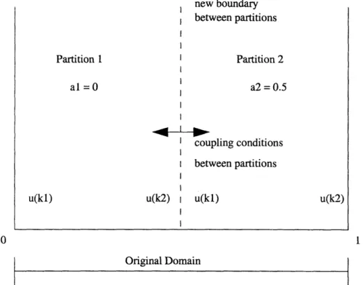
3-1 Partitioning the domain into D partitions. Each partition is mapped on to a new domain [-1, 1]. The start and end of each partition are indicated by ai and bi respectively. . ... 35 3-2 Partitioning of the domain into two regions. The dotted line indicates
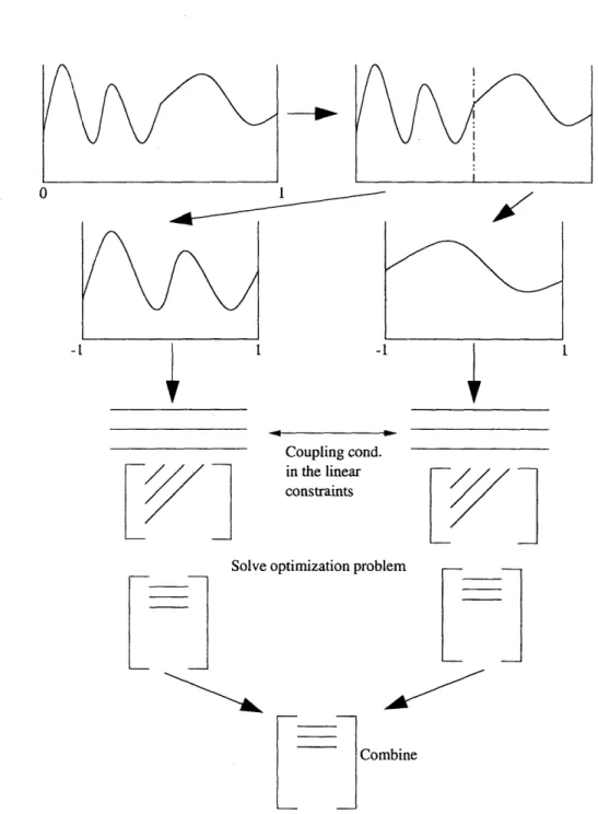
the new boundary with the coupling conditions .... ... 37 3-3 Brief Summary of Algorithm - The original domain is partitioned and
each partition is transformed to a normalized scale. Using the adjoint operator linear constraints are generated. Coupling conditions between partitions, and SDP constraints are also written and the optimization problem is solved. Finally, the original moments of the system are recovered by combining the moments corresponding to each partition. 47 4-1 Plot and error in the solution to ODE u" + 12u' + 50u = 4, u'(0) =
5,u'(1) =0 .... ...
...
...
...
54
4-2 Plot, and error in the solution to ODE u" + 3u' - 4u = 0, u'(0) =-1,u'(1)=0 . ... ... 55
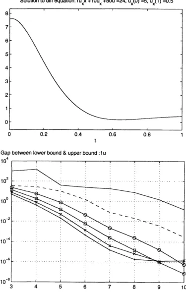
4-3 Plot and error in the solution to ODE u" + 10u' + 50u = 24, u'(O) =
5,u'(1)=0.5 ... ... 56
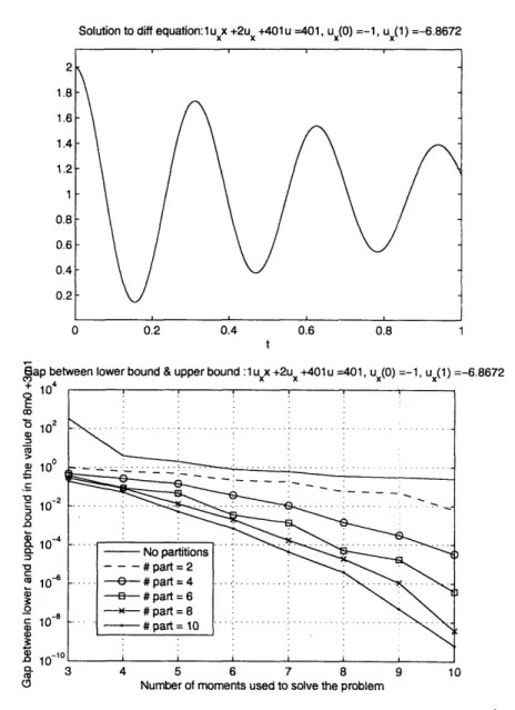
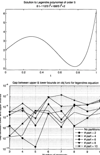
4-4 Plot and error in the solution to ODE u" + 2u' + 401u = 401, u'(1) = - 1,u'(1) = -6.872 ... ... 57 4-5 Plot and error in the solution to a 5th order Legendre Polynomials.
This example demonstrates that ODEs with polynomial solution do not benefit by partitioning the domain. . ... 58
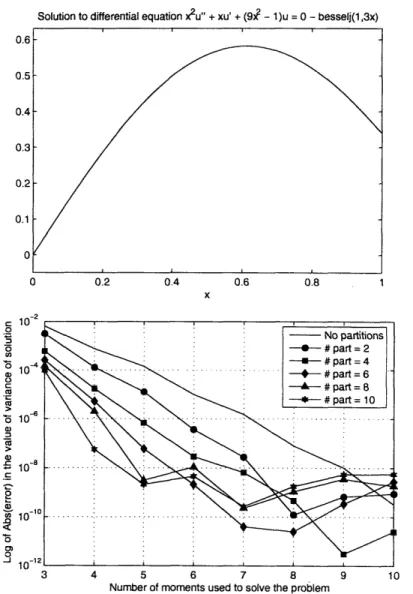
4-6 Plot and error in the solution to ODE x2u"+u'+(9'2-1)u = 0, u'(0) =
1.5, u'(1) = Jo(3) - J2(3). Solution is the Bessel function
Ji(3x)
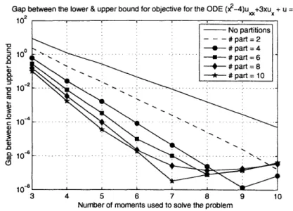
. . . 59 4-7 Gap between upper and lower bound for 8mo + 3ml for the ODE( 2 - 4)u" + 3u' + u = 0 ... .... ... 60 4-8 Time taken to compute the lower and upper bounds on the objective
for the ODE : u" + 2u' + 401u = 401 ... 62 4-9 Graph showing the solution, and the bounds on mo for the ODE ux +
3ux - 4u = 0, ux(0) = -1, u.(1) = 0 with no partitions. The average
value does not indicate very well what is happening in the domain . . 63 4-10 Graph showing the solution, and the bounds on mo for the ODE uzx +
3ux - 4u = 0, u.(0) = -1, u;(1) = 0 with 4 partitions. The average
values of the four partitions indicate better what is happening in the
domain ... ... 64
5-1 Sketch of the partition of the two-dimensional region. The arrows on the dotted line indicate the coupling conditions between partitions. . 69 6-1 Gap between lower bound and upper bound for ml,0 of the differential
equation Au = 4 sinh(x) cosh(x) + 4 cosh(y) sinh(y) . ... 80 6-2 Gap between lower bound and upper bound for mo0,0 of the differential
equation Au
+
u = 3ex+y . . . .. ... . . . . . . .... . . . ... 816-3 Gap between lower and upper bound in value of ml,0 of the equation
Uy =: X4Uxx+..U ... . . ... .83
6-4 Gal) between lower and upper bound for value of ml,0 for the heat
equation u2z - uy + u = 0. For the bigger partitions, SeDuMi runs
into numerical problems, and stops solving the optimization with a bigger gap between the dual and primal problems. . ... . .84
List of Tables
4.1 Lower and Upper bounds on the value of 8mo + 3ml of the solution of ODE 'u" + 2u' + 401u = 401, u(1) = -1, u'(1) = -6.872' using
no-partitions ... ... ... 52
4.2 Lower and Upper bounds on the value of 8mo + 3ml of the solution of ODE 'u" + 2u' + 401u = 401, u'(1) = -1, u'(1) = -6.872' using 4
Chapter 1
Introduction
Quantities that depend on space and/or time variables are governed by differential equations based on underlying physical principles. Partial Differential Equations (PDEs) not only accurately express these principles, but also help to predict the be-havior of a system from an initial state of the system and given external influences. They are used to formulate and solve problems that involve unknown functions of several variables, such as the propagation of sound or heat, electrostatics, electrody-namics, fluid flow, elasticity, or more generally any process that is distributed in space, or space and time. Very different physical problems may have identical mathematical
1.1
Standard solution techniques for PDEs
Generally, partial differential equations can be represented as
Lu
where
L
U
=f in Q,
the problem domain in which we are interested in solving, a differential operator,
the unknown field variable in the domain 0,
f is the forcing function.
In order to obtain an unique solution to the unknown field, boundary conditions have to be specified. A detailed description on applying boundary conditions can be found elsewhere. For example, the steady state heat conduction equation is given as,
-V. (KVT)
T
-K (VT.n) = q in Q, = To on aQD, =q
0 on 80N, where,K is the thermal conductivity of the material,
T is the unknown temperature field we wish to compute, q is the heat generated per unit volume,
Q is the domain in which we are interested in solving the problem (QD is the Dirichlet boundary,
8
QN is the Neumann boundary,
To is the temperature field specified on Dirichlet boundarylaQD
qo is the heat flux leaving/entering the
problem domain specified on Neumann boundaryaQN.
The governing differential equations with the boundary conditions specified on the problem domain can be completely solved analytically/approximately depending on the complexity of the problem.
The first approach towards solving these equations involves finding a analytical solution of the equation over the whole domain. There are well established analyti-cal methods for obtaining solutions for a wide variety of partial differential equations. Usually, analytical solutions are available for partial differential equations over regular domains (rectangular, circular) and some other simple cases. However, most engineer-ing problems have complex geometric domains and nonlinear properties. Thereby, it becomes imperative to rely increasingly on numerical techniques to solve PDEs in order to understand and control the systems governed by them.
A few well established techniques for solving PDEs numerically are the Finite Dif-ference method, the Spectral method and the Finite Element method. The following sections will give a brief description on these methods. There is a plethora of literature available on the mathematical aspects of these methods, numerical implementation, practical applications and limitations of these methods [1,3, 4, 6, 7, 9, 10, 12, 13, 17, 20].
1.1.1
Finite difference method
The main idea of the finite difference method is to approximate the differential oper-ator with a difference operoper-ator. The domain is discretized into grid points which can be uniformly spaced (referred to as structured grids) or non uniformly spaced (un-structured grids). The differential operator at each grid point is then expressed using the values at the grid point and its neighbors, this is usually referred to as a stencil. A stencil could be obtained using Taylor series expansion of the derivatives about a
grid point or by other well established techniques [7, 20]. For example, consider the following one dimensional problem,
d2u
d 2 XE[L, R],[
and UIX=XL = 0, u z=,, = 0 imposed as the boundary conditions. The domain is discretized into uniformly placed grid points xi given by
(xR - XL) (i - 1)
Xi = XL + 10 V iE[1..11].
The finite difference approximation at each grid point xi obtained using a central difference scheme would be
Ui+1 - 2Ui + ui-1 ±2A= fif V i[10]ie [2..10]. 2Ax
where ui denotes the value of the unknown field at grid point i, Ax = zi - xi-1 and fi P f an approximation to the actual forcing function. ul and ull (the boundary
points) are equal to zero (due to boundary conditions). The above set of simultaneous equations can be solved to obtain the unknown field at each grid point. It can be seen that the finite difference systems of equations is sparse in nature. This linear system can be solved in a variety of techniques such as Gaussian elimination, QR factorization, Conjugate gradient or even iterative schemes such as Jacobi, or Gauss-Seidel method [14].
1.1.2
Spectral methods
In spectral methods, the solution to the governing partial differential equation Lu = f, is assumed to be approximated by a superposition of smooth global analytic functions [3,4,6,9, 12],
N
U(X) eU2N(X) =E
an
(x),
where UN(X) is the best approximation to u(x) in the space spanned by {0o, ¢i, ..-NY}.
Subsequently, this is substituted into the governing equation and multiplied with a test function v; finally the residual is minimized over the entire domain.
v (Lu - f)dA=O V vEX.
residual
Based on the choice of v (test function) and the interpolation scheme for u (trial function), several numerical schemes can be obtained. Spectral methods use global basis functions in which the ¢,(x) is a polynomial (or trigonometric polynomial) of high degree which is non-zero, except at isolated points, over the entire computational domain. A Galerkin method would be obtained if the same expansion is used for the test function and the trial function [7, 17]
an I(LOm L Enn (x) dAdA=
mfdA
V me 1..N.( n=O
The above can be written in matrix form as
n=1
where Lmn
=-fo mL¢n(x)dA, and fm = fn
m•fdA.The unknown's an are obtained
by solving the above set of linear equations. Typically in a Galerkin method, each of the test/trial functions are chosen so that the boundary conditions are automatically satisfied. Alternatively, the boundary conditions can be imposed as additional con-straints to the linear equation; this class of methods is usually referred to as the Tau methods [12].
Test functions can be chosen as Dirac-delta functions at specific points in the domain. These classes of methods are usually referred as Collocation or
Pseudospec-tral methods and the points chosen are called the collocation points. The boundary conditions can then be applied in the way it is done for Tau methods, as additional
constraints,
j6(x-xm)(Lu -
f)dA
= 0 V m {1..N}.Collocation methods lead to a set of algebraic equations which are given as
N
E3Lmna
=
fmin.
n=1
where Lmn = fo Lq,$(x)dA and f
m= fn Omf dA.
Usually spectral methods deploy polynomials of high order (typically Fourier series or Chebyshev and Legendre polynomials), which gives high accuracy for a given N. Although the generated equations result in full matrices, using fast iterative matrix solvers these techniques can be more efficient than finite element or finite difference methods for many classes of problems [3]. If the geometry of the problem is smooth and regular, these techniques prove to be very useful.
1.1.3
Finite element method
Finite element method in concept is very similar to a Galerkin approach in Spectral methods. The major difference is that this technique uses piecewise low-order polyno-mial functions, instead of the high-order polynopolyno-mial functions [1, 10, 13, 17]. Another difference is that the finite element method relies on the weak form instead of using the strong form of the equation. A weak form is obtained by integrating by parts, the Galerkin weighted residual statement of the governing differential equation. There is extensive literature available on mathematical aspects of finite element analysis and applications that involve solving real-life problems.
There are several commercial software packages available that simulate a system using finite element analysis. The major advantage of finite element analysis is that it can handle complex geometries, non-linearity, interfaces and jumps in the problem domain with little or no extra effort. The disadvantage is low accuracy (for a given
number of degrees of freedom N) because each basis function is a polynomial of low degree [10, 13].
1.2
Moment calculation using semidefinite
opti-mization
Many times instead of an actual solution of a PDE, a particular functional of the solution might be more of interest. For example we might be more concerned with the average temperature along a physical boundary rather than the entire distribution of temperature in a mechanical device. Therefore, under such circumstances solving
the PDE in the entire domain of the solution serves no purpose.
Recently, Bertsimas and Caramanis [2] proposed a technique that can be used to calculate the moments of the solution based on optimization techniques without calculating the actual solution. A plethora of information about a solution can be obtained from the moments of the solution.
The key steps in the proposed scheme in [2] are:
* Write a set of linear equations involving the unknown moments (of the solution), and the boundary conditions. The number of equations generated are equal to the number of moments that we are interested in.
* Construct matrices using the unknown moments in a particular manner. These matrices are required to be positive semidefinite.
* Solve an optimization problem comprising of the linear constraints and the semidefinite constraints.
The accuracy of the moments obtained is enhanced by increasing the number of linear equations. However, this will also increase the size of the semidefinite matrices; hence the problem becomes bigger, which can lead to numerical instability. Thus, we have proposed a modification to the methodology. A detailed description of the existing methodology is presented later.
Structure of the paper
This thesis is structured as follows: In Section 2, we briefly summarize the proposed approach. In Chapter 3, we show the modified algorithm, and derive the formulation for the one-dimensional problem. Chapter 4 shows the numerical validation for the one-dimensional case. In Chapter 5, the two-dimensional formulation is presented, followed by numerical examples in Chapter 6. And lastly, Chapter 7, contains the concluding remarks.
Chapter
Description of the method
As mentioned earlier, this method is based on a modification of the technique proposed by Bertsimas and Caramanis [2]. Hence, a brief summary of the original algorithm is provided below, followed by a summary of the proposed technique.
2.1
Basic approach
-
theory
Given a problem domain Q, and a linear PDE of the form
Lu(x) = f(x),
including the appropriate boundary conditions on functional of the solution,
M0,
we wish to solve for some linearGu(x)dx.
Henceforth, for convenience, we will simply write the equation as
Lu = f.
Since an operation on both sides of the equation should give us identical results, we can multiply by a given class of test functions 7D and integrate both sides of the
equation as
Lu
=f
ý
f
(Lu)= f(f),
VG
D.We can choose a set of functions F = ¢1, k2 ... that is a dense subset of D. Therefore, by linearity of integration we have
Lu= f (Lu) = /(f)4, Vq ED 4= /(Lu) i = (f ) O, V E $F
Although in
p2],
the authors have demonstrated the use of various classes of test func-tions, we shall be primarily concerned with monomials of the form xa = 1x x2•....xd2.2
Adjoint operator
The adjoint operator L* is defined by the equation
/(Lu)= /u(L*/), VO E D.
If we have both L, and L*, the equality in the original PDE becomes
Lu =
f
=J (Lu) = J(f)9, VO C D,<==ý (Lu)ij =/(f)3, Vo e ,
=/Ju(L*oi)
=(f)io,Vob EC
F.
In the one-dimensional case, the general differential operator can be written as
Hence, the adjoint operator in the one-dimensional case
n X
(1bu) =
j(aO•)(xa')dx
S(aDbU)ýdx = ub-l1Ia+
+.
(_)k+1ub-kq(k-1)
Ia a+.
+ (--1)b+iub- 1 [ + (-1)b bn uabdx". (2.1)Here we have used the notation, q = X"z.
Example. Consider a test function 0 = x2, and the differential operator
a bU ,0 2U
&zb aX2
Hence,
By applying the adjoint operator,
o(u")(O)dx = u'O 1,9 - U' I.n +- u"dx
= u'x2 /o -
2ux
al
+2
Judx.
Therefore, in the one-dimensional case, we have removed any differential operators from u(x), and converted it to a linear combination of the boundary values, and integrals of the solution over the whole domain. As we will see further, this adjoint operator is used extensively for generating linear constraints based on the differential equation.
2.3
Definitions
Defining a multi index,
such that,
-a a1 a2 ad
X X1 X2 ... Xd
Additionally,
jcaI= ai.
Furthermore, define x(d) to be a vector of all monomials of degree less than or equal to d in lexicographic order. For example, if =- [xI, x2], and d = 2, then
X(2) = 1 1 X 2 X XX 2 X21
2.4
Moments and moment matrices
Defining u0 as a lower bound of the solution u(x) such that
u(x) >u
0V x.
In many cases, u0 is naturally known. For example, if u(x) represents temperature,
then u(x) > 0. The integral of a monomial against the solution to the PDE u can be defined as
ma =
Jma(U(x)
JO,
- no)dxod-X1X
=jx.'
JOa(~)
.. . Td(u(x)
-uo)dx.
U
(2.2)
Similarly we can also define the boundary moments of u along some portion of the boundary Q2,
..
=
j
a(u(x)
- o)d
=
x
.
(u()
-
o)d.
We shall refer to me and za as the moments (of the solution), and boundary moments (of the solution) respectively, even though the solution u(.) may not be a probability distribution. Note that in Equation 2.1 if &b are monomials of the form 1, x, x2... these moment expressions are realized in the last term of the adjoint operator. Hence by selecting ¢i as the family of monomials xa, we can rewrite a differential operator in terms of its boundary values, and the variables ma and za (i.e. moments of the solution).
For clarity, the moments will be subscripted with the individual powers of x in lexicographic order. For example, in the one-dimensional case,
M=
j(u(X)
-uo)X
2dx,
while in the two-dimensional case,
m4,2 = u X2) - UO)XX 2 dxldX.2
Moment matrices
Given a set of monomials x(n), we define the moment matrix
u
= (U(x) - uO)x(,l)X)dx. (2.3)
For example, in the one-dimensional case,
mo mi ... mn
M
m2n 1 m2 • .. n+, 1
mn m2n
We also introduce the notation of the offset semidefinite matrix M2n+a, a C {0, 1, ... }, which is created by multiplying (u(x) - Uo)X(n))xT) in Equation 2.3 by the monomial
new matrix. If a is greater than length(x(,)), we will increase n and add monomials to x. For example, in the two-dimensional case,
mi,
0 m2,0 1,1 .rn2,0 r7 3,0 in2,1
M2n+l =
n1,1 M2,1 m1,2
We can also restrict u(x) to a 6oundary, and hence boundary moments can also be calculated.
2.5
Semidefinite constraints
It is clear that the matrices
j(u(x) - Uo)x(n)x n)dx,
j
(u(X) - Uo)x(n)x n)dx,are positive semidefinite for all n. In general, given a moment-like matrix that is positive semidefinite, it is not necessarily the moment matrix of some measure [5].
However, Bertsimas and Caramanis [2] have used a result by Schmiidgen [18] to demonstrate the following theorem, which provides the necessary and sufficient conditions for M = m, and z = za to be valid moment sequences.
Theorem 2.5.1. [2, 18] Given M = ma there exists a function u(x) 2 uo such
that
mn = (u(x) - uo)xadx for all multi-indices a
for a closed and bounded domain , of the form
Q=
{zx C
RC
-f()
0O,..., f,(X)
0o},
from the expression
j(u(x) - Uo)x(n))xn)f iel
ff(*)dx
by replacing f(u(x) - uo)xa by m, is positive semidefinite.
Hence, the semidefinite constraints applied are dependent on the domain bound-ary. Although the theorem requires all possible combinations of the boundary func-tions i.e. I-I•-f fi(x) to be imposed, in our experience, only a subset of the condifunc-tions need to be imposed as part of the optimization problem to give us good results.
Examples of semidefinite constraints
In the one-dimensional case, if the problem domain is [-1, 1], we have -1 < x < 1, which give the the two boundary functions,
fi(x) = 1 +x, f2(x) =1-x.
Therefore, we get the constraints,
(u(x) - uo)x(n)x )(1 +
x)
dx - 0,
(u(X)
-
uo)x(n)x(n)(1
-
x)
dx - 0,
which translates to the semidefinite constraints,
... M" n M mn. I+1 m2 m2n mn+l m2 M3 7mn+2 0. TR2n+l1 mo ml mn m2i
m2
In the case of a two-dimensional problem in the domain xz, x2 E [-1, 1], there are
four functions
fi(1,
x
2)
= 1+ 1, f2(X,X
2) =1 -1, f3(xI, X2) 1 + X2, f4(X1, X2) -x
2.In this case, the necessary and sufficient conditions [16] are
j(u(x)
- uo)x(l)x(n)(1 + xz)(1 + x2) dx>-
0,J(u()
-Uo)x(~n)x )(1
+xi)(1
- x2) dx >-0,
Ja(u(x)
- u0)x()x )(1 -nx)(1
+ x2) dx - 0,J(u(x)
-Uo)x
x(n)x)(
-X)(1 - x2) dx >- 0.Each of the above conditions requires the sum/difference of four moment matrices be positive semidefinite. The offset position of each matrix is given by the position of the monomial in the vector X(d). For example,
jf
(u(x) - uo)x(,)X()x 2 dx = M2n+2,because the position of x2 in the vector X(d) = 2. Hence, we get the following semidef-inite constraints,
M2n + M2n+1 + M2n+2 + 12n+4 - 0,
M
An 2M
2n+1 - M2n+2 -- 2n+40,
M2n -
M2n+1
+M2n+2 - M2n+40,
Overall Formulation
If we are solving for certain functionals of the linear PDE,
Lu = f,
the key steps are :
1. Compute the adjoint operator. Use the adjoint operator to write a linear equa-tion in terms of boundary condiequa-tions, moments of the soluequa-tion and test funcequa-tions
2. Generate the ith equality constraint 1 < i < n by replacing the 0 with test func-tions. In the cases illustrated later, these are monomials of the form x' ... x.
3. Generate semidefinite constraints among the moments that appear in the lin-ear constraints. The nature of the semidefinite constraints is a feature of the boundary on which we want to provide support.
4. Compute upper and lower bounds on a particular moment by making it the objective in the optimization problem to be solved.
For example, in the optimization problem, one might minimize and maximize
m, i.e. the first moment. As we increase N (the degree of the highest test
func-tion/monomial), the lower and upper bounds converge to each other. If the difference is small enough, the actual value of the moment can be inferred.
2.6
Motivation for modification
In simple examples, the algorithm performs quite well. However, when the solution
u(x) is more complex, the gap between the lower and upper bounds might be large.
Alternatively, one needs to generate many linear constraints before tight bounds can be obtained. However, this leads to the semidefinite problem getting bigger. Since the problems are being solved numerically, bigger problems can lead to numerical
instability. Bigger problems also mean more computation, and longer computational times. Hence, the motivation is to obtain the moments by solving smaller problems.
2.6.1
Proposed modification
The key steps in the modified scheme are as follows:
* Partition the domain into smaller sections. The number of partitions is an input to the algorithm.
* Translate each partition to the domain [-1, 1] in each dimension. Mapping the original domain to a normalized coordinate system ensures numerical stability. This translation of domain will result in the coefficients of both L and f be-ing changed. Each partition will have a different set of coefficients since the equations translating each partition will be different.
* Use the adjoint operator to write linear equations for each of the partitions. * Introduce coupling conditions at the boundary between adjacent partitions; the
boundary solution and derivative boundary conditions at a common bound-ary between two partitions are equal. These boundbound-ary conditions at the new boundaries will also be unknowns in the optimization problem.
* Write semidefinite constraints for each of the partitions as before. In this case, the domain for each partition is [-1, 1] in each dimension.
* Solve the system of equations to obtain moments for each of the partitions. Using these, recover the original moments (these are linear combinations of the moments of the individual partitions).
Chapter 3
One dimensional case
-
ordinary
differential equations(ODEs)
Ordinary Linear Differential equations have a very important role in physics. They model many real world applications nicely, and hence are used extensively in physics and engineering. However, with the exception of a few special cases, the only ODEs which have closed form solutions are those that are linear with constant coefficients. However, many ODEs have variable coefficients. To solve these, one resorts to ap-proximation methods, including solutions in form of power series, Fourier series, and numerical methods [8]. Hence, a general form of the solution for linear ODEs has been developed here.
Recall that the ODE is simply a PDE in one dimension. Hence, this chapter will demonstrate the new methodology, by calculating bounds on moments of PDEs in the one-dimensional case. These are a natural step before progressing to higher dimensions. Moreover, most of the insights gained from the one-dimensional case will hold true for the two-dimensional case which is developed in Chapter 5.
Since we perform a domain translation in the algorithm, for clarity, let the inde-pendent variable in the original domain and the new domain be s and x respectively. Therefore, various aspects of the methodology will be illustrated by using a
second-order linear ODE which has the form
p(s)u" + q(s)u' + r(s)u = f(s), (3.1)
in the original domain, and where
n 7n n
p(s) = E
a is'
q(s) =
b
i s' r(s) =
cis.
i=0 i=0 i=O
However, all the results hold true for higher-order linear ODEs. We will demonstrate the algorithm at each step by the ODE
s2U" + 3u' + 3u = 0, u'(0) = -2, u'(1) = 2. (3.2)
3.1
Partitioning and change of domain
/
domain
mapping
The first step in this algorithm involves partitioning the domain into smaller pieces, and mapping each of these partitions to a new normalized domain. Let the number of partitions/divisions of the original domain be equal to D (Figure 3-1). Hence, each of the D partitions will be mapped into a new domain [-1, 1]. Let ai and bi be the coordinates of the beginning and end of the ith partition. The general domain transformation equation is given by
2(s - as)
x = -1 + - (3.3)
bi - ai
Now differentiating with respect to s,
= d- = -> (3.4)
ds bi - as
=> d-\ - " (3.5)
a
1
/
1 -1 -1 1
Figure 3-1: Partitioning the domain into D partitions. Each partition is mapped on to a new domain [-1, 1]. The start and end of each partition are indicated by ai and
bi respectively.
It should be noted that all the partitions are equal, and therefore, bD - al
bi - ai
=-D V ie 1...D,
where D is the number of partitions. Setting,
D
S=2x
bD - al' we get, x = -1 + K(s - ai), dx = - = K, ds(d
d-Izx n (3.6) (3.7) (3.8) I I I 1 I 1 ·''' I I I I I I I ii 13.1.1
Scaling of constant coefficients
Consider the equation in the new domain, which can be rewritten as follows:
p(x)u"
+
q(x)u' + r(x)u =
f
(x)
=t' p(x)-d2U + q(x)
-d
+ r(x)u =f(x)
d
2u
dx2 dudx
= p(s) x + q(s)--+ r(s)u = f(s)
d2u du
=K 2p(s)-d-ds2 +
rq(s)d-
+r(s)u
= f(s)Therefore, the equation in the new boundary is just a scaled version of the equation in the old domain. Hence, without loss of generality, the modified equation in the new domain can be written as
p(x)u" + q(x)u' + r(x)u = f(x). (3.9)
Any scaling of coefficients due to constant coefficients is identical for all the parti-tions. Note that the derivative conditions on the boundary also are scaled, while any boundary values remain unchanged.
Example. Consider the equation
s2u" + 3u' + 3u = 0,
on the domain [0, 1]. If we are using two partitions (Figure 3-2), the domain trans-formation equation for Partition 1 is
x = -1+ 4(s -0),
while the domain transformation equation for Partition 2 is
new boundary between partitions Partition 2 a2 = 0.5 coupling conditions between partitions
u(k2) I u(kl) u(k2)
I Original Domain
Figure 3-2: Partitioning of the domain into two regions. The dotted line indicates the new boundary with the coupling conditions
Partition 1 al=O0
After scaling, the differential corresponding to both partitions is
16s2u" + 12u' + 3u = 0. (3.10)
3.1.2
Scaling of non-constant coefficients
When we perform a domain transformation, we have to replace every instance of the original independent variable i.e. s with the new variable (in the transformed domain). Rearranging Equation 3.6 for s, we get
x+l
s = - + ai. (3.11)
Any instances of s in the differential equation (such as the s2 term in the illustration ODE) have to be replaced by the right hand side term in Equation 3.11. Hence, in general any arbitrary power of the variable s" and the general derivative term ub can be rewritten as
snbu - ()(X + 1 + ai)bu.
Let
A =
1
+ Kai,= sn•bu = (x + A)nabu.
From the binomial theorem,
(x
+
A)=
n Zn-kAk.
Therefore,
b
(1)n
()
n-kAk(3.12)
Hence, the additional terms are introduced in the polynomial corresponding to a partitcular differential operator. These new terms are linear transformations of the original terms.
Example. Partition 1 of the example : n = 4, ai = 0.
16s2u + 12u' + 3u = 16 ( (x + 1)2u" + 12u' + 3u
= x2u" + 2xu" + lu" + 12u' + 3u.
Partition 2 of the ex'ample : , = 4, ai = 0.5.
2 , = 3)2U,,
16s u + 12u' + 3u= 16 (x + 3 12u' + 3u = x2u" + 6xu" + 9u" + 12u' + 3u.
Hence, each of the partitions ends up with a different ordinary differential equation.
3.1.3
New boundary variables
Now, we will have to introduce additional boundary variables at the new boundaries between the partitions. For these variables, we will use the notation,
where d E {1...D}
SE
[kl, k2]where kt and k2 indicate the left and right boundary of a partition respectively (See
Figure 3-2 ). Some of the new boundary conditions are unknown, and will remain so in the optimization problem. We will also scale any given derivative boundary conditions according to Equation 3.8.
Example. For the example, the new boundary conditions for the ODE in Equation
3.10 are
ul(ki) = -1
u
1(k
2) =??
u
2(ki) =??
u
2(k
2)= 1.
Note that the initial boundary conditions have been scaled appropriately.
3.2
Adjoint operator
The next step of the algorithm is to use the adjoint operator to simplify the equation
(p(x)
u"
+
q(x)u'
+
r(x)u)
¢
dx.
/kk Let us define the following terms:
p(x)¢,
=
q(x)q¢,
Using the one-dimensional general can be. simplified as follows :
(p(x)u")¢dx
/k2
k(q(x)u')¢dxIk
2ki(r(x)o)dx
formula for the adjoint operator, each of the terms
k2
= u"pdx k1
Su'
5
-u_,j
+I
u"dzx.
k2 -=
(u')udz
uj2 - j u'dx. S 2 -k=
uordx.
ki (3.13) (3.14) (3.15)Re-arranging, and combining the terms,
(3.13) + (3.15) + (3.15)= u'Oplkj -u~, k + uqI k2
+
fk2
(uk2 - u'5 + uO,) dz. (3.16)Example. Using the scaled equation corresponding to Partition 1,
/k2
((X + 1)2 + 12u'
+
3u)qdx =
ui((x
+
1)20)
I
I I
1
- ul ((X + 1)20), jk2 + U1 (12¢) jk2
+ / U((X + 1)2) " - u(12¢)' + u(3¢)dx. (3.17)
3.3
Coupling conditions
There will be coupling conditions at the newly introduced boundaries between the partitions. The boundary solution values, and the boundary derivative values at the boundary should be equal for the two partitions on either side of the boundary.
Hence, we get the following general form of the coupling condition
'
2)
=(k
U+1(ki),
where i E 1... D - 1
b E
o...
order of differential equation - 1.The number of constraints added is a feature of the number of partitions, and the highest derivative operator in the differential equation.
Example. In the example we are using as illustration, these coupling conditions
cor-respond to the boundary values being equal on the dotted line in Figure 3-2. Hence, the coupling constraints added to the optimization problem are
ul(k2)
=
U2(ki),
Ul(k2)' - U2(kl)'.
3.4
Right hand side
The original form of the differential equation was
Lu(s) = f(s).
Therefore, to generate the ith equality constraint 1 < i < x we need
Ju(L*oi) = f (s)A.
Since the left hand side has undergone a domain transformation, the right hand side also needs to go through a similar operation. Replacing the right hand side with Equation 3.11,
Special Case - Constant right hand side
Many differential equations have a constant right hand side i.e. f(x) = C where C is
some constant. In this case, the right hand side simplifies to
fk2 i+1 k2 kCxidz=
C
+--=C( ( k 2 )i+ + l (kl)i+l+" C J((k2)i+1 - (k+)l+k i+1
3.5
Substituting
b
Hence, for each partition, we will use the adjoint operator to give us a linear equation. Substituting the test functions of the form 1, x1, x2... x will give us N + 1 linear equations for each section/partition.
Example. Substituting the test functions in Equation 3.17, and equating to a zero
right hand side, we get the equations noted below. All the moments in these equations correspond to Partition 1.
= 1 ie :0
(k
2 + 1)2U(k2)+ (ki
+ 1)2U(k 1) -(2k 2 + 1)ul(k2) + (2k, + 1)u1(ki) +12u,(k2) - 12u,(ki)q--x
k2(k2 1)2 Ul(k2) - ki(k1 + 1)2Utl(ki)
-(3k + 4k2 + 1)ul(k2) + (3k2 + 4kl + 1)ul(ki) +12k2u1(k2) - 12kiul(ki) -8mo + 9ml = 0 = xN
(kN
2 + 2k2.~
+
1+
k2 )zU(k
2)
-(kN+2 + 2k
N++ kf
T
)u(ki)
-- ((N + 1)k2N+ + 2(N+
1)k2N +NkIN-
1)ul(k 2)+((N + 1)k
N+1+ 2(N +- 1)kN
+
Nk
N-)u(ki) +a12(k2 )N+1U1(k2) - 12(k1)Nu (k1) +N(N -1)mN-2
+(2(N
+ 1)N - 12(N - 1))mN-1+((N + 1)(N + 2) + 3)myN = 0
3.6
SDP constraints
Each of the sectional moments will have their own semidefinite constraints. Since the new domain of each section is [-1, 1], the following semidefinite constraints have to be satisfied on the domain.
m
omi
..
mI
m
2...
mTnl
m1 m2 n+ m 2 m3 m n+2
Sm m2n n+1
M2n+l
3.7
Solving the system
Hence, we have a system of linear and semidefinite constraints. This optimization problem can be solved using any of the standard SDP solvers such as SeDuMi [19], SDPT3 [21] or any other standard SDP solver. YALMIP [11] is a MATLAB toolbox used for rapid prototyping of optimization problems. It provides a simple front end interface to many SDP solvers, and hence was used for rapid prototyping of the problems. Most of the problems were solved using SeDuMi 1.1 as the solver.
3.8
Recovering original moments
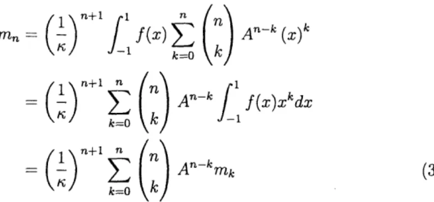
Recall that we are interested in the moments of the problem in the original domain. However, currently we have D set of moments, each of which corresponds to the moments of one of the sections. Therefore, using Equations 3.7 and 3.11, any arbitrary moment m, for any partition between [ai, bi] in the original domain s can be written
bi
f1(x)
+
a dx-1 I I
Sf(x)
(x + 1 + nain)" dx
S n 1 f(x)
(x +
A)" dxUsing this can be rewritten asthe Binomial Theorem, Using the Binomial Theorem, this can be rewritten as
=
()n+1f()
A
n-k
A )-k
(x)d
= n 1 ) Ak==
(1)n+n
An-kmk
(3.18)
k=o k
Note that rn, in Equation 3.18 is a moment in the original domain, while the mk are moments in the transformed domain. Hence, the nth moment in the original domain is just a linear combination of all the moments from 0 to n in the transformed domain. Using Equation 3.18, the moments of the original domain on each of the sections [ai, bi] can be calculated. The moments on the full domain are obtained simply by summing up all the corresponding moments from each partition to obtain the full moments on the original domain.
3.9
Brief summary
Figure 3-3 provides a summary of the whole process. Consider the function on the top left corner. This is the function whose moments we are interested in. We partition the function domain into D partitions, and map each partition to a normalized scale. For each partition, we write linear, and semidefinite constraints. There are also coupling conditions between the partitions. We solve the optimization problem which results in D sets of moments that correspond to each partition. These are combined in a particular fashion to give us the moments of the original domain.
3.10
Higher order ODEs
The formulation above is easily expanded to higher dimensions as well. In higher dimensions, more boundary conditions are required to specify a particular solution of
1
-1
Coupling cond. in the linear constraints
/I
Solve optimization problemCombine
Figure 3-3: Brief Summary of Algorithm - The original domain is partitioned and each partition is transformed to a normalized scale. Using the adjoint operator linear constraints are generated. Coupling conditions between partitions, and SDP con-straints are also written and the optimization problem is solved. Finally, the original moments of the system are recovered by combining the moments corresponding to each partition.
the ODE, and therefore, there are more unknowns in the optimization problem.
3.11
Implementation for testing purposes
Lets consider the one-dimensional adjoint equation,
xa(Obu) = Jp(bU )(xaqs)dx
- Jo(abu)4dx
ub-
l
ap
"+
)k+1ub-k
(k- 1) Ia n+ (-)b+IUb-1
Ian +
(-1)bu
fn Ubdx.
Given any derivative operator of order b, and a coefficient in front, by applying the adjoint operator, it is decomposed into b boundary conditions, and one moment of the solution. The moment number is a function of the coefficient, the test function, and the order of the derivative operator; however, all these can be automated. Hence, instead of explicitly writing equations for any particular problem, a program was developed in Matlab to automatically generate the matrices that can be inputted into a SDP solver.
Methodology
The linear constraints corresponding to each partition can be written as
Aii = bi, V i 1. .. D,
where Ai, xi and bi are generated dynamically as described below:
Sxzi Vector : The xi vector contains all the boundary conditions and the
mo-ments for the ith partition. The size of the vector is determined by the highest derivative operator in the differential equation. Some of the derivative condi-tions might be known, and therefore, there might be some known variables in
the vector. The general structure of xi is
* Ai Matrix : The matrix, Ai, will contain the coefficients corresponding to the
variables in the optimization problem for a particular partition. Each row of Ai would correspond to a particular test function, 0. Given a particular (XzaUb),
the coefficients in Ai are calculated, and thus updated.
* bi Vector : The bi vector contains the terms
f
2 f (c+ + ai) ¢ integrated withrespect to x.
Additionally there will be coupling conditions between the partitions. Hence some variables in xz = xi+l. We would also generate the SDP constraints for each partition from the elements of xi.
ub-1l(k
2)
ub-l(ki)
ub-2(k
2)
ub-2(kl)
u'(k
2)
u'(ki)
u(k
2)
mo u(ki) Tn1 mN m2NChapter 4
Numerical validation
The new methodology was applied to a few test cases. A wide range of ODEs were used as test examples. Some of the examples are simple ODEs, while others are more interesting such as the Bessel function, and Legendre polynomials. ODEs with known solutions were used as test cases. This allowed us to compute the actual moments analytically, which could then be compared with the solution from the optimization problem for accuracy.
4.1
Examples
-
plots and error plots
The objective of the solver in most of the one-dimensional cases was to minimize the value of 8mo +3m, of the solution of the ODE. This is an arbitrary function chosen for no particular reason. Recall that mo and m, are moments of the solution as defined in Equation 2.2.
By minimizing and maximizing the objective in the optimization problem, we would obtain a lower and upper bound for the objective function. For each problem, the bounds were initially calculated using no partitions and then using 2, 4, 6, 8 and 10 partitions. As well, the highest degree of the test functions N was incrementally changed from 2 to 10 for all the test cases. For example, N = 4 implies that the test functions used for generating the linear constraints were 1, x, x2 , x and x4.
the differential equation
u" + 2u' + 401u = 401, u'(1) = -1, u'(1) = -6.872,
using no-partitions and 4 partitions respectively.
Table 4.1: Lower and ODE 'u" + 2u' + 401u
Upper bounds on the value of 8mo + 3ml of the solution of
= 401, u'(1) = -1, u'(1) = -6.872' using no-partitions
N
Lower Bound
Upper Bound
3 8.58782387252627 331.2287657117187 4 8.60087181588462 12.41832038791917 5 9.35163490722703 11.31012965523155 6 9.35367056758392 10.13361730268152 7 9.41130776281981 10.00834412042844 8 9.49422948153400 9.83683698700403 9 9.49724559720386 9.80643867214983 10 9.55660706980515 9.80654282114558
In this case, the analytical value of the objective is 9.69401509901859. We see that by increasing N, the lower bounds and upper bounds converge towards this value. The bounds obtained in the 4 partitions case is closer to the objective value, and the gap between them is smaller. Hence, this gap is an indication of the accuracy of the bounds computed. Lower the gap, better the estimate for the value of the objective function. Therefore, Figures 4-1 to 4-7 show the plot of the solution obtained analytically, and the gap between the upper and lower bound for various test cases. In some cases, the
Table 4.2: Lower and Upper bounds on the value of 8mo + 3ml of the solution of ODE 'u" + 2u' + 401u = 401, u'(1) = -1, u'(1) = -6.872' using 4 partitions
N
Lower Bound
Upper Bound
3 9.45099457753055 9.91766331785804 4 9.55343533597745 9.81232591136663 5 9.60923930097504 9.75148420145830 6 9.67541139308819 9.71141601527514 7 9.68830926142656 9.69884262144618 8 9.69332268823363 9.69474744135362 9 9.69386826616983 9.69417842220312 10 9.69399830895136 9.69403139077513
no-partition case does not find an upper bound because the problem is unbounded. In such cases, the upper bound was set to be 1000 as this is substantially greater than the value of objective function.
4.1.1
ODEs with closed form solution
Figures 4-1 through to 4-5 demonstrate the application of the methodology on various ODEs with a closed form solution. Although simple, they give a very good insight on the behaviour of the algorithm.
4.1.2
ODEs with no closed form solution
Many ODEs do not have an explicit closed form solution. Rather, the solution is written as a summation of infinite terms. Figure 4-6 shows a practical application by finding the variance of the solution of the Bessel differential equation, z2u" + u' +
(9X2 - 1)u =:: 0. The solution of this ODE is the J (3x) function. The first and second moments were calculated, and the variance was calculated by m2 - m . Figure 4-7 is
a solution to the ODE (x2 - 4)u" + 3u' + u
= 0. This is an interesting example, and the reasons for this are discussed in Section 4.2.1.
4.2
Discussion
4.2.1
Accuracy of solution
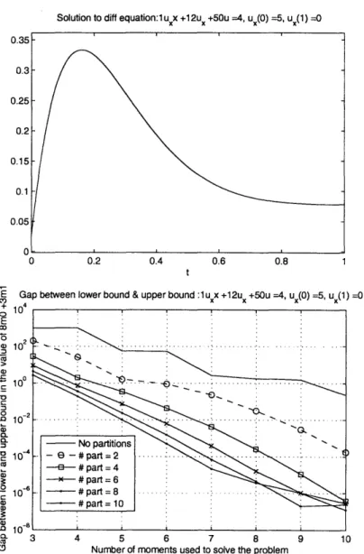
Consider the error plot in Figure 4-1. The gap between the lower and upper bound becomes small (10-6) if we take a large value of N, even for the non-partition case. However, all the partition cases seem to have similar gaps ( 10-10) between the upper and lower bounds of the solution. The solution of this ODE is a smooth function that is monotonically decreasing in the domain [0, 1]. In the case of the ODE, u" +
3u' - 4u = 0, Figure 4-2 indicates that the non-partitioned case does not achieve as much accuracy as the various partitioning cases. Moreover, we see a little bit of segregation between the various partitioned cases, for lower values of N used. The
Solution to diff equation: 1 uxx +3ux +-4u =0, ux(0) =-1, ux(1) =0
0 0.2 0.4 0.6 0.8
Error in solution to diff equation:1uxx +3ux+-4u =0, ux(0) =-1, ux(1)=0
3 4 5 6 7 8
Number of moments used to solve the problem 9 10
Plot and error in the solution to ODE u" + 12u' + 50u = 4, u'(0) =
Figure 4-1:
![Figure 3-1: Partitioning the domain into D partitions. Each partition is mapped on to a new domain [-1, 1]](https://thumb-eu.123doks.com/thumbv2/123doknet/14752794.580999/35.918.163.744.109.467/figure-partitioning-domain-partitions-partition-mapped-new-domain.webp)