The diurnal tides on the Northeast continental shelf off North America

THE DIURNAL TIDES

ON THE NORTHEAST CONTINENTAL SHELF OFF NORTH AMERICA

by

PETER REID DAIFUKU B.A., Swarthmore College

(1978)

SUBMITTED TO THE DEPARTMENT OF EARTH AND PLANETARY SCIENCES

IN PARTIAL FULFILLMENT OF THE REQUIREMENTS FOR THE

DEGREE OF MASTER OF SCIENCE IN PHYSICAL OCEANOGRAPHY

at the

MASSACHUSSETTS INSTITUTE OF TECHNOLOGY September 1981

OMassachussetts

Departmi Earth and Planetary Sciences August 1, 1981 Certified by

Zq

MASSACHUSETTS INSTiTUTE

WiTHFR

I

19,

FRO31

MIT LIBRA

'

2

THE DIURNAL TIDES

ON THE NORTHEAST CONTINENTAL SHELF OFF NORTH AMERICA

by

PETER REID DAIFUKU

Submitted to the Department of Earth and Planetary Sciences on August 1, 1981 in partial fulfillment of the

requirements for the Degree of Master of Science in Physical Oceanography

ABSTRACT

The diurnal tides are presented on the Northeast continental shelf off North America, from Nova Scotia to Cape Hatteras. Available current meter data were analysed using the response method, which calculates the tide as an empirical modification to a reference time series, here the equilibrium tide. The results are tabulated for the K1 and 01 diurnal tides, and the M2, S2 and N2 semi-diurnal tides, along with an estimate of the 95% confidence limits. Maps of the K₁ tidal ellipses, as well as maps of the K1 currents are presented for different phases of the tide. In order to complete the picture of the tide, I obtained analysed coastal sea level and bottom pressure data, and also present a cotidal-corange map of the K1 tide.

I have attempted to model the observed K1 pressure field by calculating the allowed free and forced waves for a series of cross-shelf

sections, using the linearized inviscid shallow water equations and the assumption of a two-dimensionnal straight shelf. The theoretical

solutions are then fitted to the data using a least squares method. The model results confirm that the diurnal tide is composed of both a Kelvin wave and a shelf wave, with the Kelvin wave dominating the pressure

field, and the shelf wave dominating the currents. The free waves account for roughly 99% of the variance of the difference of the observed pressures and the calculated forced wave, but unfortunately some of the observed features are not accurately reproduced . Possible improvements would include the addition of bottom friction and a better description of

long-shore topography, especially as concerns the transition from the Gulf of Maine to the New England shelf.

Thesis Supervisor: Dr. Robert Beardsley Title: Senior Scientist

Acknowledgements

Much of this work was done in cooperation with B. Butman and J. Moody of the United States Geological Survey (USGS), and with W. Brown of the University of New Hampshire (UNH). Butman and Moody are developing a description of the semi-diurnal tide in the same area and Brown is examining sea surface tides as determined by bottom pressure sensors and coastal tide stations.

I would like to thank my advisor, Bob Beardsley, for his support through this year. Ken Brink gave some valuable suggestions on the manuscript. Carl Wunsch supported me for a semester through an ONR contract, Sea Grant and the Education office at the Woods Hole Oceanographic supported me for the remainder. Many thanks to the USGS for their support in computer time, without which the theoretical analysis and much of the data analysis could not have been done; and to the people in Graphics at the Woods Hole Oceanographic Institution who produced many of my figures. Finally, thanks to Anne-Marie Michael for the final typing touches.

Table of Contents

Abstract ... ... Acknowledgements...

Introduction ... Data Analysis Methodology ...

Analysis Methods... Noise Determination ... The Observed KI Tide and Tidal Curre A Theoretical Model for the K1 Tide. Procedure ... Derivation of Governing Equation The Free Wave Solutions...

Forced Wave Solution Results... Model to Data Fit... Results of Fit... Discussion... Conclusion... Appendix ... ... References... Biographical Note... ... 2 ... 10 nts ... 15 ... 25 ... 25 s... ... 25 ... 27 ... 28 ... 30 ... 41 ... 42 ... ,,...,o,55 ... 57 ... 59 ... 95 ... 97 ... ... ... ... ... ... o.. ... .... o ... ... ... ... ... ... ... ... ...

I) Introduction

Coastal tides are an important phenomenon, accounting for a significant ammount of the ocean's energy on the shelf. Their signal dominates the sea level and current spectrum for frequencies of order one cycle per day or greater, making the determination of other physical processes at those frequencies difficult. Conversely, their high energy implies that shelf currents can be strongly influenced by the tides, both through tidal rectification and tidal friction. Tidal currents also play an important role in mixing, material dispersion and sediment transport.

I present here a study of the diurnal tide from Nova Scotia to Cape Hatteras. The southern point essentially marks the boundary between two different tidal regimes, a strongly semi-diurnal regime to the north and a more diurnal regime to the south. The northern limit marks the end of the

Gulf of Maine-Scotian shelf region. The recent proliferation of current meter and pressure gauge recordings on the shelf permits a thorough study of shelf tides in this area. Figure 1 shows the location of our current meter and pressure stations, with a perhaps (?) coincidental concentration

around Woods Hole.

Part II outlines the methods of analysis, including the estimation of 95 percent confidence limits, while Part III displays the result of that analysis for the K₁ tide, with a cotidal-corange map for the surface tide, and a series of maps of the velocity components for different phases of the tide. Part IV presents a simple model to fit to the K₁ pressure data along different cross-shore transects. I show that, to a first

6

approximation, the data can be explained by a combination of a Kelvin wave and a shelf wave, and a third wave forced by the equilibrium tide. Part V offers some possible mechanisms by which the fit between the data and the calculated waves could be improved.

II) Data Analysis Methodology

A) Analysis Methods

The analysis of tidal data differs from standard time series analysis, since the high energy content of the important tidal lines precludes a naive use of Fourier Transforms, due to severe leakage to adjacent bands. The deterministic nature of the astronomical forcing means that the tidal frequencies are well known, however, so that the appropriate use of this knowledge can greatly simplify the time series analysis.

There are two methods principally in use to analyse tidal data. The harmonic method performs a Fourier analysis at selected tidal frequencies. Various corrections are then applied to correct for the fact that the main tidal frequencies are not the harmonics of a fundamental, as called for by simple Fourier theory. The vade mecum of harmonic analysis is the 1941 manual of Paul Schureman. A modern variant is the use of FFT routines on today's high speed computers. Since the frequencies are no longer exactly aligned with the tidal frequencies, leakage is particularly severe, so that this variant is best used on long time series (i.e. a year or more).

The second principal method was developed by Munk and Cartwright (1966). Known as the response method, it calculates the tide as an empirical modification to a known input potential. More specifically, the

predicted tide np can be written

np(t)= E ws V(t- s )

where V is the input potential, and the weights w_s are chosen such that np is a least-squares fit to the actual data. Following convolution theory, ws can then be thought of as the impulse response of the sea surface (or currents) at that point. The choice of a suitable input potential is a matter of convenience. If there is a nearby location where the tide is accurately known, then the predicted tide for that location can be used as the input potential. On the other hand, the equilibrium tide is easier to produce, but may provide a less accurate solution. The equilibrium tide is the theoretical tide one would calculate for a non-inertial homogeneous ocean on a smooth sphere, and can be calculated directly from the known astronomical constants. The various frequencies of the harmonic method are selected based on an expansion of this

potential.

The response theory is intellectually more appealing than the harmonic method. The latter uses a knowledge of the more important lines, while the former takes into account the entire equilibrium potential.

Also, the use of Fourier analysis for the harmonic method implies that certain record lengths are better than others for resolving a given line. As a corollary to this, a minimum of fifteen days of data is necessary to resolve the major lines (M2, S2, N2, K1, 01). The response method has no such drawbacks; in particular, the calculation of a

predicted tide should be more accurate, since there are no assumptions made as to which frequencies are important. In addition, the response method has the added attraction of incorporating some physics into the otherwise purely numerical analysis: namely, that the response of a given location is directly related to that of a nearby site, or to the equilibrium tide. In practice, it turns out that both methods yield fairly similar results, given an adequate record length. In particular, we lose some of the advantages of the response method by requiring it to calculate given harmonic constituents, rather than a full predicted tide.

Because of its convenience, we chose to use the response method.

B) Noise Determination

Following Munk and Cartwright (1966), I plan to use the noise to signal ratio a as a basic parameter of the quality of the calculation, such that

02= variance of noise/ (2L x recorded variance), where

L= length of series in lunar months,

and the variances are averaged over the appropriate tidal band. This definition was used by Munk et al. (1970), and is a slight variation on the original formula proposed by Munk and Cartwright (1966), where L was replaced by p, the number of independant segments over which the variances were averaged. In such a way, band averaging can be substituted

for piece averaging: following standard spectral analysis, a month of data gives a maximum resolution of one cycle per month, or, using the

language of tidal analysis, resolution of tidal groups. The major tidal lines fall within separate, distinct groups, with the exception of the S₂ and K₂ lines, which are separated by one cycle per year. Thus L can be thought of as the degrees of freedom associated with separating

the various tidal groups. The final error estimate will be valid for a given band, diurnal or semidiurnal, rather than for a specific line. This assumes that most of the residual variance is due to baroclinic tides, rather than white noise, as explained in Munk et al. (1970). Hence the

error estimates will be conservative estimates for the major lines.

In order to calculate the noise variance, I calculate a predicted tide, creating a tidal time series to match the inputted data. If I subtract this predicted series from the observed one, I then get a residual time series, which can easily be analysed spectrally, as it has a nearly normal distribution. To obtain the noise variance, I then average over each tidal band, defined as m cycles/lunar day + 4.5 cycles/lunar month, where m is the species number. Note that this process

does not entail Fourier analysis of the raw data, so that I avoid having to deal with the strong leakage associated with the very energetic tidal

signals.

The leakage problem also makes it undesirable to calculate the recorded variance directly. Instead, I will assume that the recorded variance is the sum of the prediction variance, and of the residual variance. I have just outlined how to calculate the latter; the program

calculates the former, which is basically the covariance with 0 lag of the predicted diurnal or semi-diurnal tide with the observations.

Given a, Munk and Cartwright (1966) calculate probability distributions for the amplitude and phase of the admittance, respectively:

p(p)=(o/a 2_)exp(-(p-1) 2_/2G2_)(exp(-p/a 2₎

0(p/a 2)), p(o)=(2n)-lexp(-1/2a2)(1+F(cose/a)), where F(x)=x exp(x2/2)f exp(-t 2_{/2) dt,} -x with -x P= R/R, e= 5 - true phase.

- denotes estimated quantities, R=true admittance. These equations are integrated with respect to p and e, with limits of integration determined by the condition that 2.5 percent of the distribution lie on either side of the integrated span. Plotting these limits as a function of a gives figures 2 and 3, which reproduce Munk and Cartwright's (1966) figure 16.

The pressure data were analysed at the UNH using the harmonic method. Note that the error analysis performed at the UNH assumes that the tidal residual is mainly white noise. This means that errors in neighbouring constituents are assumed independent of each other, so that error bars for the major tidal lines of each band tend to be lower than they would

be using my procedure. In terms of consistency, all current data has been processed using one assumption, all pressure data the other. Thus, while the result is not as satisfactory as if one single method had been used, comparison among current stations or among pressure stations is still meaningful.

FIGURE 2 95% confidence limits for estimated coefficient - true coefficient

.0

G

FIGURE 3

0T

-

00 0.70 '.0 i.5 2.00 2.50

95% confidence limits for 6 = true phase - estimated

phase

95% onfience]imis fo 6 tu pae etmae

III) The Observed K1 Tide and Tidal Currents

The results of the analysis are tabulated in tables Al and A2, and maps are shown in figures 4 to 11.

a) cotidal map

Figure 4 shows the data used to contour figure 5. The object was to draw as smooth a representation as possible, given the 95 percent confidence limits which accompanied most of the UNH data. As such, it is only one of several possible mappings, the one which seemed most logical

and plausible. Offshore, there is a sweep of the tides from North to South, generally conforming to the picture of the global K1 tide as we know it. (See figure 6, reproduced from Defant (1961)). I also took into consideration the presence of an amphidrome near Sable Island, as observed in most global models. Note the appearance of a virtual

amphidrome located South of Cape Cod, and a severe twisting of the cotidal lines over the Northeast Channel. The highest amplitudes are around fifteen centimeters and are found in the Gulf of Maine, the lowest are around seven centimeters, in the vicinity of Cape Cod.

b) velocity maps

Outside of the bottom boundary layer, the velocities show only a small phase and amplitude shift with depth, confirming the barotropic nature of the tides. Thus, in figures 7 to 11, we show the maximum

currents within a given mooring, since these should errors, and still should be characteristic of the 1

shows representative current ellipses, while figures K₁ currents at various phases of the tide.

In general, the current ellipses are aligned topography, with the maximum currents occuring near There is only a slight cross-shelf phase shift. The observed were within the Gulf of Maine, the largest Shoals. have the ocation. 8 to 11 smallest Figure 7 show the

with the local the shelf break. smallest currents south of Nantucket

K1 Tide, Greenwich Hours

4 4

S 0 S 0 0 0 0

IV) A Theoretical Model for the K1 Tide

A) Procedure

I attempt here to develop a theoretical model which will reproduce in part some of the observed features of the K1 surface tide and currents.

I first find the free and forced solutions to the shallow water equations for realistic cross-shelf profiles. I have chosen four such profiles, where I had at least three pressure stations more or less aligned in the cross-shelf direction. These sections are identified by the dashed lines in figure 1. The first one uses the Nantucket Shoals Flux array as a basis, and stretches South of Cape Cod. The second one starts from Long Island, the third from Atlantic City. The fourth stretches across the Gulf of Maine and Georges Bank. I then fit the solutions to the pressure data along those sections using a least-squares procedure. I chose to fit to the pressure data only, since it is inherently cleaner than current meter data. Much of what follows is based on Munk et al. (1970), and Cartwright et al. (1980).

B) Derivation of Governing Equations

Start from the linear shallow water equations, u*t*-fv*=-g( n*-nE*)x*

v*t*+fu*=-g(n*-nE* )y* (4-1)

with nE* a forcing term, here the equilibrium tide. In a right-handed coordinate system, take the y axis to be aligned with the coast, and x* equal to 0 at the coast, positive offshore. Assume that the depth is a function of offshore distance only,

h*=h*(x*) (4-2)

I next scale the terms by the following representative quantities U ,v~U,

at-f, aayLa _- 1 h-H, n -fUL/g,

where L is some estimate of the shelf width and H is some estimate of the offshore depth. I chose L=200km, H=2400m for sections 1,2,3, and L=500km for section G. Then system (1) becomes

u t-v =-(n -nE )x, v't+u _{=-(n -nE )y,} D2n t+(hu)x+(hv)y=O,

(4-3a) (4-3b)

(4-3c)

where

D2=f2L2/gH=(L/Rossby radius of deformation)2

Now assume propagating solutions proportionnal to exp i(ky-wt). (4-3a) and (4-3b) can then be solved for u and v to get:

u=(iw(n-nE)x-ik(n-nE))/(₁-w2), v=(-wk( n-n E)+( n-nE )x) / ( 1 -w 2 ).

Introducing these into (4-3c) yields a single governing equation for the free surface elevation

(hnx )x-(k2h+khx/w+(l-w2)D2) n= (hnEx)x-(k 2_h+khx/w)nE

Free solutions are obtained by solving (4-4) with nE set to 0.

C) The Free Wave Solutions

I wish to solve

(hnx)x-(k2h+khx/w+(1-w

2_)D2)n=O with the appropriate boundary conditions

hu=O at x=O,

whnx-khn=0 at x=O, and

->O0 as x-+ o.

(4-5a) can be reduced to a system of two coupled first order equations by setting

1=n,

Y₂=hnx,

so that (4-5a) becomes

(4-6a) (4-6b) Y2'=(k 2h+khx/w+(1-w2_)D2_)y1. (4-4) (4-5a) (4-5b) (4-5c)

(4-5b) becomes

Y₂-khY₁/w=O at x=O. (4-6c)

The appropriate deep sea solution to (4-5a) when h=1 for x>1l is n=exp-(k2+(1-w2 )D2 ) 1/2x,

so that the appropriate boundary condition at x=1 is

Y1'+(k 2+(1-w 2)D2)1/2Y1=0 x=1. (4-6d) Equations (4-6) can easily be solved numerically for realistic profiles. Huthnance (1975) showed that for the case of a monotonic depth profile, the free solutions for sub-inertial frequencies consist of a Kelvin wave,

and a series of shelf waves, all of which propagate phase with shallow water on the right, and decay exponentially offshore. The first shelf wave mode has one zero crossing, the second two, and so on. For a given wave number k, higher modes have lower frequencies, and generally, for a given frequency and mode number there are two solutions to the dispersion relation, with phase propagation in the same direction but with the energy propagation of the shorter wave in the opposite direction. Here, the frequency peak of the second mode lies below the K1 frequency, so that only the Kelvin wave and the first shelf mode exist as free waves.

D) Forced Wave Solutions

Now solve equation (4-4)

(hn x ) x - ( k 2 h +k h x /w+ (1-w2 ) D2 ) n= (hnEx)x-(k2_h+khx/w)nE

into account the self attraction of the tidal bulge and the deformation of the yielding sea bottom. nE* is then

nE*=.69V/g

where V is the equilibrium tidal potential. Now V sweeps across the earth from east to west every 24 hours for the diurnal tide, or with a non-dimensionnal wave number

a=L/(r cose)

with r radius of the earth and e latitude. Relative to a coastline at an angle 0 from true North, I can write

nE=ex_p i(aEx+BEy-(wt-GE))' where aE=-a cos Q,

BE=-a sin 4,

GE= West longitude of x=O. Here,

c=4.08 x 10-2 for sections 1,2,3, a=0.12 for section G, 0=45° for all sections,

Dimensionnaly,

nE*(O)=HE where

HE=9.68cm for profiles 1 and 2, =9.55cm for profile 3,

=9.74cm for profile G.

The solution to (4-4) can be written as

Substituting (4-7b) into (4-4) gives

(hRx)x-( E2_h+aEhx/w+(1- 2_{) D}2_)R=(1-w 2_{) D}2_{nE (4-7b)} I need, once again, u=O at x=O, or

wRx_-ER=O, x=O, (4-7c)

and for xioe, we need nF-nE, or R*O as X-m, or in equivalence to (4-6c)

Rx+(a2+(1-w2)D2)1/ 2R=O x=1 (4-7d)

This system of equations is easily solved numerically, involving only a slight modification to equations (4-6), namely the inclusion of a near constant term on the right hand side of (4-7b).

E) Results

Figures 12 to 19 show the solutions to the free and forced problems. Only the longer of the two first mode shelf waves are displayed, as the velocities associated with the shorter waves were unreasonably high in the subsequent least squares fit. The velocity profiles are obviously more sensitive to small variations in cross-shelf topography than the elevation profiles. Since there is a good deal of approximation involved

in the determination of the topography, this is clearly another reason why the model wave fitting to data should be based on pressures only.

Table I below summarizes the long-shore dimensionnal characteristics of the waves for each profile.

Table I Profile 1 Profile 2 Profile 3 Profile G Kelvi n k=-5.2x10-4/km x=11979km c=501km/hr k=-5.2x10-4/km x=12106km c=506km/hr k=-4.7x10-4/km x=13312km c=556km/hr k=-4.8x10-4/km x=13022km c=544km/hr Shelf k=-1.4x10-2/km x=462km c=19km/hr k=-1.3x10-2/km x=50lkm c=21km/hr k=-1.3x10-2/km x=493km c=21km/hr -3 k=-2.6x10-3/km x=2407km c=101km/hr Forced k=BE=-5.2x10- 4 /km x=43558km c=1820km/hr SAME AS PROFILE 1 SAME AS PROFILE 1 SAME AS PROFILE 1

Note that characteristics of the three waves are fairly similar for profiles 1 to 3. In the Gulf of Maine, h

Kelvin and forced waves are similar different, with a wavenumber about four other profiles. Clearly, then, the tran Gulf of Maine to beyond is non-trivial. shows that a sustained displacement of phase of order (kx₁)2, where _xl displacement. For the Gulf of Maine, k2x 2 is roughly .02. I thus expect from the change. owever, whi the shel times smal sition of t

For the Kel the coastli

is the x1 is ro

le wavenumbers for the f wave is radically ler than that for the ie shelf wave from the vin wave, Miles (1972) ne induces a change of

magnitude of the ughly 300km, so that the Kelvin wave to propagate Gulf of Maine onto the New England Shelf without noticeable

C) o \)/

0

IN.)

Profile 1: Free Waves Thick Line = Topography

Profile I: Free Waves

LO)

I0.00 25.00 50.00 75.00 100.00 125.00 150.00 175.00 2b6.00

DISTANCE FROM COAST, KM

o

O T1

0 u

= Kelvin Wave

10.00 25.00 50.00 75.00 100.00 125.00 150.00 175.00 206.00

DISTANCE FROM COAST, KM

6 43 U i 0 \ o I

o

_E

_o"

-u

Profile 3: Free Waves Thick Line = Topography

0

o I

0.o00 25.00 50.00 75.00 100.00 125.00 150.00 175.00 20 00

DISTANCE FROM COAST, KM

0

Profile G: Free Waves

T1o

E

o

o

Thick Line = Topography /

. 0

o

bO VO

C; 1

.00 50.00 100.00 150.00 200.00 250.00 300.00 350.00 400.00 450.00 500.00

DISTANCE FROM COAST, KM

O 0 0 - 0

to

Profile 1: Forced Waves II I I I 00

C00.00 25.00 50.00 75.00 100.00 125.00 150.00 175.00 20%00

DISTANCE FROM COAST, KM

O O

0 Profile 2: Forced Waves _C

O I 0 00 (0 L0 0 0 0 - 0 O 00.00 25.00 50.00 75.00 100.00 125.00 150.00 175.00 2 0 :00

DISTANCE FROM COAST, KM

0 0

0 Profile 3: Forced Waves C

0 CO

DISTANCE FROM COAST, KM

a

0D 0

o Profile G: Forced Waves 0

0 0 ILA 0 o Li.L a 0 Q _oa 0 ao .00 50.00 100.00 150.00 200.00 250.00 300.00 350.00 400.00 450.00 500."

DISTANCE FROM COAST, KM

F) Model to Data Fit

Since the transition of the shelf wave from the Gulf of Maine to the New England Shelf is so problematic, I chose to limit attention to sections 1 through 3 for the main least squares fit. The Kelvin and shelf waves are being fit to the data, the forced problem being totally determined. I regard the amplitudes and phases of the Kelvin and shelf waves to be fixed, so that the only difference from profile to profile is a propagation term, exp(iky). The residual, E, can be written as

E= (Di-Fi-Ki-Si) (Di-Fi-Ki-Si

)*

where i=1,11 numbers stations along profiles 1,2 or 3.

Di are the various data points, taken from table Al, Di=Hi exp iGi,

F i=AF exp i(longitude)=forced term, AF=HE(1+Ri) (see Sec. IV-D),

Ki=AKHKi exp i(kKy+eK)=Kelvin wave, Si=ASHSi exp i(kSy+eS)=Shelf wave.

HK, HS are the normalized sea surface heights calculated previously. AK, AS, eK, e_S are the unknowns; y is the distance between sections and is 0 for profile 1; k is the average of the wavenumbers for the profile through the station and the profile upshelf before it. I then take partials of E with respect to AK cos eK, AK sin eK, AS cos eS, AS sin eS and set them to 0. This gives me a system of four

42

G) Results of Fit

Results of the pressure data fit are displayed in table II. The eleven stations used for the fit are: NSFE1, NSFE2, NSFE4, NSFE5 for profile 1; A4, MESA5 and 1-2-19 for profile 2; Atlantic City, MD, MB and MC for profile 3. Variances are calculated for all eleven stations. "Data variance" is actually the variance of the observed tide minus the forced response, and is thus the variance that has to be reduced by the

43 Table II Profile 1 y=O Kelvin Shelf amp=13.2cm ph.=208 amp=2.6cm ph.=-82 0 amp=7.9cm ph.=70 Forced Obs. Calc. NSFE1 H,G 6.5,173 8.6,177 (cm,deg) NSFE2 7.3,173 8.8,174 NSFE4 8.1,177 8.7,169 NSFE5 8.6,175 8.8,167 Data variance=1933.2cm2 Kelvin variance=1841.2cm2 Profile 2 y=-l60km amp=13.2cm ph.=2130 amp=2.6cm Profile 3 y=-380km amp=13.2cm ph.=219 amp=2.6cm ph.=197° amp=8. O0cm ph.=380 amp=8. 1cm ph.=72 0 Obs. Calc. ph.=740 Obs. Calc. Atl. Cit. 8.4,168 7.4,168 MESA5 8.3,175 7.9,172 1-2-19 6.3,181 7.6,170 10.7,181 10.6,188 MD 10.3,182 8.9,185 MB 9.0,176 8.0,182 MC 9.0,180 7.6,181 Residual variance=22.lcm2 Shelf Variance=11.3cm2

Using the calculated amplitudes and phases for n, the associated

cross-shelf u and along-shelf v velocities can be calculated for the Data

44

current meter stations which lie along the various profiles. These composite velocities are listed in Table III.

Table III Profile 1

Station u v

Amp. Phase Amp. Phase

NSE 1.5 -133 4.7 100 NSFE1 2.1 -148 4.6 99 NSFE2 2.1 -145 3.7 101 NSFE3 2.3 -150 3.2 103 NSFE4 2.3 -152 3.1 101 NSFE5 2.3 -155 3.0 100

Variance Kelvin=13.8cm2/sec2 Variance Shelf=72.8cm2 /sec2 Variance Forced=11.4cm2/sec2

Amp. .6 3.4 3.8 .4 Kelvin=5.3cm2/sec2 Shelf=73.Ocm2/sec 2 Forced=3.2cm2/sec 2 Amp. .2 .8 1.7 Kelvin=8.2cm2/sec2 Shelf=45.2cm2/ s e c 2 Forced=4.6cm2/sec 2

From the above, c while the shelf wave shelf wave velocities three different waves

learly the Kelvin wave dominates the pressure signal, dominates the velocity field. The dominance of the is apparent in the data: despite the combination of with very different characteristics, the cross-shelf Profile 2 Station Phase -63 -61 -60 -59 CMICE MESAS NES762W NES763W Variance Variance Variance Amp. 3.4 4.3 4.2 .8 Phase -143 -150 -150 41 Profile 3 station Phase -77 112 117 EGG MB MF Variance Variance Variance Amp. 4.9 2.5 2.7 Phase 22 29 31

of the velocities is cotidal-corange map,

remarkably coherent. for comparison with

Figure 20 figure 5. progression of the Kelvin wave offshore, while nearshore

with the shelf wave "traps" the phase lines virtual amphidrome 120km from Profile 1, and Profile 3. While similar patterns can be seen not reproduced. In particular, the virtual shifted westward in figure 20. Figures 21 i

to the c the hint in figure amphidrome to 23 the interaction ast. There is a f another beyond 5, the detail is of figure 5 is compare the suitably rotated velocities for each profile, with the observed velocities on right, and the corresponding predicted velocities on the left. In these figures, the ellipses are oriented so that the vertical is North. Apart from Profile 1, the calculated velocities are embarassingly different from the observed ones, and in most cases within the 95 percent confidence limits.

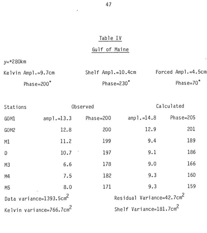
I used a similar scheme for the Gulf of Maine. Propagation from Gulf to the New England Shelf was assumed to have little effect on Kelvin wave phase speed, allowing the Kelvin wave phase to be set (kKy+eK). The shelf wave amplitude and phase were allowed to vary. unknowns in this case are thus the amplitude of the Kelvin wave, and

and phase of the shelf wave. The D, M3, M4 and M5. The results are

seven stations used were GOM1, displayed below. structure predicted shows Note the the the all true not lie the the as The the amplitude GOM2, M1,

Table IV Gulf of Maine y=+280km Kelvin Ampl.=9.7cm Phase=200° Stations GOM1 GOM2 ampl.=13.3 12.8 M1 11.2 D 10.7 M3 6.6 M4 7.5 M5 8.0 Data variance=1393.5cm2 Kelvin variance=766.7cm2 Shelf Ampl.=10.4cm Phase=2300 Dbserved Phase=200 200 199 197 178 182 171 Forced Amp Ph a Calculated ampl.=14.8 Phase 12.9 9.4 9.1 9.0 9.3 9.3 Residual Variance=42.7cm2 Shelf Variance=181.7cm2 1.=4.5cm se=700 =205 201 189 186 166 160 159 ( 3

Table IV (cont.) Velocities station Amp. GOM1 GOM2 D K Variance Variance Variance .3 .4 2.8 3.6 Kelvin=69.8cm2/sec2 Shelf=90.2cm2 / s e c2 Forced=24. lcm2/sec 2

As can be seen, the the other profiles. velocities. Despite compare quite well.

Phase -74 -92 -172 -162 Amp. 3.8 3.2 4.9 5.0 Phase 49 52 83 97

residuals are proportionately much greater than for Figure 24 compares the observed to the calculated the poorness of the pressure fit, the velocities

DISTA NCE

ALONG

SHORE,

km.

Predicted Co-tidal Map for Profiles 1 to 3. --- lines

Slines vertical lines of equal amplitude in cm of equal phase = location of profiles FIGURE 20 380 340 300 60 20 170 0 50 Q) 100 150 200

PREDICTED VELOCITIES

_{PRFILE I}

~Is

PREDICTED VELOCITIES

PROFILE

I (C1NT.)

0

PROFILE 2

4

PREDICTED VELOCITIES OBSERVED VELOCITIES

PRDFILE 3

PREDICTED

VELOCITIES OBSERVED_VELOCITIES

PRIFILE 9

FIGURE 24 z

V) Discussion

Despite the low residuals, the comparison of figures 5 and 19 shows that the fit is not as good as one could wish. In particular, the virtual amphidrome south of Cape Cod which seems to be caused by the Gulf of Maine is not described at all by the predicted fit. In addition, a quick glance at figures 21 to 24 will show that the worst discrepancies for the velocities also occur for profile 1, where the theory is unable to explain the relatively large observed currents. I tried pushing my simple theory to its limits: I included the short first mode shelf wave, but this did not lower the pressure residuals appreciably, and made the velocities too high. The amplitudes of the Kelvin and Shelf waves were also allowed to vary from profile to profile. In order to get a least-squares fit, the variation in the shelf wave amplitude from profile to profile became unrealistically large, indicating that there should be easier ways of improving the fit. There are two types of changes that could be

incorporated into the model. The first consists of improving on the physics, by incorporating new physical processes into the equations of motion. The second consists of dealing with long-shore variations in topography.

There are two physical processes that come to mind: baroclinic effects, and frictional effects. Baroclinicity is of secondary importance.

Huthnance (1978) shows that the effects of stratification are greatest at high wavenumbers. The frequencies for a given wavenumber are raised, so

Lines of constant velocity tend to tilt away from the vertical with increasing stratification, so that shorter waves may become bottom trapped. In light of this, there should be no great modifications to the model from the inclusion of stratification, especially since the shorter first mode shelf wave has not been included. Frictional effects are likely to be more important. Brink and Allen (1978), in the limit of low frequency shelf waves (w<<f), show that incorporating a linear friction term -rv/h(x) produces a cross-shelf phase shift, such that flow nearshore leads offshore flow. Mofjeld (1980) demonstrates similar behaviour for the Kelvin wave. Table II shows such a trend, with near-shore calculated phases higher than observed, and near-slope calculated phases lower than observed. Thus, if an extension of the Brink and Allen (1978) study were to yield similar phase shifts, we would see an improvement in the fit. In particular, the strong semi-diurnal currents on Georges Bank contribute to enhanced bottom friction in that location.

So far, the shelf has been assumed to be infinitely long, with no alongshore variations in depth. The various solutions then have been assumed to flow smoothly into one another, at least for profiles 1 through 3. Again, following Miles (1972), these assumptions are probably valid for the Kelvin wave and the forced wave, due to their very large scales. Hsueh (1980) shows that alongshore variations in topography tend to scatter the shelf wave into all possible modes at the same frequency. In addition, the scattering of the incoming wave produces a cross-shore phase shift downstream of the irregularity, the sign of which depends on the sign of hy. Here, where only the first mode is permitted, the scattering is

limited to forward scattering of the incoming wave, to backscattering into the shorter first mode wave, and, (e.g. Brink, 1980), to scattering into non-propagating higher modes. The phase shifts are likely to cancel each other out, over a long and varied length of coast line.

Finally, there is the transition problem from the Gulf of Maine to the New England shelf. This is likely to be an important consideration, since the cotidal map shows a significant effect of the Gulf on the New England shelf, in particular helping to define a virtual amphidrome. The problem

is not trivial, since it involves the matching of the shelf wave across the Northeast Channel to the north, and the Great South Channel to the south. At a more basic level, the Gulf of Maine is approximately 400 km long, or a fraction of the wave length of the shelf wave, so that the existence of the shelf wave in this context is in doubt. This is clearly an area for further study, possibly by a numerical model for the region.

VI) Conclusion

I have analysed available current meter data on the continental shelf from Nova Scotia to Cape Hatteras. I have tabulated the tides for five major lines, M2, S2, N2, 01 and K1 (see appendix). I obtained analysed pressure data for the same area, and examined the K1 tide in detail. Offshore, there is a general sweep of the tide from north to south. Near the coast, there is a virtual amphidrome south of Cape Cod. This amphidrome coincides with a zone of high velocities (- l0cm/sec). Current ellipses are generally aligned with the local topography.

(1980) we have gone one step further realistic profiles. A least squares despite its variance ir wave, there dominating The forced forcing, wh incoming de forced wave I have

by calculating wave forms for four fit to three of these shows that, shortcomings, the model can account for a good deal of the the K₁ pressure field. Clearly, in addition to the forced exists a Kelvin wave and a shelf wave, with the Kelvin wave the sea surface field, and the shelf wave the velocity field. wave is a first order local response to the gravitational hile the free Kelvin and shelf waves are a response to the ep sea tide, and a secondary response to the interaction of the

with the shelf.

outlined ways of extending our model, with the most likely improvements taking into account bottom friction and the transition from the Gulf of Maine to the New England shelf.

One would expect similar results to hold wherever D2=f2L2/gH is small enough. Huthnance (1975) shows that w is a monotonically decreasing function of D for a given k, and Buchwald and Adams (1968) show that for a

given offshore depth H there is a maximum allowed frequency wmax* If Wmax is less than wK1, then there will be no diurnal shelf wave, so that diurnal currents will consequently be small.

VII) Appendix

Tables are presented of the analysed tides for pressures and currents. The harmonic constants for five major lines, M2, S2, N₂, K₁ 'and 01 are listed along with the 95 percent confidence limits where possible. Confidence limits for the pressures apply only to the K₁ harmonic constants. Amplitudes are in centimeters for the pressures, centimeters per second for the velocities, and degrees for all phases. The

phases are all referenced to Greenwich.

records for the Mid Atlantic Bight stations were made available by W. Boicourt of the Cheasapeake Bay Institute. I personally analysed most of the current data, with the following exceptions: Scotian Shelf stations SS were taken from Petrie (1974); Bay of Fundy stations were obtained from a data report (Inshore Tides and Currents Group, 1966); New Jersey Coast stations are from EG+G (1978); USGS data is courtesy of B. Butman and J. Moody of the USGS. As for pressures, most are courtesy of W. Brown, UNH, with the following exceptions: Canadian stations, with the exception of Yarmouth, are from a report by the Tides and Water Levels Marine Science Branch, Department of Energy (1969). Portsmouth and Atlantic City are from a report by the Coast and Geodetic Survey (1942); stations 1-2-16, 1-2-17 and 1-2-19 are from a report of the IAPSO Advisory Committee (1979); stati

of the USGS.

ons MB, ME, K, MC, and MD are, as above, The data

Table Al

COASTAL AND OFFSHORE PRESSURES FROM NOVA SCOTIA TO CAPE HATTERAS

Whitehead 45.23N 61.18W Owl's Head 44.53N 64.00W Lockeport 43.70N 65.12W Pinkney Pt 43.72N 66.07W Port Maitland 43.98N 66.15W Yarnouth 43.80N 66.13W 3 Centreville 44.55N 66.03W Wood Isl. 44.60N 66.80W Dipper Hbr 45.10N 66.43W C. Enrage 45.60N 64.78W Portland 43.65N 70.25W 2 Portsmouth 43.08N 70.73W Boston 42.35N 71.04W 2 Woods Hole 43.51N 43.67W 21 Nantucket 41.28N 70.10W 2 26 days 39 days 42 day s 1 days 11 days K1 H cm 4.6 11.3 12.8 12.2 15.1 14.0 15.0 12.5 15.8 18.3 14.2 12.8 14.3 6.8 9.1 Coastal Pressures 95% limits G H G H deg cm deg cm 47 71 147 184 183 186 189 176 191 194 202 208 205 190 224 G deg +.5 +2 11.1 164 +.2 +1 +.2 +.6 +1 +5 +6 11.2 185 11.3 187 6.4 203 8.4 218 H G H

cm deg cm deg cm G H degG

: 165.8 62 23.3 90 32.1 33 : 137.2 102 22.0 135 30.0 72 : 137.4 108 21.3 143 : 22.8 36 6.2 39 : 42.9 135 3.9 156 30.8 7.7 11.3 78 22 108

Montauk Pt Sandy Hook 41.08N 71.81W 113 days 40.47N 74.01W 237 days Coastal Pressures(cont.) K1 95% limits 01 H G H G H G

cm deg cm deg cm deg

7.2 161 4.1 194 10.1 178 +.8 +4 5.8 172 H cm degG 33.4 10 S2 H G m deg 7.9 29 N2 H G cm deg 8.4 0 : 67.1 10 14.9 40 15.2 356 Atlantic City 39.35N 74.42W 38.95N 74.83W 208 days 10.5 198 +.8 +2 8.4 187 : 71.1 28 13.3 54 16.0 11 C. Hay 10.7 181

4 O O

Offshore Pressures

K1 95% limits 01 M2 S2 N2

H G H G H G H G H G H G

cm deg cm deg cm deg : cm deg cm deg cm deg

Sable Isl. 43.97N 59.80W 2.7 162 B1 42.8011 63.211, 62 days 6.7 172 +.2 +2 5.4 177 48.3 350 11.0 24 12.5 323 B21 42.62N 64.38W 57 days 6.2 161 +.3 +3 5.4 178 48.7 356 10.4 24 13.2 341 Seal Isl. 43.48N 66.001 13.7 179 H7 41.96N 66.33W 183 days 7.6 182 +.2 +1 6.5 178 41.0 38 8.6 59 9.7 12 U2 42.23N 65.85W 160 days 8.1 170 +.3 +2 6.3 177 45.4 24 9.1 46 11.9 358 B22A 42.12N 65.57W 57 days 7.5 179 +.4 +3 5.7 182 45.6 4 9.6 30 12.2 347 B22 42.05N 65.63W 57 days 7.7 181 +.3 +2 5.6 182 44.0 9 9.0 33 12.0 351 GOMl 40.67N 69.38W 56 days 13.3 200 10.9 183 : 131.0 100 22.0 128 29.3 63 GOMr2 43.18N 69.08W 57 days 12.8 200 10.5 184 : 120.5 98 20.3 126 27.0 62 GO3 43.22N 70.28W 73days 13.3 203 10.6 185 : 126.6 104 21.8 132 29.0 68 B3 41.72N 65.80W 84 days 7.1 169 +.2 +1 5.7 177 39.6 1 8.7 29 10.0 336 D 41.99N 67.79W 94 days 10.7 197 +.7 +3 8.8 186 77.2 92 19.0 162 18.3 65 Ml 42.07N 67.83W 556 days 11.2 199 +.1 +1 8.5 185 : 78.2 92 12.2 121 18.0 63 B6 42.47N 67.72W 62 days 11.0 195 +.3 +2 9.0 180 88.3 87 13.3 119 20.9 57

Offshore Pressures(cont.) 95% limits G H G deg cm deg 178 +.4 +3 182 +.1 +1 171 +1.0 +7 H13 M4 M 5 K B23 1M9 Ul KIWI NSF El NSFE2 NSFE4 NSF E PI CKET NES763 41.33N 40. 92Ni 40.73N 41.05N 40.37N 40.89N 40.82N 39.90N 40.69N 40. 49N 40.22N 40.04N 40.72N 39.93N 67.25W 66.97W 66.81W 67.57W 67.75W 67.39W 69. OW 69.42W 70.14W 70.21W 70.31W 70.38W 71.32W 71.05W K1 H cm 6.6 7.5 8.0 7.5 7.6 7.7 7.0 8.7 6.5 7.3 8.1 8.6 7.1 8.7 : M2 : H G : cm deg 39.6 22 38.3 15 : 40.5 356 01 H G cm deg 6.6 179 5.4 190 6.1 178 6.1 183 5.8 189 7.4 192 6.7 180 5.6 190 5.9 188 6.5 185 6.5 183 5.3 182 6.9 181 122 days 266 days 404 day s 4x29 days 57 days 316 days 136 days 78 days 365 days 58 days 374 days 365 days 79 days 136 days H G H G cm 9.8 12.2 9.2 8.7 11.8 4.8 8.1 8.9 8.7 9.2 9.1 9.5 8.9 deg cm deg 15 68 24 22 37 58 15 18 17 18 17 0 17 10.0 354 9.2 356 9.3 337 8.8 9.7 7.1 11.0 9.4 9.6 9.7 10.3 12.0 10.4 341 358 21 334 340 338 336 335 317 332 61 days 8.4 168 +1.1 +7 5.1 178 175 162 181 193 176 173 173 177 175 159 178 +.3 +.2 +.4 +.1 +.2 +.3 +.1 +.1 +.5 +.3 +2 +1 +3 +1 +1 +2 +1 +1 +3 +2 : 40.4 38.7 25.9 41.4 38.7 : 40.4 : 41.8 : 41.9 : 42.4 43.3 356 21 47 349 356 354 353 351 334 349 48.1 346 11.4 12 12.1 329 A4 40.57N 72.30W

Offshore Pressures(cont.) 40.19N 72.00W 183 days 39.17N 39.22N 40.12N 39.95N 39.40N 38.98N 38.73N 38.53N 37.37N 71.37W 72.1 7W 72.91W 72.60W 73.73W 74.05W 73.63W 73.52W 73.08W 43 days 29 days 184 days 3x29 days 180 days 4x29 day s 3x29 days 3x29 days 29 days K1 95% limits 01 : M2 S2 N2 H G H G H G H G H G H G

cm deg cm deg cm deg cm deg cm deg cm deg 8.3 175 +.5 +3 5.9 185 46.8 349 10.4 15 11.3 331 6.3 181 8.5 170 9.1 169 8.9 172 9.8 177 10.3 182 9.0 176 9.0 180 8.5 171 +.4 +2 +.4 +2 9.6 166 44.7 350 9.1 26 11.2 341 8.1 185 43.8 345 9.5 8 9.1 332 5.8 175 53.4 378 11.7 15 12.9 330 6.7 174 54.4 352 11.8 19 13.1 333 7.4 178 43.4 340 8.8 6 9.8 323 MESA5 1-2-19 1-2-17 Al I1E A2 MD MB 1-2-16

Table A2

VELOCITIES FROM NOVA SCOTIA TO CAPE HATTERAS

Scotian Shelf SS1,14 44.4N 63.5W 14m SS1,95 44.4N 63.5W 95m SS2, 20 43.8N 63.0W 20m SS2,50 43.8N 63.0W 50m SS2,95 43.8N 63.0W 95m SS2,250 43.8N 63.OW 250m H cm/s s E 2.9 G deg 272 H G cm/s deg 95% H % limits G deg : M2 S2 N2 : H G H G H G

: cm/s deg cm/s deg cm/s deg

95% limits H G % deg N 5.3 175 E 1.8 77 N 2.3 221 E 4.2 253 N 1.7 232 E 5.5 282 N 2.3 267 E 3.9 279 N 2.7 285 E 3.0 295 N 3.6 315

Scotian Shelf(cont.) SS3,20 43.4N 62.7W 20m SS3,50 43.4N 62.7W 50m SS3,95 43.4N 62.7W 95m SS6,50 43.3N 63.4W 50m SS6,130 43.3N 63.4W 130m SS7,50 43.ON 62.9W H G cm/s deg E 7.4 269 N 4.9 187 E 7.8 245 N 5.5 169 E 4.2 280 N 3.9 226 E 4.4 312 N 2.0 241 E 2.6 309 N 2.9 286 E 7.4 270 01 H G cm/s deg 95% H % limits G

deg cm/s deg cm/s deg cm/s degH G H G H G

95% limits

H G

% deg

4 6 Scotian Shelf(cont.) SS7,118 43.ON 62.9W 118m SS4,20 42.7N 63.5W 20m SS4,150 42.7N 63.5W 150m SS4,500 42.7N 63..5W 500m SS4,980 42.7N 63.5W 980m SS5,150 42.4N 63.5W 150m H G cm/s deg E 4.4 308 N 4.3 243 E 2.0 304 N 1.7 206 E 1.5 314 N 1.5 217 E .2 123 N .2 194 E .9 53 N .6 177 E .1 163 N .4 240 01 H G cm/s deg 95% H % limits G deg M2 :H G cm/s deg S2 N2 95% limits H G H G H G

44 6 Scotian Shelf(cont.) SS5,1000 42.4N 63.5W 1000m SS8, 200 42.6N 62.1W 200m SS8,1500 42.6N 62.1W 1500m SS10,200 43.6N 59.1W 200m SS10,500 43.6N 59.1W 500m SS10,1500 43.6N 59.1W H cm/s E .4 G deg 79 01 H G cm/s deg 95% H % limits G deg S2 N2 95% limits H G H G H G

cm/s deg cm/s deg % deg

N .8 234 E 1.5 289 N 1.3 150 E .3 19 N .3 14 E .2 189 N .2 210 E .4 253 N .8 272 E 1.6 208 1500m N 1.8 127 M2 H G cm/s deg

Scotian Shelf(cont.) Cl ,16M 43.19N 65.72W 16m 3886hrs dir=14T C1,30M 43.19N 65.72W 30m 3885hrs dir=14T C1,50M 43.19N 65.72W 50m 4174hrs dir=14T C3, 16M 42.83N 65.83W 16m 3866hrs dir=14T C3,48M 42.83N 65.83W 48m 2464hrs dir=14T C3,100M 42.83N 65.83W 100m 3865hrs dir=14T K1 H G cm/s deg E 8.5 -29 H G cm/s deg 95% limits H G % deg H G cm/s deg 5.8 -81 -28,+63 +22 : 86.9 160 N 3.8 316 2.5 243 -38,+108 +36 : E 7.8 -33 6.2 -84 -26,+52 +20 : N 3.5 318 2.0 155 -34,+82 +36 : 11.8 85 78.3 142 5.8 14 E 5.9 -29 4.3 -70 -22,+38 +16 : 44.1 148 N 2.9 321 1.8 288 -28,+63 +22 : E 5.6 2 4.6 -44 -27,+57 +21 : N 3.3 348 2.6 274 -45,+170 +49 : 7.8 278 51.0 17 18.8 2 E 6.8 -2 6.4 -43 -17,+25 +11 : 59.5 16 N 3.9 316 3.5 150 -25,+48 +19 : 23.7 2 E 3.3 13 3.2 -52 -27,+57 +21 : 41.0 16 N 3.5 1 2.0 305 -33,+79 +29 : 18.8 7 H cm/s 12.5 G deg 258 N2 95% limits H G H G cm/s deg % deg 16.9 125 -6,+6 +3 3.3 181 1.4 40 -25,+48 +19 9.8 231 15.1 112 -5,+5 +3 .4 124 .3 4 -25,+48 +19 6.0 243 9.7 124 -34,+82 +29 1.0 330 .6 343 -28,+63 +22 7.5 264 10.7 161 -7,+8 +4 8 1.8 74 2.8 4 -18,+29 +13 6 8.9 248 11.9 145 -4,+4 +3 7 2.4 112 4.8 -3 -9,+11 +6 5 6.0 257 9.9 144 -9,+11 +6 7 2.0 136 3.3 343 -15,+20 +10

4 4 4 Scotian Shelf(cont.) C5,16M 43.57N 65.10W 16m 4077hrs dir=14T C5,31M 43.57N 65.10W 31m 4177hrs dir=14T C5,51M 43.57N 65.10W 51m 4161hrs dir=14T H cm/s E 3.9 G deg 239 H cm/ 2. 01 95% limits G H G s deg % deg 8 229 -52,+257 +71 H cm/s 6.1 G deg 96 N .9 66 .8 133 -56,+270 +88 : 6.0 297 E 7.9 212 6.3 175 N/A N/A : 14.4 -28 N 3.6 88 2.0 57 N/A N/A : 1.7 122 E 6.4 -50 4.2 -11 N/A N/A : 10.1 189 N 2.6 307 1.7 6 N/A N/A : 6.4 271 H cm/s .6 G deg -17 H cm/ 1. N2 95% limits G H G s deg % deg 8 134 -61,+285 +109 2.6 212 2.0 -9 -54,+270 +80 1.5 99 2.8 -43 N/A N/A 2.1 157 .2 100 N/A N/A 1.2 123 2.0 204 N/A N/A .8 284 1.4 280 N/A N/A

4

North East Channel

NEC11 42.33N 65.91W 100m 4901hrs dir=48T NEC12 42.33N 65.91W 150m 4901hrs dir=48T NEC13 42.33N 65.91W 210m 4901hrs dir=48T H G cm/s deg E 3.2 43 N 1.5 148 H cm/s 2.2 G deg -63 95% limits H G % deg -36,+92 +32 : M2 :H G : cm/s deg : 13.7 100 .7 106 -33,+79 +28 : 49.7 0 E 1.9 43 1.7 -74 -40,+127 +40 : 19.4 84 N 2.6 139 1.3 67 -26,+56 +21 : 53.7 -5 E 1.8 11 1.3 -74 -35,+89 +32 : 15.0 39 N 2.6 136 1.0 37 -30,+64 +24 : 47.2 -21 S2 H G cm/s deg 4.2 157 9.1 73 N2 95% limits H G H G cm/s deg % deg 2.4 74 -15,+22 +10 9.7 -21 -6,+7 +4 3.2 204 5.1 62 -13,+18 +9 7.8 99 12.2 -31 -6,+7 +4 .5 178 2.4 27 -17,+25 +11 5.8 86 9.8 -43 -6,+7 +4

Bay of Fundy BF11 44.8N 66.2W 13m dir=-18T BF12 44.8N 66.2W 50m d i r=-23T BF21 45.2N 65.3W 10Om dir=-31T BF22 45.2N 65.3W 25m dir=-31T K1 H G cm/s deg E .9 105 N .2 169 E 1.1 117 N .2 175 E 1.5 127 N .2 192 E 1.4 126 N .0 217 01 H G cm/s deg 95% H % limits M2 G : H G deg cm/s deg H G H G cm/s deg cm/s deg N2 95% limits G deg

4 4 Gulf of Maine GOMI 11 43.67N 69.38W 33m 1370hrs GOM12 43.67N 69.38W 68m 1365hrs GOM21 43.18N 69.08W 33m 1390hrs GOM22 43.18N 69.08W 68m 1386hrs GOM23 43.18N 69.08W 180m 1389hrs GOM31 43.21N 70.28W 33n 1776hrs K1 H G cm/s deg E .5 2 01 H G cm/s deg .7 -21 95% limits : M2 H G :H G % deg : cm/s deg N/A N/A : 4.2 287 N .5 28 .2 -99 N/A N/A : 7.5 -4 E .9 40 .3 4 -28,+64 +22 : 3.4 -22 N .3 -17 .2 154 -50,+233 +63 : 4.0 32 E .7 -8 1.4 -26 N/A N/A : 8.2 233 S2 H G cm/s deg .4 253 N2 95% limits H G H G cm/s deg % deg 1.0 254 N/A N/A .9 126 1.5 313 N/A N/A .6 86 .7 279 -44,163 +47 1.3 180 1.2 -12 -46,186 +53 2.9 32 3.0 212 N/A N/A

N .9 67 .3 106 N/A N/A : 11.9 10 2.2 102 2.0 -35 N/A N/A

E .5 10 N .3 71 E .6 -14 N .6 48 .5 -18 -44,+163 +47 : .3 22 -67,+285 +132: .7 -50 -49,+223 +60 : .2 73 -44,+163 +47 : E .6 -21 .3 231 -46,+186 +53 : N .7 32 .6 18 -50,+233 +63 : 5.7 240 7.1 16 5.8 218 8.6 -14 2.7 228 5.7 -26 .6 71 1.7 209 -18,+29 +13 .4 214 1.3 -5 -25,+49 +19 .8 291 1.4 184 -18,+28 +13 2.0 103 1.7 -41 -13,+18 +9 .2 91 .9 204 -28,+63 +22 .8 120 1.3 302 -20,+33 +14

Gulf of Maine(cont.) GOM32 43.21N 70.28W 68m 1777hrs H G cm/s deg E .1 131 01 H G cm/s deg .4 -11 95% limits : M H G:H % deg : cm/s -57,+285 +92 : G deg 1.1 240 N .3 55 .3 -34 -56,+270 +86 : 3.0 -23 H G cm/s deg .3 317 1.0 73 N2 95% limits H G H G cm/s deg % deg .1 50 -40,+117 +38 .4 309 -23,+43 +17

Nantucket Shoals NSA05 41.51N 69.60W 5m 1440hrs NSA25 41.51N 69.60W 25m 1523hrs NSB10O 41.43N 69.73W 10m 1002hrs NSC08 41.61N 69.99W 8m 1002hrs NSD16 41.61N 69.73W 16m 1002hrs NSE10O 40.98N 70.07W 10m 993hrs H cm/s E .7 G deg 60 H cm/s 1.9 01 95% limits G deg 63 H G % deg -51,+245 +61 N 4.4 -3 6.4 3 -45,+170 +34 : E 1.4 63 1.2 35 -42,+144 +42 : N 4.5 -3 1.8 -21 -36,+92 +32 : E 3.4 40 2.4 24 -24,+41 +18 : N 2.9 -31 1.1 -27 -22,+35 +16 : E 4.5 44 3.9 9 -30,+61 +23 : N 1.3 251 .9 218 -42,+150 +44 : E 2.3 25 .6 274 -53,+257 +75 : N 3.2 306 M2 H G cm/s deg 7.7 40 58.8 -16 6.4 16 59.3 319 H cm/s 2.7 G deg 169 N2 95% limits H G H G cm/s deg % deg 2.3 23 -26,+47 +19 16.3 102 16.3 304 -19,+30 +14 .3 172 1.5 -14 -22,+35 +16 9.4 44 11.9 288 -7,+9 +5 37.0 20 1.8 130 6.8 355 -10,+12 +6 4.7 66 11.0 319 -7,+8 +4 45.9 32 1.9 117 8.4 9 -10,+12 +6 14.9 247 1.0 280 1.5 245 -17,+27 +12 21.5 327 .5 187 -46,+186 +53 : 41.5 345 E 5.4 67 2.7 64 -45,+178 +51 4.1 144 5.4 292 -22,+41 +17 2.6 82 9.3 320 -13,+16 +8 39.5 10 5.8 216 14.9 333 -37,+104 +34 N 7.2 -47 4.6 -54 -52,+257 +72 : 35.0 267 5.6 164 13.2 245 -32,+69 +26

Great South Channel GSCI 2 40.87N 69.18W 27m 3580hrs GSC13 40.87N 69.18W 49m 3580hrs GSC21 40.85N 69.02W 10m 2626hrs GSC22 40.85N 69.02W 42m 3649hrs GSC23 40.85N 69.02W 76m 3649hrs GSC31 40.85N 68.81W 10m 4114hrs K1 H G cm/s deg E 5.7 127 01 H G cm/s deg 3.9 81 95% limi H -20,+33 ts G : deg : +14 : M2 H G cm/s deg 28.6 89 N 8.6 118 5.6 80 -17,+26 +12 : 59.6 40 E 5.6 125 3.9 80 -19,+32 +14 : 27.3 77 N 6.6 117 4.0 79 -19,+30 +13 48.6 33 E 6.2 131 3.5 102 -32,+72 +28 : 29.1 108 N 8.6 109 6.6 77 -24,+45 +18 : E 5.0 135 3.2 96 -25,+48 +19 : N 8.8 112 6.4 80 -17,+26 +12 : E 2.0 -56 3.1 -87 -25,+50 +19 : N 3.9 -38 7.1 -65 -24,+45 +18 : E 3.8 154 2.0 118 -27,+57 +21 : N 8.2 107 5.6 72 -16,+25 +11 70.5 40 27.9 107 69.3 37 S2 H G cm/s deg 2.3 165 H cm/ 6. 8.0 117 13. N2 95% limits G H G s deg % deg 2 59 -6,+6 +3 2 16 -3,+4 +2 2.7 138 6.2 54 -7,+8 +4 7.0 113 10.7 13 -4,+4 +2 4.1 173 6.7 69 -14,+19 +9 9.7 98 14.8 11 -5,+6 +3 2.2 210 6.5 69 -9,+11 +6 8.9 113 15.1 6 -4,+4 +3 11.8 163 2.7 258 1.0 173 -24,+45 +18 19.0 11 4.8 162 2.9 299 -21,+36 +15 28.1 117 2.3 199 5.3 88 -9,+12 +6 7.1.4 34 8.2 118 15.5 4 -5,+6 +3

4 4

Great South Channel(cont.)

GSC32

40.85N 68.81W 51m 2977hrs

95% limits

H G H G H G :H G H G H G

cm/s deg cm/s deg % deg : cm/s deg cm/s deg cm/s deg E 2.8 157 2.1 116 -25,+49 +19 : 22.1 124 2.6 239 4.7 94 N 7.2 107 4.8 64 -18,+29 +13 : 59.8 29 N2 95% limits H -6,+7 6.2 108 13.0 3 -4,+4 G deg +4 +2

4 4

Nantucket Shoals Flux Experiment

NSFEI 1 40.69N 70.14W 10m 4121hrs dir=14T NSFE12 40.69N 70.14W 30m 5334hrs NSFE21 40.50N 70.21W 10m 4663hrs dir=16T NSFE22 40.50N 70.21W 37m 3658hrs dir=16T NSFE23 40.50N 70.21W 52m 6813hrs dir=16T NSFE31 40.34N 70.27W 10m 1114hrs K1 H G cm/s deg E 11.9 170 H cm/s 6.3 01 95% limi G deg 129 -15,+20 ts G : deg : +10 : M2 H G cm/s deg 27.7 93 N 9.6 60 4.5 26 -16,+23 +11 : 25.1 E 7.4 169 3.7 131 -18,+27 +13 : 25.6 66 N 5.7 55 2.6 11 -18,+27 +13 E 9.0 108 3.9 72 -19,+28 +13 : N 7.2 15 3.3 -20 -22,+37 +16 : E 7.8 112 4.4 71 -15,+20 +10 : N 5.6 20 2.7 -21 -19,+28 +13 : : 22.7 -19 17.4 314 18.1 237 15.2 315 15.7 239 E 6.2 124 3.5 86 -19,+28 +13 : 14.9 311 N 4.9 41 2.9 10 -21,+33 +15 16.2 235 E 6.2 188 3.4 143 -59,+285 +101: 10.5 98 N 4.4 97 2.9 54 -60,+285 +106: 10.3 23 S2 H G cm/s deg 3.1 149 N2 95% limits H G H G cm/s deg % deg 6.2 69 -7,+8 +4 8 1.9 79 5.2 -22 -7,+9 +4 2.3 147 5.5 35 -6,+6 +3 1.5 87 4.7 304 -7,+8 +4 1.6 21 3.6 279 -7,+10 +5 1.9 -37 3.4 192 -9,+11 +6 .9 -28 3.9 289 -7,+8 +4 .5 -12 3.8 211 -7,+9 +5 .9 295 3.9 275 -7,+8 +4 .6 71 3.9 197 -7,+9 +5 2.2 155 2.3 90 -25,+47 +19 1.0 61 2.4 17 -31,+67 +25

Nantucket Shoals Flux Exp.(cont.) NSFE32 40.34N 70.27W 30m 5027hrs NSFE33 40.34N 70.27W 70m 5027hrs NSFE41 40.21N 70.30W 10m 4071hrs dir=14T NSFE42 40.21N 70.30W 30m 5364hrs NSFE43 40.21N 70.30W 60m 4076hrs dir=14T NSFE44 40.21N 70.30W 90m 5364hrs H cm/s E 5.2 G deg 178 H cm/s 2.7 G deg 145 95% limits H -21,+33 G deg +15 N 3.7 82 1.8 58 -28,+54 +22 : E 5.2 186 2.4 138 -25,+49 +19 : N 4.2 87 1.8 52 -29,+71 +24 : E 6.2 190 2.9 151 -26,+53 +20 : N 5.2 104 2.8 78 -26,+55 +20 : E 4.2 181 2.5 145 -23,+41 +17 : N 3.1 92 1.6 62 -36,+96 +33 : E 5.9 192 3.1 137 -20,+34 +15 : N 4.3 96 2.2 64 -23,+44 +17 : E 5.0 186 2.5 141 -26,+53 +20 : N 4.0 100 2.0 53 -26,+55 +20 G deg 85 M2 H cm/s 10.9 10.3 11.7 77 10.5 9.7 112 11.2 27 8.1 94 8.1 13 7.4 100 7.4 21 8.0 78 8.0 3 H cm/s 1.0 G deg 135 N2 95% limits H G H G cm/s deg % deg 2.2 60 -9,+11 +6 9 .3 23 2.1 -24 -12,+14 +7 .5 197 3.1 34 -11,+15 +7 0 .7 180 2.9 315 -14,+20 +10 2.5 236 2.8 27 -23,+41 +17 2.8 139 3.1 292 -23,+41 +17 .2 289 2.1 57 -15,+21 +10 .8 245 2.7 -28 -16,+24 +11 .7 125 1.7 87 -15,+21 +10 .5 248 2.0 5 -13,+18 +9 .6 196 1.3 56 -17,+26 +12 .9 164 1.1 -23 -20,+33 +14

4 6

Nantucket Shoals Flux Exp.(cont.)

NSFE51 40.04N 70.37W 10m 4094hrs dir=14T NSFE52 40.04 70.37W 30m 4093hrs dir=14T NSFE54 40.04N 70.37W 90m 4093hrs dir=14T NSFE55 40.04N 70.37W 120Q 4093hrs dir=14T NSFE56 40.04N 70.37W 185m 4093hrs dir=14T NSFE61 39.85N 70.42W 10m 5398hrs H cm/s E 4.4 G deg 200 H G cm/s deg 1.7 156 95% limits H G % deg : -36,+96 +33 : N 4.0 110 1.6 75 -44,+163 +47 : M2 H G cm/s deg 3.1 142 3.0 65 E 3.5 182 1.9 142 N/A N/A : 2.6 121 N 2.4 93 1.9 48 N/A N/A : 2.4 44 E 3.1 200 1.6 151 -26,+54 +20 : N 2.7 109 1.3 62 -27,+60 +21 : E 2.9 196 1.5 138 -28,+62 +22 N 2.6 96 1.5 61 -27,+58 +21 : E 3.3 203 1.4 142 -25,+51 +19 : N 2.9 106 1.5 65 -26,+56 +20 E .9 243 1.0 207 -48,+213 +59 : 3.2 86 2.8 12 4.3 83 4.0 2 3.9 116 4.3 37 1.6 236 S2 H G cm/s deg 1.3 143 N2 95% limits H G cm/s deg 1.2 145 H G % deg -49,+223 +59 .7 -25 1.7 61 -49,+245 +61 .9 133 1.3 150 N/A N/A .6 320 1.7 47 N/A N/A .4 153 .8 106 .5 21 -40,+133 +39 .6 271 -46,+186 +53 .6 227 1.0 29 -30,+74 +24 1.1 138 1.1 276 -35,+89 +31 .5 -34 1.9 71 -36,+96 +33 1.4 230 2.3 -25 -37,+104 +35 1.1 118 .6 151 -55,+270 +84 N 1.1 149 1.7 68 -57,+285 +89 : 2.4 148 .8 -9 .7 80 -48,+213 +59

New England Shelf 1976 NES7621 40.46N 71.20W 38m 3342hrs NES7622 40.46N 71.20W 73m 2228hrs NES762W 39.92N 71.96W 38m 4117hrs NES7631 39.93N 71.05W 145m 4337hrs NES763W 39.71N 71.78W 302m 4381hrs NES7641 39.61N 70.94W 305m 4321hrs H cm/s E 3.7 G deg 216 01 95% limits H G H G cm/s deg % deg 3.1 166 -22,+39 +16 N 2.6 131 1.7 88 -31,+64 +25 : E 3.7 227 2.6 168 -29,+71 +24 : N 2.7 149 1.6 106 -47,+104 +34 : E 3.1 -93 3.1 212 -25,+49 +19 : N 2.3 191 2.7 143 -30,+63 +25 : E 1.4 222 1.1 167 -31,+67 +26 : N 1.2 150 1.0 82 -31,+67 +26 : E .5 -51 N .5 222 E .2 255 N .5 118 .3 198 -46,+178 +51 .5 134 -44,+163 +48 : .2 102 -75,+285 +149: H cm/s 5.9 G deg 61 5.6 -34 5.7 46 6.2 307 H cm/s 1.1 G deg 74 N2 95% limits H G H G cm/s deg % deg 1.4 33 -12,+17 +8 1.6 304 1.7 305 -13,+18 +9 .8 69 1.0 282 .8 16 -22,+40 +16 .9 288 -25,+51 +19 7.4 48 1.4 61 1.9 34 -12,+17 +8 6.8 290 1.9 304 .7 117 .7 76 1.7 66 1.2 285 1.6 59 .5 34 -54,+270 +78 : .4 308 .1 301 .8 266 .6 302 1.8 281 -14,+19 +9 .3 140 -62,+285 +113 .4 43 -66,+285 +131 .8 43 -40,+127 +40 .8 216 .7 299 -47,+194 +53 .6 186 .5 93 .2 53 -42,+150 +43 .2 85 -69,+285 +140

New England Shelf 1976(cont.) NES7642 39.61N 70.94W 2005m 4321hrs NES7651 39.28N 70.83W 1995m 4309hrs H G cm/s deg E .4 20 N .2 101 H G cm/s deg .2 -19 95% limits H G : % deg : -24,+45 +18 : .2 39 -58,+285 +97 : E .2 8 .2 -32 -29,+61 +23 N .1 110 .1 91 -37,+100 +34 : M2 H G cm/s deg .7 74 S2 H G cm/s deg .3 -17 .1 41 .5 248 .6 49 .5 109 N2 95% limits H G cm/s deg .3 47 H G % deg -40,+127 +40 .1 317 -65,+285 +128 .1 283 -40,+127 +40 .4 240 .4 1 .1 150 -47,+194 +53

4 4

Current Meter InterComparison Experiment

CMICE11 40.78N 72.48W 3.7m 593hrs dir=-68T CMICE12 40.78N 72.48W 7.8m 593hrs dir=-68T CMICE13 40.78N 72.48W 16m 593hrs dir =-68T CMICE14 40.78N 72.48W 25.4m 593hrs dir=-68T H G cm/s deg E 3.4 248 N 1.5 172 01 H G cm/s deg 3.5 176 95% limits : H G : % deg : -40,+117 +38 : .3 -83 -69,+285 +141: M2 H G cm/s deg 10.2 62 1.6 314 E 3.8 249 3.3 175 -34,+82 +29 : 10.4 60 N 1.2 151 .3 -42 -70,+285 +142: 2.5 288 E 2.6 223 3.3 167 -46,+186 +53 : 9.2 57 N .7 37 1.1 12 -65,+285 +125: 3.1 270 E .5 208 2.1 168 -54,+270 +79 : 6.6 39 N 1.7 -28 1.0 -98 -50,+245 +65 : 2.6 219 S2 H G cm/s deg 1.2 76 .7 312 N2 95% limits H G H G cm/s deg % deg 2.2 46 -22,+38 +16 .2 -24 -54,+270 +77 1.3 94 2.4 37 -17,+26 +12 .6 319 .4 259 -52,+257 +70 1.1 85 2.2 41 -14,+19 +9 .7 315 .6 260 -34,+79 +29 .4 100 1.5 14 -16,+23 +11 .3 44 .9 204 -50,+233 +63