HAL Id: hal-00318333
https://hal.archives-ouvertes.fr/hal-00318333
Submitted on 29 Jun 2007
HAL is a multi-disciplinary open access
archive for the deposit and dissemination of
sci-entific research documents, whether they are
pub-lished or not. The documents may come from
teaching and research institutions in France or
abroad, or from public or private research centers.
L’archive ouverte pluridisciplinaire HAL, est
destinée au dépôt et à la diffusion de documents
scientifiques de niveau recherche, publiés ou non,
émanant des établissements d’enseignement et de
recherche français ou étrangers, des laboratoires
publics ou privés.
from Fabry-Perot Interferometer measurements of
atomic oxygen
E. A. K. Ford, A. L. Aruliah, E. M. Griffin, I. Mcwhirter
To cite this version:
E. A. K. Ford, A. L. Aruliah, E. M. Griffin, I. Mcwhirter. High time resolution measurements of the
thermosphere from Fabry-Perot Interferometer measurements of atomic oxygen. Annales Geophysicae,
European Geosciences Union, 2007, 25 (6), pp.1269-1278. �hal-00318333�
Ann. Geophys., 25, 1269–1278, 2007 www.ann-geophys.net/25/1269/2007/ © European Geosciences Union 2007
Annales
Geophysicae
High time resolution measurements of the thermosphere from
Fabry-Perot Interferometer measurements of atomic oxygen
E. A. K. Ford1,2, A. L. Aruliah1, E. M. Griffin1, and I. McWhirter1
1Atmospheric Physics Laboratory, Department of Physics and Astronomy, University College London, Gower Street,
London, WC1E 6BT, UK
2British Antarctic Survey, High Cross, Madingley Road, Cambridge, CB3 0ET, UK
Received: 15 September 2006 – Revised: 25 May 2007 – Accepted: 12 June 2007 – Published: 29 June 2007
Abstract. Recent advances in the performance of CCD
de-tectors have enabled a high time resolution study of the high latitude upper thermosphere with Fabry-Perot Interferome-ters (FPIs) to be performed. 10-s integration times were used during a campaign in April 2004 on an FPI located in north-ern Sweden in the auroral oval. The FPI is used to study the thermosphere by measuring the oxygen red line emis-sion at 630.0 nm, which emits at an altitude of approximately 240 km. Previous time resolutions have been 4 min at best, due to the cycle of look directions normally observed. By using 10 s rather than 40 s integration times, and by limiting the number of full cycles in a night, high resolution measure-ments down to 15 s were achievable. This has allowed the maximum variability of the thermospheric winds and temper-atures, and 630.0 nm emission intensities, at approximately 240 km, to be determined as a few minutes. This is a sig-nificantly greater variability than the often assumed value of 1 h or more. A Lomb-Scargle analysis of this data has shown evidence of gravity wave activity with waves with short peri-ods. Gravity waves are an important feature of mesosphere-lower thermosphere (MLT) dynamics, observed using many techniques and providing an important mechanism for en-ergy transfer between atmospheric regions. At high latitudes gravity waves may be generated in-situ by localised auroral activity. Short period waves were detected in all four clear nights when this experiment was performed, in 630.0 nm in-tensities and thermospheric winds and temperatures. Waves with many periodicities were observed, from periods of sev-eral hours, down to 14 min. These waves were seen in all parameters over several nights, implying that this variability is a typical property of the thermosphere.
Keywords. Meteorology and atmospheric dynamics
(Ther-mospheric dynamics; waves and tides)
Correspondence to: E. A. K. Ford
(eakf@bas.ac.uk)
1 Introduction
Studying the small-scale structure of the thermosphere is im-portant both to better understand the processes, such as the energetics and dynamics of the atmosphere, and to improve models of the atmosphere so that they can better predict physical quantities under different conditions. The energetics of ion – neutral coupling is not properly quantified, and this is because small-scale variations of order of tens of kilometres and tens of minutes are not usually considered, mostly due to the difficulty in making measurements of the thermosphere on these scales. The thermosphere is often considered on scales of thousands of kilometres, i.e. assumed constant over the fields of view of most ground-based instruments (of hun-dreds of kilometres or less). For example, Burnside and Tep-ley (1989) and Hernandez and Roble (1984) made measure-ments of the thermosphere with Fabry Perot Interferometers and used the assumption of a uniform wind field to calculate wind vectors. It is therefore important to measure the ther-mosphere on small scales so that it can be understood over the same ranges as the ionosphere, and the structure within an instrument’s field of view can be observed.
Small-scale structure can easily be seen in electron auro-rae, through arcs that can be less than 1km across (Kivelson and Russell, 1989) and which move rapidly. The thermo-sphere is usually assumed to have little or no small-scale structure due to its high viscosity and large inertial resis-tance to forcing. The thermosphere has a high viscosity as it is a highly rarefied gas and so the mean free path is large (e.g. Rishbeth and Garriott, 1969). This would make it slower to respond to changes than the much more dynamic ionosphere, which is true over large scales, both spatially and temporally, but not over smaller scales. Thermospheric winds are assumed constant up to periods over at least an hour (e.g. Niciejewski et al., 1996) with atmospheric tides occurring with periods of a few hours. Variations also oc-cur over longer time scales due to seasonal and solar cycle
dependences (e.g. Aruliah and Rees, 1995). There may be little variation for quiet geomagnetic conditions, but this is not the case for active conditions where the ionosphere does influence the thermosphere considerably. The pressure gra-dient and ion drag are the dominant terms of the fluid equa-tion, and with increasing geomagnetic activity the ion veloc-ity, Vi, gets larger and so the ion drag term (Vi–Un) for
neutral velocity Un, begins to dominate and the neutral gas
begins to follow the ions (Aruliah et al., 1991). Since the ionosphere is known to exhibit small-scale structures such as auroral arcs, which are a few tens of kilometres in width, then it is likely that we will observe meso-scale effects in the thermosphere, if the instrumentation present is sufficient to measure these effects.
Small and meso-scale variations are an extremely impor-tant aspect of ion-neutral coupling and energetics. Codrescu et al. (2000) have indicated that small-scale variations in the electric field contribute as much to Joule heating as the av-erage electric fields. Measurements with Fabry Perot Inter-ferometers (FPIs) have shown variations in the thermosphere on scales of tens of kilometres and tens of minutes (e.g. Aru-liah and Griffin, 2001). Current global models do not have the spatial resolution to deal with small scale variability. The nested-grid TING model (Wang et al., 1999) is a possible exception to this, but although it has a computationally suffi-cient grid, the external inputs may not. It is therefore impor-tant to quantify and parameterise the small-scale variability to enable such models to improve their prediction of atmo-spheric values, especially under geomagnetically active con-ditions.
It is impossible to measure the physical limit of variabil-ity of a parameter if this is larger than the resolution of the data. A new generation of CCD detectors has enabled FPI measurements to be made at very high time resolutions. The data presented here are the highest time resolution observa-tions of the thermosphere made from direct measurement of thermospheric parameters, rather than inferred from iono-spheric parameters. The extra advantage of high-latitude ob-servations comes from the high intensities of auroral emis-sions, which can be 3–4 orders of magnitude greater than nighttime airglow. The airglow is typically of the order of 1 kRayleigh, whereas auroral emissions can be around 4– 5 kRayleighs (Brekke, 1997). The high time resolution data presented here will allow the physical limit of variability of the thermosphere to be calculated, if this is larger than the resolution of the data.
Variations in the 630.0 nm neutral intensities, tempera-tures, and winds have been detected, that have been caused by atmospheric gravity waves and were described for a case study in Ford et al. (2006). Atmospheric gravity waves are an important mechanism for energy and momentum transfer in the atmosphere (see e.g. Williams et al., 1993). The review by Hocke and Schlegel (1996) shows the importance of grav-ity waves, and the variety of observations, modelling and the-oretical studies that have been made of their creation,
propa-gation and dissipation. Gravity waves have mostly been stud-ied in the troposphere, stratosphere, mesosphere, and lower thermosphere regions, and these have a significant role in the dynamics and energetics of the regions. At higher altitudes, AGWs are important as they can transport energy and mo-mentum large distances, for example redistributing energy to equatorial latitudes. However, most high-latitude studies have been on Travelling Ionospheric Disturbances (TIDs), the ionospheric reaction to AGWs (see for example Balt-hazor and Moffett, 1999; MacDougall et al., 2001, and re-views by Hunsucker, 1982; Williams et al., 1993; Hocke and Schlegel, 1996). Gravity waves have been observed in the upper thermosphere over the southern polar cap, for exam-ple, by de Deuge et al. (1994) and Innis et al. (2001) with photometer observations of the 630.0 nm oxygen emissions and by Innis and Conde (2002) in satellite data. Innis and Conde (2001) observed gravity waves in vertical thermo-spheric winds from the Dynamics Explorer 2 (DE2) satel-lite. Higher resolution data from this experiment will al-low shorter period waves to be detected than have previously been seen in thermospheric data.
2 Data and analysis
The UCL Fabry-Perot Interferometers (FPIs) measure the atomic oxygen red line emission at 630.0 nm, which has a peak intensity at about 240 km altitude (Solomon et al., 1988). Temperatures and wind velocities of the neutral atmo-sphere are obtained as well as the intensity of the line emis-sion. Data are shown here from an FPI located in the region of the auroral oval at KEOPS (the Kiruna Esrange Optical Site), near Kiruna, Sweden (67.8◦N, 20.4◦E). UCL also has FPIs in Sodankyl¨a, Finland, and in the polar cap at Longyear-byen on Svalbard (see Aruliah and Griffin, 2001). Collabo-rations on a campaign basis with the University of Lancaster, which has an FPI in Skibotn in northern Norway (69.3◦N, 20.4◦E), have allowed us to take tristatic measurements with the three FPIs in northern Scandinavia (see Aruliah et al., 2004, 2005).
Recent advances in CCD technology have enabled the FPIs to record higher time resolution measurements of the thermosphere than was previously possible. In 2003 the KEOPS FPI was fitted with one of the first available Electron Multiplying CCDs (EMCCDs). This is the Andor DV465 camera, which incorporates the CCD65 EMCCD manufac-tured by e2v Technologies. The electron multiplication is an on-chip gain mechanism which amplifies the signal to a level at which the readout-amplifier noise of the chip is in-significant (Jerram et al., 2001). This allows a good signal-to-noise ratio to be obtained with shorter exposure times, typically 20 s, compared to the 40 s required by the conven-tional CCDs used at Sodankyl¨a and until recently at Sval-bard. The old intensified CCD at Skibotn required an ex-posure of 60 s. Furthermore, this technique removes the
E. A. K. Ford et al.: High time resolution measuements of the thermosphere 1271 requirement for slow-speed readout of the data from the CCD
chip in order to minimise the noise bandwidth. The result of this is that the ‘dead time’ in between exposures is reduced by several seconds. The CCD65 is a front-illuminated device with a quantum efficiency of about 40% at 630 nm. Further improvements in performance are expected from the Sval-bard FPI, which has recently been fitted with an Andor iXon camera. This has an e2v back-thinned EMCCD, the CCD97, with 90% quantum efficiency at 630 nm, more than twice the sensitivity of the KEOPS camera.
The FPIs look at a 1◦ field of view at an elevation angle of 45◦, which with an emission altitude of 240 km provides viewing volumes about 10×10 km wide. The measurements are along the line of sight and so are height-integrated, and the emission height for this 630.0 nm line is approximately 50 km. Data are typically taken in cycles, looking at north, east, south, west, the zenith and a calibration lamp in turn. In addition, a position named the tristatic A position by Aru-liah et al. (2004) was included, which is a point where the field of view overlaps with the Sodankyl¨a and Skibotn FPIs. The tristatic A position (here on referred to as the tristatic di-rection) is slightly to the east of the north field of view (see e.g. Ford et al., 2006, for a schematic of the look direction locations). For KEOPS, this creates a cycle time of 3.5 min. However, for a high time-resolution experiment, exposures were only taken in the tristatic position, with a full cycle only taken every 16 min, for calibration purposes and to provide context for the high resolution measurements. Additionally, 10 s integration times were used rather than the normal oper-ating value of 20 s, to provide the highest possible resolution. Exposures of 10 s yielded wind uncertainties of 14–18 ms−1
on average, during reasonably active nights, when the Kp value reaches 3 or greater. However, 20 s is normally used to provide a strong enough signal on all nights. A signal to noise ratio of 0.3 is arbitrarily required in the data. The short integration times, combined with the fact that the mirror does not need to be moved if only one direction is observed, al-lowed a time resolution of the data of 15 s. This mode was run for a period of three weeks in April 2004.
The time series analysis performed on these data was a Lomb-Scargle least squares frequency analysis as first for-mulated by Lomb (1976) and further developed by Scargle (1982). This method was used to cope with the uneven sam-pling of the data. This is created by effects such as the cycles of viewing volumes, and the absence of data points, due to either cloud cover or poor signal to noise ratios. The appli-cation of this analysis to the FPI data is described in Ford et al. (2006). This high time resolution is useful for the study of gravity waves as all periods down to the Brunt-V¨ais¨al¨a pe-riod should be observable. The Brunt-V¨ais¨al¨a pepe-riod is the natural frequency of oscillation of the atmosphere in hydro-static equilibrium, and is taken to be approximately 12 min at the 630.0 nm emission height. If gravity waves are not seen down to this period, then this is likely to be due to the limits of the variability of the thermosphere.
Fig. 1. ASC keogram from Muonio on 3 April 2004.
3 Results and discussion
There were four clear nights when data were collected in this way: the 3, 5, 10, and 11 April 2004. The all sky camera (ASC) keogram from Muonio, which is between the lati-tude of the KEOPS site and the tristatic position, is shown in Fig. 1, for 3 April 2004. ASC keograms are created by taking a vertical slice through the centre of each of the im-ages from an ASC over the period of a night, and placed consecutively to show an overview of the night. Sharp im-ages of the aurora can be seen throughout the night, which shows that the sky was clear. Peak intensities show that the auroral oval was overhead of Muonio for most of the night, but northwards between 20:00 and 21:00 UT, and overhead to southwards from 22:00 UT. The keogram also shows that the Moon passed over the meridian of the camera (aligned approximately to the zenith) at 20:00 UT.
Results of the Lomb-Scargle analysis of the data from these nights are also shown below. The look directions other than the tristatic data have poor time resolution as a full cy-cle of measurements are only taken every 15 min. Also, the short length of the night at this time of year gives a short data set. Therefore, waves cannot be found in these with enough confidence to calculate phases and lags, and so calculate the wave propagation direction and wavelength. The other is-sue with the poor resolution of the cardinal look directions is that they produce time series with a small number of data points, and this is what is used to calculate the number of independent frequencies sampled. This does not give a suf-ficient sampling frequency for the tristatic data. Therefore, for these nights, the sampling frequency used is calculated as twice the Nyquist frequency of the tristatic data, which for
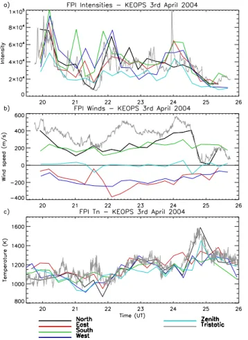
Fig. 2. FPI data from KEOPS on 3 April 2004 (a) intensities, (b) winds, and (c) temperatures.
10-s resolution data is 0.05 Hz. This results in over-sampling of the other look directions, but the important high resolution data is properly resolved.
The FPI data for the 3 April 2004 are shown in Fig. 2. The high time resolution of the tristatic data clearly shows much greater random variability than the other look direc-tions. This is especially true for the intensities in Fig. 2a, which vary on shorter time scales than the winds and tem-peratures. Line-of-sight winds comprise of meridional, zonal and vertical components. The look direction for the tristatic position has an azimuth of 43◦, with a 45◦elevation angle. The tristatic winds in Fig. 2b follow the general pattern of the north winds, which are not geographically far from the tristatic position, but they show much more structure. All the temperatures match reasonably well on a large scale when the changes are slow, for instance between 22:00 and 24:00 UT in Fig. 2c. However, when there are jumps in the temper-atures, such as in the intervals 20:00–22:00 UT and 24:00– 25:00 UT, the low resolutions of the other look directions do not see much of the variability of the tristatic data.
To see the variability of this high-resolution data more clearly, Fig. 3 zooms in on an hour section of the data from
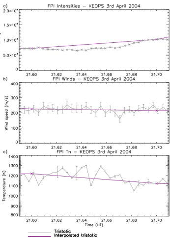
Fig. 3. 1 h of high resolution FPI data from KEOPS on 3 April 2004, including 0.1 h (6 min) interpolated tristatic data: (a) intensities, (b) winds, and (c) temperatures.
21:00–22:00 UT on Fig. 2. Only the tristatic and north look directions are shown for clarity. Error bars are shown for the winds and temperatures, but are not available for the un-calibrated intensities. The size of the temperature error de-terminations can vary wildly due to the analysis process, as the results of the least squares fitting routine is dependant on the quality and clarity of the interference fringes for each ex-posure. The overlaid purple line is an interpolation of the data at 0.1-h (6 min) resolution. This is the approximate res-olution of the data when a normal cycle of measurements is made, and any one look direction is measured just once in a cycle of seven measurements and a calibration lamp expo-sure. This shows the information that is lost on reduction of the time resolution. For example, the peaks in the intensi-ties in Fig. 3a, at 21.05 UT and 21.15 UT, are completely missed out in the interpolated data. The three reversals in the gradient of the wind direction around 21.2 UT in Fig. 3b are also not seen, nor is the fast variability from 21.6 UT to 21.7 UT. This variability is partly due to the low intensities at this time, as can be seen by comparing the period with Fig. 2a, which consequently gives a poor signal to noise ra-tio. This is also apparent as the variability is mostly within
E. A. K. Ford et al.: High time resolution measuements of the thermosphere 1273
Fig. 4. 10 min of high resolution FPI data from KEOPS on 3 April 2004, including 0.1 h interpolated tristatic data (purple line): (a) intensities, (b) winds, and (c) temperatures.
the error bars shown. This is also true of the temperatures in Fig. 3c through much of this period.
To show that these deviations from the interpolated data are real and not just noise, Fig. 4 shows the data zoomed in once more to a 6-min period (0.1 h). For this plot, the north data has been removed, and the individual data points for the intensities have been marked with crosses for further clarity, error bars are shown for the winds and temperatures. All three plots show structure in the high-resolution data not seen in the interpolated data. However, there are more data points than are needed here as the lines produce relatively smooth curves, so most of the structure in these data could be seen with data approximately every 0.02 h, or data with 1 min resolution. This implies a limit to the scale on which the thermosphere can vary, of approximately 1 min. Figure 5 shows a similar plot but from 21.6 to 21.7 UT. This is shown as this is during a period of low 630.0 nm emissions, and so shows the limit for a low signal to noise ratio period. The intensities show a similar response, with a similar difference in the detail between the high resolution data (gray) and the interpolated data (purple). For the temperatures and in par-ticular the winds, however, the signal is too low to provide
Fig. 5. 10 min of high resolution FPI data from KEOPS on 3 April 2004 from a low SNR period, including 0.1hr interpolated tristatic data (purple line): (a) intensities, (b) winds, and (c) temperatures.
as accurate results, and noise variations are seen at this scale. During the period with good signal to noise ratio (in Fig. 4), the 630.0 nm intensities have small noise levels. This is be-low the determined 1-min variability of the thermosphere, and so does not change this result for the intensities. The scale on which the thermosphere can vary, of approximately 1 min, is an important result as it is much shorter than the scale of 1 h on which the thermosphere is usually assumed to vary.
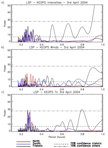
To determine the scale of the periodic variability in these data (as opposed to the random variability caused by, for ex-ample, auroral arcs), Lomb-Scargle periodograms are calcu-lated. The Lomb-Scargle periodogram of the above data is shown in Fig. 6. The spectral power is dependent on the time between data points, so the power is much larger for the tristatic data than the other look directions. Therefore, the other directions have been multiplied by a factor of ten so that all the directions can be seen on the same plot. The 70% confidence level for the tristatic data is shown with a dashed line. As the confidence levels are dependant on the time resolution of the data as well as the length of the night, a separate confidence level has been calculated for these other
Fig. 6. Lomb-Scargle Periodogram of FPI data from KEOPS on 3 April 2004: (a) intensities, (b) winds, and (c) temperatures. The low resolution look directions are scaled by a factor of ten for com-parisons.
directions. The 70% level for these is shown with a dot-dot-dash line. Note that the look directions are not in the same colours as Figs. 2 and 3 due to the different look directions plotted.
It should also be noted that, as the sampling interval of the periodogram is defined by the resolution of the tristatic A data, this results in the other directions being oversampled, and so periods less than the resolution of the data are tested for. All the peaks under the Nyquist frequency are well below the 70% confidence level (dot-dot-dashed line) and is there-fore within the noise and an artefact of the sampling. This is an additional reason why peaks with a confidence level this low are not considered real. However, for the tristatic data, the peaks at these short periods are above the 70% confidence level (the dashed line for tristatic data), and so are real wave peaks and not just the noise, as is the case with the other directions.
The relative amplitudes of the oscillations in the tristatic direction data appear larger than for any of the other direc-tions. This is an artefact of the temporal sampling and the Lomb-Scargle analysis, as spectral power is dependent on
the sampling frequency of the data, which was greater for the tristatic data. Plots of period, or frequency, against am-plitude of the wave would remove this difference, however it is of importance here to know if the waves observed are significant or not, and hence the spectral power is used.
All the parameters show several periodicities over through the whole range of periods within the measured boundaries, i.e., from half the length of the night down to the Brunt-V¨ais¨al¨a frequency (0.2 h period). Not all periods appear in all three parameters. It would not be necessarily expected that the winds should show similar periods to the other parame-ters, as gravity waves in the winds are affected by feedback mechanisms from the background wind field. The 630.0 nm intensities and the temperatures would be more likely to show the same periodicities as they are both affected by the energy input to the atom. There is a strong wave of 2-h period (±0.1 h) in all the parameters in the high-resolution tristatic data. There appears to be a wave at 1.5 h in all parameters, though for the winds, the power blends with the 2-h wave. There are also periods around 1 h, and several at shorter pe-riods.
To see these short period waves more clearly, periods up to 1 h are re-plotted on a different scale in Fig. 7. For this plot, the low time resolution data (i.e. all but the tristatic data) have been scaled by a factor of 4. Many peaks above the 70% confidence level (and in fact over the 99% confidence level, though this is not shown for clarity of the plot) can be seen at several periods down to 0.23 h (13.8 min) in the intensities, 0.26 h (15.6 min) in the winds and 0.27 h (16.2 min) in the temperatures. Uncertainties for these high-resolution data are approximately ±0.01 h, which is roughly twice the time resolution of the data. Few of the peaks in the other look di-rections reach the 70% confidence level, due to the poor sam-pling of the wave with the time resolution available. Only a selection of the look directions are shown in these plots, for clarity. Few of the periods seen in the tristatic data are seen at lower powers in the other directions, which corroborates the importance of high time resolution measurements in de-tecting short period waves.
Many other periods are seen from these periods up to an hour, some of them are seen in more than one parameter, but several are only seen in one parameter. To better compare the three parameters, the tristatic periodograms are plotted on the same graph in Fig. 8. Intensities are shown in red, winds in green, and temperatures in blue. A running smooth value of 120 points was removed from these data, which corresponds to approximately 30 min with this high time resolution data. This value is used as it removes the larger trends, and so re-moves power from the longest periods, those not associated with gravity waves, but is not so small as to remove power from the periods of interest. There are two main sources of longer scale periodicity: the diurnal maxima and minima in the temperatures due to dayside solar heating, and at high-latitudes, the two-cell ionospheric convection pattern drives the neutral winds via ion drag.
E. A. K. Ford et al.: High time resolution measuements of the thermosphere 1275
Fig. 7. Lomb-Scargle Periodogram up to periods of 1 h, from KEOPS data on 3 April 2004: (a) intensities, (b) winds, and (c) temperatures. The low resolution look directions are scaled by a factor of 4.
Fig. 8. Lomb-Scargle Periodogram of smoothed intensities, winds, and temperatures, from KEOPS data on 3 April 2004, using a 30-min running smoothing value.
Fig. 9. Lomb-Scargle Periodogram up to periods of 1 h, from KEOPS data on 5 April 2004: (a) intensities, (b) winds, and (c) temperatures. The low resolution look directions are scaled by a factor of 4.
Several periods have high spectral powers in two of the three parameters, such as at 0.46, 0.50, 0.66 and 1.0 h. How-ever, there are few periods where the peak is above the 70% confidence level in all three parameters. The only instance of this in this data set is at 0.32 h (19.2 min). As this is the only occurrence out of several peaks, this is possibly just a coincidence, rather than a mechanism that drives all three parameters in the same way. From the results from the sec-ond tristatic campaign (shown in Ford et al., 2006), it would be expected that the intensities and temperatures would pro-duce peak powers at the same periods. The winds would not necessarily show these same periods however, due to the winds having a more complicated relationship with the grav-ity wave parameters, for example because there is a feedback between the velocity of the wave and the velocity of the back-ground wind field. However, this effect is not clearly seen in Fig. 8, as the periods that are seen in two of the parameters are not always the same pair, and are various combinations of the three parameters.
Fig. 10. Lomb-Scargle Periodogram up to periods of 1 h, from KEOPS data on 10 April 2004: (a) intensities, (b) winds, and (c) temperatures. The low resolution look directions are scaled by a factor of 4.
Lomb-Scargle periodograms from the other clear nights during this experiment are shown in Figs. 9, 10, and 11, from 5, 10 and 11 April 2004, respectively. Periods up to 1 h are shown, and all the nights show several peaks with periods less than 1 h. On 5 April 2004, the intensities show a peak at 0.29 h in the tristatic data, above the 99% confidence level, that is also seen in the north intensities. Although this period is also seen in the winds and temperatures on this night: in the south, east, west, and zenith directions in the winds, and in all look directions for the temperatures, it is mostly not above the 70% confidence level, which highlights the impor-tance of high resolution data in detecting the waves with real certainty. Amongst the other peaks throughout the data, pe-riods of 0.48 and 0.57 h are present in all three parameters.
The 10 April 2004 data in Fig. 10 again show many short period gravity waves. The winds and temperatures however show slightly less waves than other nights at high confidence levels. For instance, there are only two peaks in the temper-atures above the 70% confidence level, in the south tion. There are peaks in the intensities in all the look
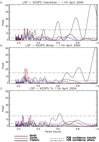
direc-Fig. 11. Lomb-Scargle Periodogram up to periods of 1 h, from KEOPS data on 11 April 2004: (a) intensities, (b) winds, and (c) temperatures. The low resolution look directions are scaled by a factor of 4.
tions at 2.3, 2.5, and 2.9 h, though again only above the 70% level in the high time resolution tristatic data. Several peri-ods are also seen in the data of 11 April 2004 in Fig. 11, but again there is little correlation between the three parameters for most of these short period waves.
4 Conclusions
Results from a high time resolution study of FPI data of the upper thermosphere in April 2004 allowed the variability of the thermosphere to be determined. The tristatic position was viewed at approximately 15-s resolution, made possi-ble by a new EMCCD camera. In addition, a full cycle of measurements were taken only every 16 min, so the effect of slow mirror rotation time was removed from the data. On in-spection of any random 10 min period of the high-resolution data from KEOPS, features in the data can be seen to con-tain many data points. These structures seen in the high-resolution data were compared with interpolated. This im-plies a limit to the scale on which the thermosphere can vary,
E. A. K. Ford et al.: High time resolution measuements of the thermosphere 1277 as more detail is not obtained when higher time resolutions
were used. From the data viewed here, this limit appears to be approximately one minute. This shows that the thermo-sphere can vary on scales down to one minute, not just the often-assumed value of approximately one hour.
Small scale periodic variability has also been detected in these thermospheric data. The four nights of high resolution data show that short period gravity waves are often seen in the FPI data from the high-latitude thermosphere. Waves are seen down to the order of the Brunt-V¨ais¨al¨a frequency, the limiting frequency at which waves can be sustained. These short period waves are not often seen with any confidence in the look directions with poor (16 min) time resolutions. This highlights the need for high time resolution data, and hence good detector technology, for the detection of short period gravity waves. On 3 April 2004, periods down to 14 min were seen in the 630.0 nm intensities, with similar periods in the winds and temperatures. Gravity waves with these short periods were seen on several nights, and on all of the three other clear nights when this high-resolution experiment was performed. This implies that short period gravity waves are present reasonably often, and the nights shown are not un-representative of the typical state of the thermosphere. This also supports the findings of the high level of variability and small scale structure that is present in the high latitude ther-mosphere.
Acknowledgements. The FPIs were built and maintained with
thanks to PPARC grant PPA/G/O/2001/00484. We also wish to ac-knowledge the ESRANGE KEOPS facility for their generous help in logistics. The MIRACLE network, which runs the Muonio All Sky Camera, is operated as an international collaboration under the leadership of the Finnish Meteorological Institute.
Topcial Editor U.-P. Hoppe thanks J. Lilensten and M. Conde for their help in evaluating this paper.
References
Aruliah, A. L., Fuller-Rowell, T. J., and Rees, D.: The Combined Effect of Solar and Geomagnetic Activity on High-Latitude Thermospheric Neutral Winds: I: Observations, J. Atmos. Terr. Phys., 53, 467–483, 1991.
Aruliah, A. L. and Griffin, E. M.: Evidence of meso-scale structure in the high latitude thermosphere, Ann. Geophys., 19, 37–46, 2001,
http://www.ann-geophys.net/19/37/2001/.
Aruliah, A. L. and Rees, D.: The trouble with thermospheric verti-cal winds: geomagnetic, seasonal and solar cycle dependence at high latitudes, J. Atmos. Terr. Phys., 57, 597–609, 1995. Aruliah, A. L., Griffin, E. M., Aylward, A. D., Ford, E. A. K.,
Kosch, M. J., Davis, C. J., Howells, V. S. C., Pryce, E., Middle-ton, H., and Jussila, J.: First direct evidence of meso-scale vari-ability on ion-neutral dynamics co-located tristatic FPIs and EIS-CAT radar in Northern Scandinavia, Ann. Geophys., 23, 147– 162, 2005,
http://www.ann-geophys.net/23/147/2005/.
Aruliah, A. L., Griffin, E. M., McWhirter, I., Aylward, A. D., Ford, E. A. K., Charalambous, A., Kosch, M. J., Davis, C. J., and How-ells, V. S. C.: First tristatic studies of meso-scale ion-neutral dy-namics and energetics in the high-latitude upper atmosphere us-ing collocated FPIs and EISCAT radar, Geophys. Res. Lett., 31, L03802, doi:10.1029/2003GL018469, 2004.
Balthazor, R. L. and Moffett, R. J.: Morphology of large-scale travelling atmospheric disturbances in the polar thermosphere, J. Geophys. Res., 104, 15–24, 1999.
Brekke, A.: Physics of the Upper Polar Atmosphere, Wiley, Chich-ester, 1997.
Burnside, R. G. and Tepley, C. A.: Optical Observations of Ther-mospheric Neutral Winds at Arecibo between 1980 and 1987, J. Geophys. Res., 94, 711–716, 1989.
Codrescu, M. V., Fuller-Rowell, T. J., Foster, J. C., Holt, J. M., and Cariglia, S. J.: Electric field variability associated with the Millstone Hill electric field model, J. Geophys. Res., 103, 5265– 5273, 2000.
de Deuge, M. A., Greet, P. A., and Jacka, F.: Optical observations of gravity waves in the auroral zone, J. Atmos. Terr. Phys., 56, 617–629, 1994.
Ford, E. A. K., Aruliah, A. L., Griffin, E. M., and McWhirter, I.: Thermospheric gravity waves in Fabry-Perot Interferometer measurements of the 630.0 nm OI line, Ann. Geophys., 24, 555– 566, 2006,
http://www.ann-geophys.net/24/555/2006/.
Hernandez, G. and Roble, R. G.: The Geomagnetic Quiet Night-time Thermospheric Wind Pattern Over Fritz Peak Observatory During Solar Cycle Minimum and Maximum, J. Geophys. Res., 89, 327–337, 1984.
Hocke, K. and Schlegel, K.: A review of atmospheric gravity waves and travelling ionospheric disturbances: 1982–1995, Ann. Geo-phys., 14, 917–940, 1996,
http://www.ann-geophys.net/14/917/1996/.
Hunsucker, R. D.: Atmospheric gravity waves generated in the high-latitude ionosphere: a review, Rev. Geophys. Space Phys., 20, 293–315, 1982.
Innis, J. L. and Conde, M.: High-latitude thermospheric verti-cal wind activity from Dynamics Explorer 2 Wind and Tem-perature Spectrometer observations: Indications of a source re-gion for polar cap gravity waves, J. Geophys. Res., 107, 1172, doi:10.1029/2001JA009130, 2002.
Innis, J. L. and Conde, M.: Thermospheric vertical wind activity maps derived from Dynamics Explorer-2 WATS observations, Geophys. Res. Lett., 28, 3847–3850, 2001.
Innis, J. L., Greet, P. A., and Dyson, P. L.: Thermospheric grav-ity waves in the southern polar cap from 5 years of photometric observations at Davis, Antarctica, J. Geophys. Res., 106, 15 489– 15 500, 2001.
Jerram, P., Pool, P., Bell, R., Burt, D., Bowring, S., Spencer, S., Hazelwood, M., Moody, I., Catlett, N., and Heyes, P.: The LLL-CCD: Low Light Imaging without the need for an intensifier, Proc. SPIE, 4306, 178–186, 2001.
Kivelson, M. G. and Russell, C. T.: Introduction to Space Physics, Cambridge, Cambridge University Press, 1989.
Lomb, N. R.: Least squares frequency analysis of unequally spaced data, Astrophys. Space Sci., 39, 447–462, 1976.
MacDougall, J. W., Andre, D. A., Sofko, G. J., Huang, C. S., and Koustov, A. V.: Travelling ionospheric disturbance properties
duced from Super Dual Auroral Radar measurements, Ann. Geo-phys., 18, 1550–1559, 2001,
http://www.ann-geophys.net/18/1550/2001/.
Niciejewski, R., Killeen, T. L., and Solomon, S. C.: Observations of thermospheric horizontal neutral winds at Watson Lake, Yukon Territory (Lambda=65 N), J. Geophys. Res., 101, 241–259, 1996. Rishbeth, H. and Garriott, O. K.: Introduction to Ionospheric
Physics, Academic Press, 1969.
Scargle, J. D.: Studies in Astronomical time series analysis: II Sta-tistical aspects of spectral analysis of unevenly spaced data, As-trophys. J., 263, 835–853, 1982.
Solomon, S. C., Hays, P. B., and Abreu, V. J.: The auroral 6300A emission: observations and modeling, J. Geophys. Res., 93, 9867–9882, 1988.
Wang, W., Killeen, T. L., Burns, A. G., and Roble, R. G.: A high-resolution, three-dimensional, time dependent, nested grid model of the coupled thermosphere-ionosphere, J. Atmos. Solar Terr. Phys., 61, 385–397, 1999.
Williams, P. J. S., Virdi, T. S., Lewis, R. V., Lester, M., Rodger, A. S., McCrea, I. W., and Freeman, K. S. C.: Worldwide atmo-spheric gravity-wave study in the European sector 1985–1990, J. Atmos. Terr. Phys., 55, 683–696, 1993.