Dijet production in polarized proton-proton collisions at [the square root of sigma] = 200 GeV

Dijet production in polarized proton-proton

collisions at

VI-s

OF TECH4NOLOGCrY

by

~~~ ~

~

OCT

3 12011

Matthew Walker

L iBR:,AR IE S

Submitted to the Department of Physics

in partial fulfillment of the requirements for the degree of

ARCHIVES

Doctor of Philosophy in Physics

at the

MASSACHUSETTS INSTITUTE OF TECHNOLOGY

June 2011

@Massachusetts

Institute of Technology 2011.

A u th o r

... ..

.

All rights reserved.

Department of Physics

April 29, 2011

Certified by

_{... ,..}

_{* j}

Bernd

Surrow

Associate Professor

Thesis Supervisor

Accepted by ...

_...

Krishna Rajagopal

Associate Department Head for Education

Dijet production in polarized proton-proton collisions at

s

= 200 GeV

by

Matthew Walker

Submitted to the Department of Physics on April 29, 2011, in partial fulfillment of the

requirements for the degree of Doctor of Philosophy in Physics

Abstract

Polarized deep inelastic scattering (DIS) experiments indicate that quarks only carry approximately 30% of the proton spin, which led to interest in measuring the con-tributions of other components. Through polarized proton-proton collisions at the Relativistic Heavy Ion Collider (RHIC), the world's only polarized proton collider, it is possible to make an extraction of the polarized gluon distribution function Ag(x). This function describes the contribution of the gluon polarization to the proton spin.

This thesis presents a measurement of the p + p ---> Jet + Jet + X (dijet) cross

section from the 2005 RHIC running period and a measurement of the longitudinal double spin asymmetry ALL from the 2009 RHIC running period, both made using the Solenoidal Tracker at RHIC (STAR). The cross section is measured over the invariant

mass range 20 < M < 116 GeV/c 2 _{with systematic uncertainties between 20 and}

50%, driven by the jet energy scale uncertainty. The asymmetry is measured over the

invariant mass range 20 < M < 80 GeV/c 2 in three different detector acceptances.

The asymmetry measurement is compared to several theory scenarios in each of the detector acceptances, which allows extraction of the shape of the polarized gluon distribution function Ag(x). The results are consistent with a small, but positive, total gluon polarization.

Thesis Supervisor: Bernd Surrow Title: Associate Professor

Acknowledgments

There are many people who I need to thank for helping make this thesis possible. First, my advisor, Bernd Surrow, whose passion for the RHIC-Spin program and dedication to producing important results allowed me to work on this exciting analysis and whose support helped me forge ahead. Bob Redwine provided important guidance in navigating the political waters of the STAR collaboration and in managing the thesis writing "problem."

I am in debt to many people who supported and scrutinized this analysis, the core of whom were past and present members of the RHIC-Spin group: Renee Fatemi, Ross Corliss, Fang Guo, James Hays-Wehle, Alan Hoffman, Chris Jones, Adam Kocoloski, William Leight and Tai Sakuma. Special mentions need to be made for Jan Balewski, whose enthusiasm led to my simulation being completed on the cloud, and for Joe Seele and Mike Betancourt, for many discussions about all aspects of the analysis and support in the face of adversity. Members of the STAR collaboration deserve my gratitude. Stephen Trentalange has been exceptionally supportive and taught me much about calorimeters. J6rume Lauret helped me explore cloud computing in physics and supported my efforts as part of the Software and Computing team.

Many people gave me opportunities to enjoy life outside of work, including the members of Statmechsocial, Physics GSC, Ultimate Pickup and the Sidney-Pacific community. Roger and Dottie Mark and Roland Tang and Annette Kim have kept me well fed over the past few years. Nan Gu pressed me to get involved in many extracurriculars. The Feng and Benz families have been enormously supportive. My brother, Nick, and sister, Liz, never failed to lift my spirits or to let me get complacent. My girlfriend has supported, entertained and commiserated with me even as she works on her own doctoral studies. Thank you for putting up with me, Annie.

Finally, I can hardly express the gratitude I have for my parents. From them, I have inherited my curiosity, pragmatism and perseverance. They have supported and prodded me through many challenges and have always looked out for my best interests. Mom, Dad, Thank you.

Contents

1 Introduction

1.1 Early Proton Structure . . . .

1.2 Deep Inelastic Scattering . . . .

1.3 Quantum Chromodynamics . . . .

2 Experimental Setup

2.1 RHIC ... ...

2.1.1 Polarized proton source . . .

2.1.2 Preinjection . . . .

2.1.3 Storage ring . . . .

2.1.4 Maintaining and Monitoring

2.2 STAR ... ... .. 2.2.1 BEMC . . . . 2.2.2 TPC . . . . 2.2.3 BBC . . . . 2.2.4 ZDC . . . .. . .. . . . . . Polarization

Different Levels of Jets .. . . . . Theoretical Background . . . . Jet Finding in STAR . . . . 4 Simulation 21 22 23 29 35 35 35 37 38 39 43 43 47 49 49 53 53 54 56 61 3 Jets 3.1 3.2 3.3

4.1 Event Generation . . . .

4.1.1 PYTHIA ...

4.1.2 Tuning PYTHIA .

4.2 STAR Simulation Framework

4.3 Simulation Productions . 4.3.1 2005 Simulation . 4.3.2 2009 Simulation . 5 Cross Section 5.1 _{D ata Set . . . .} 5.2 M easurem ent . . . .

5.2.1 Reconstructed Dijet Trigger Efficiency . . . .

5.2.2 Misreconstruction Efficiency . . . .

5.2.3 _{Unfolding Matrix . . . .}

5.2.4 Particle Dijet and Vertex Reconstruction Efficiency

5.2.5 _{Trigger Time Bin Acceptance Correction . . . .}

5.2.6 Integrated Luminosity . . . .

5.3 Dijet Statistical Uncertainties . . . . 5.4 Dijet Systematic Uncertainties . . . .

5.4.1 Normalization Uncertainty . . . .

5.4.2 Vertex Acceptance Uncertainty . . . .

5.4.3 Reconstructed Dijet Trigger Efficiency Uncertainty

5.4.4 _{Jet Energy Scale Uncertainty . . . .}

5.4.5 Beam Background Uncertainty . . . .

5.5 Theory Calculation . . . .

5.6 Hadronization and Underlying Event Correction . . . .

5.7 Results 6 Asymmetry 6.1 D ata Set . . . . 6.2 M easurem ent . . . . . . . . 6 1 . . . . 6 2 . . . . 6 2 . . . . 6 3 . . . . 6 5 . . . . 6 5 . . . . 6 5 67 . . . . 67 . . . . 67 . . . . 72 . . . . 76 . . . . 77 . . . . 79 . . . . 81 . . . . 82 . . . . 83 . . . . 84 . . . . 84 . . . . 84 . . . . 85 . . . . 86 . . . . 90 . . . . 91 . . . . 91 . . . . 9 5

6.3 6.4 6.5 6.6 6.2.1 Polarization . . . . . 6.2.2 Relative Luminosity 6.2.3 Unfolding Matrix Statistical Uncertainties Systematic Uncertainties Theory Calculation . . . . . Results . . . . 7 Conclusions

A Calibration of the BEMC

A.1 2006 M ethods . . . . A.2 2006 Uncertainty . . . . A.3 Updates to Methods in 2009 . . . .

A.3.1 PMT Mapping Check . . . .

A.3.2 HV adjustment . . . .

A.4 2009 Uncertainty . . . . A.5 Conclusions . . . . B BEMC Simulation Chain Model

C Cloud Computing for STAR Simulations

C.1 Virtualization . . . . C.2 Cloud Computing . . . .

C.3 Kestrel. .. ... .. .. . . . .. .

C.4 STAR Simulation on the Cloud...

D Logical Deduction of Cross Section Formula E Tests of the Unfolding Method

E.1 Comparison of Matrix Unfolding with Bin-by-bin . . . . 9 101 103 110 111 113 115 115 123 125 125 128 135 137 138 139 141 143 147 147 149 149 150 155 157 159 . . . . . . . . . . . . . . . .

F Spin-Sorted Yields in Simulation ₁₆₁

F.1 Sim ple Derivation ... . 161

F.2 Probabilistic Derivation ... ... 162

F.3 A pplication . . . 163

F.4 Comparison to Method of Asymmetry Weights . . . 164

List of Figures

1-1 The particles arranged in the meson octet in the Eightfold Way have

horizontal lines of constant strangeness and diagonal lines of constant

electric charge . . . . 22

1-2 A simple Feynman diagram illustrating deep inelastic scattering (DIS),

in which an electron scatters off a quark in the target proton. .... 24

1-3 Measurements of the first moment of gi(x) by the EMC experiment

are shown by the left axis and the crosses. The data disagree with the

Ellis-Jaffe calculation (shown top left) [1]. . . . . 28

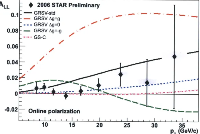
1-4 An early measurement of ALL using inclusive jets from STAR in 2006

constrained AG, in particular excluding large positive values. ... 31

1-5 STAR data contributed to a significant constraint on a global

extrac-tion of A

g(x)

[2]. . . . .

32

1-6 This Feynman diagram depicts the collision of two protons, pi and

P2. The colliding quarks, x1 and x2, have momentum fraction x of

their respective protons. Outgoing quarks, P3 and p4, can be used to

calculated the initial quark kinematics. . . . . 32

1-7 A leading-order diagram in QCD for quark-gluon scattering. ... 33

2-1 A schematic of RHIC's polarized proton source. Protons from the ECR source enter at the left and polarized H- exits at 35 keV from the lower

right [3] . . . . 36

2-2 A diagram labeling the different sections of the AGS to RHIC transfer

2-3 The precession of the spin vector for a transversely polarized beam as it traverses a full Siberian Snake along the beam direction (shown in

b lu e) . . . . 4 0

2-4 A diagram of the H-Jet polarimeter . . . . 42

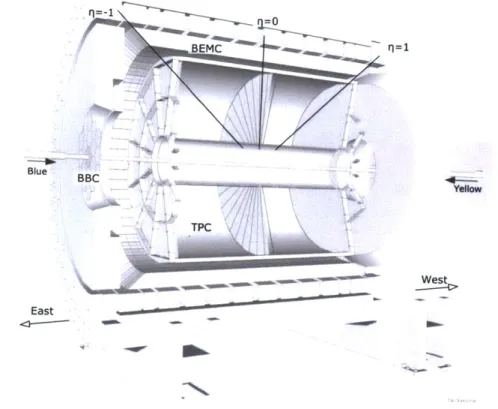
2-5 A diagram of the STAR detector with the primary detectors used for

the jet analysis labeled. . . . . 44

2-6 A cross section of a BEMC module showing the mechanical assembly of a tower including the compression components and the location of

the shower maximum detector. . . . . 45

2-7 The STAR TPC provides large acceptance tracking of charged

parti-cles, vertex reconstruction, and particle identification. . . . . 48

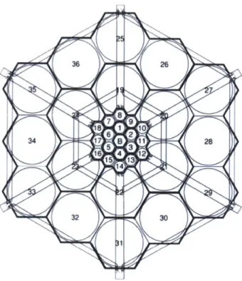
2-8 The STAR BBC. The inner 18 tiles are used for this analysis. The "B"

represents the beam pipe. . . . . 50

2-9 The ZDC is positioned past the DX bending magnets so that only

neutral particles enter it. . . . . 51

3-1 An event display of a dijet event taken during Run 9, displaying tracks

reconstructed in the TPC and energy depositions measured in the BEMC. 56

4-1 The STAR simulation framework with the locations in which filters can be inserted. Steps 1, 2, and 3 are implemented in STARSIM using

StMcFilter and step 4 is implemented in BFC using StFilterMaker. . 65

5-1 The trigger turn-on for the BJP2 trigger as a function of reconstructed Jet Patch ET. The plateau value is at 0.95. This analysis used a cut

at 8.5 GeV to be above the turn-on. . . . . 69

5-2 The trigger turn-on for each jet patch for BJP2. The threshold varied from patch to patch due to the difference between the ideal calibration used for the trigger threshold and the actual calibration calculated later. 70

5-3 The raw yields from the simulation sample after passing all of the same cuts as the data raw yields. The events were reweighted based on their vertex to match the data vertex distribution. The events from different

partonic PT bins were added using the cross section weights, so these

yields are scaled by those weights. . . . . 73

5-4 The figure shows the comparison of reconstructed dijet distributions in data and simulation after all the same cuts are applied. Data are red

in the figures and simulations are blue. . . . . 74

5-5 The vertex distribution for dijet events in data (within time bins 7 and 8) varies from the distribution for simulation, so a reweighting was

applied based on the ratio of the distributions. . . . . 75

5-6 The relation between Mreco and Mparticie was used to determine the

un-folding matrix. This histogram shows the unnormalized contributions of each bin in detector invariant mass to each bin in particle invariant

m ass. . . . . 79

5-7 The BBC time bin distribution for the minimum bias trigger. .... 82

5-8 The BBC time bin distributions for the minimum bias trigger (black) and the BJP2 trigger (red) were noticeably different. The BJP2

dis-tribution has been rescaled for comparison. . . . . 85

5-9 A graphic showing where the two BEMC energy scales, the ExBES and the McBES, were used in calculation involving simulated data or

real data. ... ... 87

5-10 The black curve on this figure displays the raw data dijet yields. The red curves were produced by recalculating the yields using calibration tables that were shifted high and low. The blue curves were produced

5-11 The 2005 Dijet Cross Section. The uncertainty bars represent the statistical uncertainties on the measurement including the uncertainties due to the finite statistics in the Monte Carlo sample. The yellow bands carry the uncertainties in the jet energy scale. The top plot shows the value of the cross section and the bottom plot shows the comparison

to theory. ... ... 96

5-12 A comparison between theory and data for different cone radiuses with the hadronization and underlying event correction included shows sig-nificant cone radius dependence. This comparison was calculated using

2006 data in another analysis [4]. . . . . 97

6-1 Agreement between the data and simulation for the 2009 analysis is

good... ... 102

6-2 The difference in the data/simulation agreement between high and low

luminosity data confirms that the small discrepancy in the q34

distri-bution was caused by pileup tracks, which entered more as luminosity

increases. ... ... 102

6-3 The polarizations for the blue and yellow beams as a function of fill

with statistical uncertainties included. . . . 104 6-4 The ratio of the ZDC coincidence rate to the BBC coincidence rate

before any corrections were applied as a function of bunch crossing. . 106

6-5 The ratio of the ZDC coincidence rate to the BBC coincidence rate after being corrected for the singles and multiples rates as a function of bunch crossing. . . . 107

6-6 The difference between the R3 values calculated using the BBC

coin-cidence scaler and the ZDC East scaler shows very good agreement. . 109

6-7 The so-called false asymmetries were consistent with zero, which im-proved confidence that there was no spin dependent effect in the trig-gering and relative luminosity calculations. . . . 116

6-8 The false asymmetries remained consistent with zero, perhaps even improving consistency, after unfolding, which improved confidence that

the procedure did not bias the asymmetry calculation. . . . . 117

6-9 Comparisons of the unpolarized unfolding with the polarized unfolding

for different theory scenarios were used to calculate an uncertainty for visual comparison between the asymmetry and multiple theory curves. 118

6-10 The final longitudinal double spin asymmetry with comparisons to var-ious theory scenarios including statistical and systematic uncertainties. The difference panels are the different acceptances: same side jets on the left, opposites side jets in the middle, and the full acceptance on

the right . . . . 121

6-11 The leading order sensitivity to the parton kinematics (in the form of Bjorken-x) is different for the various mid-rapidity acceptances, which allows constraints to be placed on the shape of Ag(x). The left two panels show distributions for dijets with both jets on the east side of the BEMC and the right two panels show distributions for one jet on each

side of the BEMC. The top panels show the x1 and X2 distributions for

two mass bins and the the bottom panels show the mean and RMS of

the x1 and X2 distributions for each bin. . . . . 122

A-1 The MIP peak for each tower was fit with a gaussian (in blue) and the value of the peak position was used to provide the relative calibration

between towers. . . . . 126

A-2 The electron E/p spectrum for one of the rings showing the correction applied for that ring to the absolute energy scale. This figure has

A-3 This plot of track momentum p vs. E/p for electrons from HT/TP events shows that there was a clear momentum dependence of E/p for these electrons. Notice the curve in the spectrum and that it began before the area where the momentum reach of the non-HT/TP events falls off. That dependence had disappeared when we look at electrons for non-HT/TP events. Even though the momentum reach was re-duced, the curve had clearly disappeared. These plots only used the restricted data sample. . . . 129 A-4 Four different cut scenarios were looked at after all stringent cuts were

applied to determine the systematic uncertainty due to the trigger bias. The y-axis of this plot is E/p and the points represent one of the sce-narios. Scenario 1 was all of the electrons after stringent cuts. Scenario 2 was electrons from events that were non-HT/TP triggered. Scenario 3 was electrons from events that were HT/TP triggered. Scenario 4 was electrons from HT/TP events with tracks from the trigger turn-on

region (4.5 < p < 6.5 GeV/c) removed. The largest difference from

here, which corresponded to Scenario 3 defined the uncertainty from

the trigger bias at 1.3% . . . . 130

A-5 The non-HT/TP triggered events demonstrate linearity in the detector

over the electron momentum range 2 - 5 GeV/c as shown in this plot

of E/p vs. momentum. . . . . 131

A-6 As the lower cut on dE/dx was raised (removing more background), we see that the Gaussian + Line model had better stability than just a Gaussian. The lower cut on dE/dx of 3.5 keV/cm used for this study

coincides with where the E/p location plateaus for both models. . . . 132

A-7 Excluding Crate 12, there was no deviation beyond the expected sta-tistical in the scatter of E/p for each crate. The axis here starts from 0 instead of 1. This figure only contains electrons from the restricted

A-8 A comparison between the RMS for different numbers of divisions in pseudo-rapidity and when an additional 1% systematic was introduced shows that there was no pseudo-rapidity dependent systematic

uncer-tainty. This figure only contains electrons from the restricted sample. 134

A-9 E/p vs ZDC rate was calculated for the tightened calibration sample. The three points show the E/p peak location for different ranges of ZDC rate, which were chosen to have roughly equal statistics. Point

1 corresponds to 0 - 8000 Hz, 2 corresponds to 8000-10000 Hz and 3

corresponds to 10000-20000 Hz. . . . . 134

A-10 The entire 2006 calibration electron sample was used to examine the time dependence. The first period was for before day 110. The second period was for between days 110 and 130. The third period was after

day 130. . . . . 135

A-11 The distribution of E/p corrections in a given pseudorapidity ring did

not have statistical variation, as demonstrated by this plot of X2/NDF

for the distribution of E/p in each ring. . . . . 136

A-12 The GEANT correction for each pseudorapidity ring. This correction multiplies the track momentum of the calibration electron depending

on the distance it strikes the tower from its center. . . . . 137

A-13 A comparison of the distribution of full scale ET for all calibrated

towers for run 9 (top) and run 8 (bottom). The left panels show the distributions for all towers, the center panels show the distributions for the towers with |g| < 0.9, and the right panels show the distributions for the towers with 11 > 0.9. . . . 139 A-14 This figure shows the overall E/p peak location for each run before the

calibration is applied as a function of an arbitrary, time-ordered run

index. The slope of the best fit is non-zero, but extremely small. . . . 140

A-15 E/p as a function of R = /(A#) 2 _{+ (Aj)2. The shape of the figure}

resembles a sinusoid, but there was no obvious physical reason why

B-1 A model of the BEMC detector simulation chain. It tracks the simula-tion from the intitial generated physics event, through its interacsimula-tion with the detector, the characterization of the active elements in the slow simulator and then finally through our calibrations and energy scales to the final reconstructed energy. . . . 144 C-1 A diagram depicting how virtual machine monitors interact with

hard-ware, operating systems, and applications in system virtual machines. 148

C-2 Tracking the number of jobs as a function of time in the PBS and Kestrel systems. The number of virtual machines instantiated tracks the number of available nodes, indicating a good response of the sys-tem. A guaranteed allocation of 1,000 slots for a few days around July 21 shows we exceeded the allocation and took advantaged of empty slots on the farm . . . 152

E-1 An unfolding matrix was caluclated for an input distribution of f (x) =

1

T and a gaussian point spread function with o = 1. This figure shows

the unfolding performance for unknown input distributions of the form

f (x ) = x" . . . . . . . . . . . . . . . . . . . . . . . . . . . . . . . . . 158

E-2 (Top panel)A comparison of the cross section using the matrix unfold-ing (black) with the bin by bin unfoldunfold-ing (red) and statistical uncer-tainties only. The most important difference is the inability of the bin by bin method to extract the cross section in the last bin. (Bottom panel) The ratio of bin by bin cross section over the matrix cross sec-tion with statistical uncertainties only. The different methods do not

List of Tables

3.1 Example PYTHIA Record. . . . . 58

4.1 2005 Dijet Simulation Productions . . . . 66

4.2 2009 Dijet Simulation Productions . . . . 66

5.1 Raw Dijet Yields . . . .. 72

5.2 Trigger Efficiency . . . . 76

5.3 Misreconstruction Efficiency . . . . 77

5.4 Unfolding M atrix . . . . 80

5.5 Vertex and Reconstruction Efficiency . . . . 81

5.6 Expected statistical uncertainties compared with actual statistical un-certainties . . . . 84

5.7 Energy Uncertainty Contributions . . . . 90

5.8 Beam Background Uncertainty . . . . 90

5.9 Hadronization and Underlying Event Simulations . . . . 93

5.10 Particle Reconstruction Efficiency for Hadronization/UE Correction . 93 5.11 Reconstruction Efficiency for Hadronization/UE Correction . . . . 93

5.12 Transfer Matrix for Hadronization/UE Correction . . . . 94

5.13 Data points and Uncertainties . . . . 95

6.1 Raw Dijet Yields for full acceptance analysis . . . . 101

6.2 Run 9 200 GeV Polarizations and Uncertainties . . . . 103

6.3 Relative Luminosity Definitions . . . . 105

6.5 6.6 6.7 6.8 6.9 6.10

Bunch Crossings Removed from Analysis Misreconstruction Efficiency . . . . Unfolding Matrix . . . . Reconstruction Efficiency . . . .

Description of False Asymmetries . . . .

Systematic Uncertainty Contributions . .

A.1 2006 Contributions to Uncertainty . . . . A.2 2009 Contributions to Uncertainty . . . . E.1 Unfolding Toy Model Performance . . . . E.2 Comparison of uncertainties for Bin by Bin versus

. . . . Matrix Unfolding . 108 111 112 113 114 119 141 142 159 159

Chapter 1

Introduction

The proton is a composite particle made up of quarks and gluons whose interactions are described by quantum chromodynamics (QCD). The spin structure of the proton remains an area of intense study by both experimentalists and theorists. It can be described in a simple picture as

1 1

-AE + Lq+AG+Lg _(1.1)

2 2

where AE represents the quark spin contribution, AG represents the gluon spin con-tribution, and Lq(g) represents the quark (gluon) orbital angular momentum. This relation can actually be constructed in QCD in the infinite momentum frame and the

light cone gauge [5].

Chapter 1 discusses the theoretical background of understanding the proton spin, taking a historical approach.

Chapter 2 describes the experimental setup of the Relativistic Heavy Ion Collider (RHIC) and the Solenoidal Tracker at RHIC (STAR), which were used to measure the gluon polarization in proton-proton collisions.

Chapter 3 covers the theoretical basis of jets and discuss methods for finding jets with a focus on the methods used in this thesis.

Chapter 4 describes the simulation package used to help understand physics and detector effects that need to be corrected for in the measurement of jet observables

s1 K= s=0 -+ 17 S q1 s =-1 K- K q= -1 q = 0

Figure 1-1: The particles arranged in the meson octet in the Eightfold Way have

horizontal lines of constant strangeness and diagonal lines of constant electric charge

and methods used to improve the quality of those simulations.

Chapter 5 explains the measurement of the dijet cross section in the RHIC run 5 data collected at STAR.

Chapter 6 explains the measurement of the dijet longitudinal double-spin asym-metry in the RHIC run 9 data collected at STAR.

Chapter 7 discusses the impact of these measurements and what future work can be done to expand on their results.

1.1

Early Proton Structure

Discovery of the proton can be attributed to Rutherford

[6],

nitrogen nuclei contained hydrogen nuclei. It was already known that the masses of the other nuclei were multiples of the mass of the hydrogen nuclei. Rutherford thus concluded that the hydrogen nucleus was a building block of the heavier nuclei and coined the term proton.

Hints that the proton had complicated internal structure included measurement of

its anomalous magnet moment

[7],

the Eightfold Way to explain the growing numbers of hadrons being discovered in cos-mic ray measurements and early accelerator experiments that there was a consistent way to describe that structure. Using charge and strangeness, Gell-Mann classified

the hadrons into a variety of multiplets based on their spin. The Quark Model, intro-duced by Gell-Man and Zweig in 1964, explained why the hadrons fit into categories so nicely by proposing that the hadrons were composite particles made of even smaller quarks.

The final touch to the quark model was the proposal that the quarks also carried a new kind of charge dubbed color by Greenberg [8]. This addition saved the quark model from conflict with the Pauli exclusion principle. The problem was caused by the A++, which the quark model suggested was made up of three up quarks in the same state. By introducing color, Greenberg was able to defuse the problem and save the quark model. To explain why only certain combinations of quarks are found in nature, the theory also requires that only colorless particles are stable.

The quark model provides a simple explanation of all of the baryon spins. Three spin 1 particles combine into two possible spin states,

1 1 1 3 1

- - @ - =- (D -.

2 2 2 2 2

Baryons with spin

j

of quark generation of baryon spin. Thus, the origin of the proton's spin has a straightforward explanation in a static model of the proton structure.

1.2

Deep Inelastic Scattering

While the quark model successfully explained the hadron hierarchy, observation of iso-lated free quarks was impossible under its rules. However, experiments using charged lepton beams on proton targets in deep inelastic scattering (DIS) finally gave access to the proton structure. Figure 1-2 illustrates the DIS process. The idea behind using electrons to probe the structure is that the scattering cross section is proportional to the squared form factor F(q) of a charge distribution [9]. The cross section can be written as

du

f

L~

dQ dQ point

Figure 1-2: A simple Feynman diagram illustrating deep inelastic scattering (DIS), in which an electron scatters off a quark in the target proton.

where F(q) is the Fourier transform of the charge distribution.

The situation becomes slightly more complicated for protons. The cross section for DIS can be described as

1

doc c LMW , _(1.3)

where LW" is the lepton tensor, which describes the physics on the lepton side of the photon propagator, and W,, is the hadronic tensor, which contains all of the information on the hadronic side.

In DIS, there are two Lorentz invariant quantities that describe the kinematics:

Q2

Q2 2p - q

where q is the momentum transfer through the photon and p is the proton momentum. The variable x is called Bjorken-x and is often interpreted in the infinite momentum frame as the fraction of the proton momentum carried by the struck quark.

Using charge conservation and the fact that the lepton tensor L" is symmetric,

it's possible to write the hadronic tensor in terms of two structure functions W1(Q2, X)

and W₂(Q2, x). The cross section becomes

da

, oc 4 (2Wi(Q2 , x) sin - W 2(Q2, X) cos2 _), (1.4)

dgdE

Q

electron.

Bjorken proposed that these functions are independent of Q2 _{in the deep inelastic}

scattering regime, which is a consequence of the point like nature of the proton con-stituents. This behavior is called Bjorken scaling and was confirmed by experiments at SLAC [10]. In this regime, the structure functions are rewritten as

MWI(Q2_{, x) -- + F1(x)}

Q2M W2(Q2, X) - F2(x).

2Mc2X

Callan and Gross went on to suggest that the two scaling functions are related by

2xF1(x) = F2(x), which was also confimed at SLAC.

In the parton model, the function F1(x) can be written as

F1(x) = IEZefi(X), (1.5)

i

where qj is the charge of a quark, fi(x) is the individual quark distribution function, and the sum over i is over both quark and anti-quark flavors. The quark distribution functions can be thought of as probability distributions for the amount of the proton's momentum carried by quarks of a certain flavor.

The proton includes not only the two up and one down valence quarks that pri-marily govern its characteristics, but also a sea of quarks and gluons that mediate the strong interaction. Therefore, the proton structure function should be

2F1(x) = ()2[U(X) +(X)] + (1)2[d(x) + d(z) + s(x) + s(x)], (1.6)

33

including the contributions of strange quarks, but not heavier quarks. The up quark distribution should have some contribution from the valence up quarks and some from the sea up quarks and the same for down quarks. We also expect all of the sea quarks

and anti-quarks should have approximately the same distributions:

u(x) = Uvaience(X) + Usea(X)

d(x) dvaience(X)+ dsea(x)

Usea(x) dsea(X) = U(x) = d(x) = s(x) = S(X).

Adding in the constraint that the quantum numbers of the proton must be conserved provide sum rules for the quark distribution functions:

[u(x) - i(x)]dx = 2,

f [d(x) - d(x)]dx = 1,

[s(x) - §(x)]dx = 0.

These sum rules, represented by the integrals over x, are actually sums over all quarks of the relevant flavor. The idea of a sum rule will be important below.

Using these quark distributions, it is possible to calculate the momentum fraction

carried by all quarks, eq:

e = jx qi(x)dx = 1 - eg, (1.7)

where qi(x) are again the quark distribution functions and e9 is the momentum

frac-tion carried by gluons. Experimental measurements of F2(x) for both the proton and

the neutron have found that eL = 0.36 and d = 0.18. By neglecting the contribution

from heavier quarks, that implies Eg = 0.46. So here is the first clear evidence that

the effects of the gluon are important in understanding the proton.

The same framework of quark distribution functions can be used to discuss the spin component of the proton. The polarized quark distribution functions Aq(x) are defined as [11]

where qi is the quark distribution function for quarks that are polarized along the direction of the proton's polarization and q is the quark distribution function for quarks with the opposite polarization. A quark spin-dependent structure function

g1(x) is defined in terms of these distribution functions as

gi(z) = : eAqi(x). (1.9)

i

Ellis and Jaffe derived a sum rule for gi(x) by assuming an unpolarized quark sea [12] for polarized DIS on both proton and neutron targets:

dxgp() = 1.78 (1.10)

jdxg["(x) -0.22 A (1.11)

12

where gA is the axial vector coupling. Experimental values of gA = 1.248 ± 0.010

correspond to

fji

Polarized DIS is sensitive to gi(x) by measuring two asymmetries [11]. Ali is the asymmetry for when the lepton and nucleon spins are aligned and anti-aligned

longi-tudinally. A1 is the asymmetry for a longitudinally polarized lepton and transversely

polarized nucleon. Measurements of gi (x) made by the European Muon Collaboration (EMC), shown in Fig. 1-3, and the Spin Muon Collaboration (SMC) using polarized muons on polarized proton and deuteron targets found significant disagreements with the Ellis-Jaffe calculation.

The contribution of the quark spin to the spin of the nucleon AE can be written in this framework as

AE = 1d (Aqi(x) + AZ4 (x)). (1.12)

If all of the spin of the nucleon came from the quark spins, AE would be one. In

Ellis and Jaffe's calculation, AE = 0.59, and the rest is presumed to come from

0.18 - 'ELLIS-JAFFE _{sum rule} 0 X9, X _0.10 x

/g

0.06-0.09

-

1

100

10

Figure 1-3: Measurements of the first moment of gi (x) by the EMC experiment

are shown by the left axis and the crosses. The data disagree with the Ellis-Jaffe calculation (shown top left) [1].

experimental results suggested that AE is even smaller and that the role of the gluon was greater than previously believed.

1.3

Quantum Chromodynamics

Quantum chromodynamics (QCD) is a quantum field theory with SU(3) gauge in-variance. The QCD Lagrangian is found by imposing local gauge invariance [6]:

12 = [ihc/y_8@o - mc2 b] 1 F,"F - (qig1A,@)A',

where AK are the gluon fields, F.," are the color fields, A" are the Gell-Mann matrices,

and q is the color charge.

In QCD, it's possible to write the angular momentum operator in gauge-invariant form [11]: JQCD = Jq + Jg (1.14) with Jq = d3x[x x T] = Jd3z[t E +,Ptx x (-iD)@], Jg = d3x[x x (E x B)]. (1.15)

The angular momentum for the quark and the gluon are generated from their respec-tive momentum densities T and E x B. The quark spin term is associated with the

Dirac spin matrix E, and the quark orbital angular momentum is associated with the

covariant derivative D = V - iqA. For a proton moving in the z direction, in the

positive helicity state, the expectation of J2 is

1 1

= AE + Lq + Jg. (1.16)

2 2

contri-butions of the spin component and the orbital angular momentum component. It is possible to define a gluon helicity distrubtion Ag(x) using infrared factorization in light cone coordinates as [11]

Ag(x, p2_{) i_\x(PSIF+a(0)U(0, An)F (An)|PS), mf (1.17)}

2 27

where Fg = (1/2)eaguvF1". The first moment of Ag(x) is in general a non-local

op-erator. In the light cone gauge, the first moment, AG becomes a local operator that can be interpreted as the gluon spin density operator. In this gauge, it is possible to write Jg = AG + Lg, where Lg is defined as the gluon orbital angular momen-tum contribution to the proton spin, but there is no way to measure it. Because this separation is possible, there is interest in trying to measure the polarized gluon distribution function Ag(x) experimentally.

In polarized proton-proton collisions, the longitudinal double spin asymmetry ALL is sensitive to polarized distribution functions. This asymmetry has the generic struc-ture

AL fl, h, f Afi x Af 2 x Ad-fihhffx x Df

Zflf

fi

where (A)fj are the (polarized) distribution functions for quarks or gluons, (A)d&hff2-fx

is the (polarized) cross section for the process fif2 -+ fX, and Df is the

fragmen-tation function for the final state

f.

provide input to global analyses that can constrain Ag(x).

An early extraction of AG using DIS data was done prior to RHIC data taking

that made the best fit and a calculation for an expected ALL

[131.

GRSV-std (after the authors) was the best fit value, a variety of other scenarios of AG were used to generate ALL curves to compare measurements to. Early STAR measurements [14] excluded large values of AG (Fig. 1-4). Along with PHENIX results, this data was incorporated into a newer global extraction by DSSV [2] to provide substantial improvements on the constraints on AG. The DSSV extraction suggests a smaller gluon polarization than GRSV std.

ALL

10

15

20

25

30

35

p, (GeV/c)

0.02 U.U2 0 - ---0.02 -- 0.02 -- DSSV --- DNS KRE DSSV AX1 -0.04 2 -- 0.04 DNS KKP DSSV A=2% 0.3 0.04 xAs xAg 0.2 0.02 -0.1 0 -0 -0.02--0.2 -0.04 - - ... GRSV maxg GRSV ming --0.2 10 10 102 10 I1 x x

Figure 1-5: STAR data contributed to a significant constraint on a global extraction of Ag(x) [2]. Pi X1 P P3 P2

Figure 1-6: This Feynman diagram depicts the collision of two protons, pi and

P2. The colliding quarks, x1 and r2, have momentum fraction x of their respective

protons. Outgoing quarks, P3 and p4, can be used to calculated the initial quark

Figure 1-7: A leading-order diagram in QCD for quark-gluon scattering.

leading order, the kinematics of the two jets can be related to the kinematics of the initial partons. Figure 1-6 shows a Feynman diagram illustrating the collision of two

protons with momentum pi and P2. In this figure, a quark is selected from each of the

protons with momentum fractions x1 and x2 according to parton distribution

func-tions. The cross section of the interaction between the two quarks can be calculated in perturbative QCD. The outgoing quarks then fragment into jets, which can be reconstructed in a detector. This fragmentation cannot be described perturbatively; instead some model must be invoked. Effects caused by the interactions of remaining proton fragments (unlabeled) are collectively called underlying event.

Figure 1-7 shows a Feynman diagram for another process called quark-gluon scat-tering, which is one of the processes sensitive to the gluon polarization. The

experi-ment will attempt to reconstruct P3 and p4 of the outgoing jets in order to calculate

x1 and X2. From conservation of energy and momentum, it is possible to show that

X1 = _(PT3 C1 + pT4e'1) X2 = (PTe -3+ C-+p 714e) M = 1X1X28 13 + 74 1

234

where V is the center of mass energy of the colliding protons and 773(4) is the

pseu-dorapidity of the outgoing parton.

kinematics than inclusive measurements, this ALL will provide stronger constraints on the shape of Ag(x).

Chapter 2

Experimental Setup

Currently, the only polarized proton-proton collider in the world is located in Upton, NY at Brookhaven National Laboratory (BNL). The RHIC is capable of producing

polarized proton-proton collisions with

fi

polarizations of 60%. Heavy ions, including Au and Cu, are also collided at RHIC. STAR is a large acceptance, multi-purpose detector at RHIC. Its ability to recon-struct charged tracks and electromagnetic energy deposits with full azimuthal cover-age over two units in pseudorapidity makes it the only detector at RHIC capable of making jet measurements.

This chapter will provide a background on the systems used in RHIC and STAR that are relevant to the measurement of dijets.

2.1

RHIC

2.1.1

Polarized proton source

The source of polarized protons in RHIC is the optically-pumped, polarized-ion source (OPPIS) that was originally constructed for use at KEK and upgraded at TRI-UMF [15]. The source works by optically pumping a Rb vapor with a 4.0W pulsed Ti:sapphire laser. The polarization is transfered to atomic H in spin-exchange po-larization collisions. The spin is transferred from the electron to the proton in the

H2 CELL

BINP INJECTOR

He IONIZER

Rb CELL POLARIMETER

-10kV

Figure 2-1: A schematic of RHIC's polarized proton source. Protons from the ECR

source enter at the left and polarized H- exits at 35 keV from the lower right

[3]

H0 through a Sona transition, which is a method of transferring polarization from an

electron to the nucleus using a magnetic field gradient.

Protons are produced using a 28 GHz electron cyclotron resonance (ECR) ion source in a 10 kG field and extracted in a 27 kG field[16]. The gas composition of the ECR source was altered to include portions of water, which helps isolate the plasma from the cavity walls, and oxygen, which helps activate the wall surface for better electron emission to the plasma. These adjustments to the gas mixture allow stable operation for hundreds of hours.

The protons are converted to an atomic H beam by passing through an H2 cell.

The H0 _{then enters the Rb cell to be polarized. Polarized H}0 _{then enter a sodium jet}

ionizer, where the H0 take electrons from a sodium vapor, and emerge as H-, which

can be accelerated from approximately 3.0 keV to 35 keV. Figure 2-1 shows a diagram of the system.

The source is capable of providing 0.5 mA with 80% polarization during 300 Ps pulses, which corresponds to 9 x 1011 polarized H-.

2.1.2

Preinjection

The H- exit the source at 35 keV and travels along a transport line to enter a radio frequency quadrupole (RFQ). The RFQ was designed and built at Lawrence Berkeley National Laboratory and delivered to BNL in 1987 to replace the 750 keV Cockroft-Walton preinjector for the linac [17]. It has four 1.6m vanes fabricated from fully annealed, copper plated mild steel and operates at the linac frequency of 201.25 MHz, accelerating the H- to 753 keV.

A 6 m transport line carries the H- from the RFQ to the linac. There are magnetic quadrupoles to maintain transverse matching, and longitudinal bunch structure is maintained using three RF buncher cavities for entry into the linac.

The RHIC proton linac accelerates the H- to 200 MeV through 9 RF cavities [18]. The linac fires in 500 ps pulses and currents of approximately 37 mA are achieved at the end with a beam spread of 1.2 MeV[19].

After the linac, the H- are strip injected into the Booster. A single pulse from the linac is captured in a single bunch with a total efficiency from the source of about 50%, amounting to 4 x 10" protons. Though the booster was originally intended for use as a proton accumulator, the OPPIS provides enough protons that only a single pulse is needed to fill the bunch. This bunch is accelerated to 1.5 GeV and transferred to the Alternating Gradient Synchrotron (AGS).

The AGS accelerates protons in a single bunch up to 24.3 GeV [20]. The 240 magnets of the AGS are connected in series with a total resistance of 0.27 Q and a total inductance of 0.75 H [21]. The AGS can achieve acceleration cycles at about 1.0 Hz.

Once the protons have been accelerated to injection energy, they are sent to RHIC through the AGS-to-RHIC (ATR) transfer line, which consists of over 770 m of lines, 80 dipoles, 31 quadrupoles, 35 correctors, and 2 Lambertson magnets [22]. The line is divided into four sections (shown in Figure 2-2). The U-line accepts protons from the AGS with matching optics and ends with zero dispersion. The W-line carries the

Figure 2-2: A diagram labeling the different sections of the AGS to RHIC transfer line, which are described in the text.

RHIC rings. The X (Y) line bends the beam to the blue (yellow) ring and prepares it for vertical injection.

2.1.3

Storage ring

The RHIC collider consists of two intersecting rings of superconducting magnets with a circumference of 3.8 km. It is capable of accelerating protons to 250 GeV and Au ions to 100 GeV/nucleon, which cover 1 to 2.5 in the ratio of atomic number over charge, A/Z. RHIC operates with up to 120 bunches filled (including abort gaps) in its 360 RF buckets [23]. The acceleration RF system operates at 28 MHz, and the storage system operates at 197 MHz.

The stored beam energy is over 200 kJ per ring for each species, which is sufficient to cause component damage. The abort system can begin safe disposal of the beam within four turns (50 ps) and takes only one turn to dump the entire beam to an internal beam dump.

The main components of the magnet system are 396 dipoles, 492 quadrupoles, 288 sextupoles, and 492 corrector magnets at each quadrupole. The arc dipoles, of which there are 288, have a bending radius of 243 m, a field of 3.5 T, and a current

of 5.1 kA for the top energy.

RHIC circulates supercritical helium to cool the magnets to 4.6 K, within a tol-erance of 0.1 K. The entire cold mass of the system is 2.15 x 106 kg with a heat content of 1.74 x 1011 J from 4 to 300 K. The helium is compressed at BNL, requiring approximately 12 MW of electrical power. Another 9 MW is needed for the rings and experiments and 10 MW is needed for the AGS. The beam tube is maintained at < 10-1 mbar in the ring and at about 7 x 10-10 mbar in the insertion regions. The interaction points are located in 17.2 m straight sections of beam pipe between two DX magnets, which are common to the two beams and bend them into the interaction regions.

2.1.4

Maintaining and Monitoring Polarization

The spin direction of a beam of polarized protons in an external magnet field is

explained by the Thomas-BMT equation

[24]:

d7P e,-

-dt - [G7 + (1 + G)B,] x P, (2.1)

where P is the polarization vector, G is the anomalous magnetic moment of the proton, and -y is the boost factor. The spin tune v, = Gy is the number of full spin precessions for every revolution.

Accelerating polarized beams encounter depolarizing resonances when the spin precession frequency equals the frequency with which the beam encounters spin per-turbing effects. These resonances can be classified into two types: imperfection reso-nances caused by magnet errors and intrinsic resoreso-nances caused by the focusing fields of the accelerator.

The imperfection resonance condition is v, = n, where n is an integer, which

means imperfection resonances are separated by 523 MeV in proton energy. The

intrinsic resonance condition is vp, = kP ± vy, where k is an integer, P is the

super-periodicity of the accelerator (12 in the AGS and 3 in RHIC), and vy is the vertical betatron tune. These resonances can be overcome by applying corrections to the

Figure 2-3: The precession of the spin vector for a transversely polarized beam as it traverses a full Siberian Snake along the beam direction (shown in blue).

vertical orbit for imperfection resonances and by using a betatron tune jump for the intrinsic resonances. However, at RHIC, this would call for nearly 200 corrections during the acceleration cycle to 100 GeV.

The development of a Siberian Snake provides an alternative method to maintain-ing polarization. The Siberian Snake generates a 1800 spin rotation as the protons pass through (Fig. 2-3), which means protons encounter depolarizing forces in the opposite direction on each circuit of the ring. This procedure is effective as long as the spin rotation from the Siberian Snake is much larger than the rotation due to resonance fields. In the language of spin tunes, the Siberian Snakes make V, always a half integer and energy independent.

The Siberian Snakes are constructed of a set of four superconducting helical dipole magnets producing fields up to 4 T. The Snakes produce the required spin rotation with no net change of the particle trajectory. By controlling the currents in the different helices, it is possible to change the amount of spin rotation and the axis of rotation.

Protons in RHIC are stored with their spins in the transverse direction. To turn the spin to the longitudinal direction, spin rotator magnets are installed at two of the interaction points. These magnets have nearly identical designs to the Siberian Snakes, but are operated with different parameters.

method is the measurement of the asymmetry in proton-Carbon elastic scattering in the Coulomb-Nuclear Interference (CNI) region of the beam off a carbon ribbon target. The CNI polarimeters observe very small-angle p+C elastic scattering in each

beam using silicon strip detectors

[251.

as left-right detectors; one horizontal and one each at ±450. High statistics can be accumulated relatively quickly using the CNI polarimeter, allowing measurements to be taken multiple times per fill. Generally, physics events are not taken during these

short runs because a target is being inserted into the beam. The polarization Pbeam

obtained from the CNI polarimeters is given by

Ebeam

Pbeam = AN (2.2)

where obeam is the asymmetry measured by the detector and AN is the analyzing power

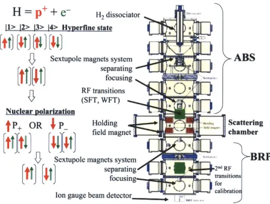
of the p+C elastic scattering reaction, which must be determined experimentally [26]. The absolute polarization is measured by Polarized Atomic Hydrogen Jet Target Polarimeter (H-Jet polarimeter) using proton-proton elastic scattering on a

transver-sly polarized proton target

[261.

the target and beam polarizations because the particles are identical and satisfy the equation:

AN ^ Etarget _ Ebeam

target Pbeam

where e is the raw asymmetry and P is the polarization. The beam polarization can therefore be measured according to

Pbeam = -Ptarget ebeam ₆ (2.4)

target

so long as the target polarization Parget is well calibrated. Because the H-Jet

po-larimeter uses protons for both the beam and target, many systematic effects cancel in the ratio of raw asymmetries.

The H-Jet polarimeter was installed in March 2004 at IP 12 of the RHIC ring, where the 3000 kg apparatus sits on rails allowing it to move 10 mm in either direction

H

p*+

e-

Sextupole magnets system

ABS

separating focusing RF transitions (SFT, WFT) Nuclear polarization

{P+

]4

[Jj

field magnet

chamber

Sextupole magnets system

separating2nd RF

focusing transitions

ABS

transition

Ion gauge beam detector _c

Figure 2-4: A diagram of the H-Jet polarimeter.

along the x-axis (horizontal, perpendicular to the beam axis). The device is made up of three sections, the atomic beam source (ABS), the scattering chamber, and the Breit-Rabi Polarimeter (BRP). A diagram of the polarimeter is included as Fig. 2-4. In the ABS, the polarized atomic beam is produced with a 6.5 mm FWHM. The beam intensity in the scattering chamber was measured to be 1.2 x 1017 atoms/s in the

commissioning run in 2004, resulting in a target thickness of 1.3 x 1012 atoms/cm2_.

The BRP measured an effective target polarization of 92.4%.

The recoil spectrometer detects the recoil proton from the elastic scattering event using three pairs of silicon strip detectors that cover 150 in azimuth centered on the horizontal plane about 80 cm from the beam. Each detector consists of 16 strips oriented vertically, providing 5.5 mrad coverage in polar angle. The kinetic energy of the recoil is calculated using the time-of-flight relative to the bunch crossing time given by the RHIC clock.

of the recoil proton. By measuring the raw asymmetry for both the beam and target, according to the formula [26]:

NL - Nri - NR Nf

E = (2.5)

NT -Nf + N N

with the event yields sorted by spin state (up-down) and detector side (left-right), it is possible to calculate the beam polarization according to Eq. 2.4. This measure-ment is used to provide the absolute polarization, to which the CNI polarimeters are normalized.

2.2

STAR

Calorimetry provided by the Barrel Electromagnetic Calorimeter (BEMC) and

track-ing providtrack-ing by the Time Projection Chamber

(TPC)

units of pseudorapidity form the core of STAR's ability to reconstruct jets over a large acceptance. The BEMC is also used for the trigger at level 0 and level 2 along with the Beam-Beam Counters (BBCs). The BBCs also record the relative luminosity, which is vital to the measurement of asymmetries in STAR.

2.2.1

BEMC

The BEMC [27] is a lead-scintillator sampling calorimeter covering 27r in azimuthal

angle

#

0.05 by 0.05 in q-# space. The towers in turn are grouped into 120 modules that each cover 0.1 in azimuth and one unit of pseudorapidity (2 by 20 towers). The BEMC surrounds the TPC, starting at a radius of approximately 225 cm and extending approximately 30 cm where it terminates upon reaching the STAR solenoid.

Each module of 40 towers is constructed of 21 mega-tiles of scintillator, interleaved with 20 plates of lead absorber. A cross section of a tower showing the layout can be seen in Fig. 2-6. The mega-tiles are each divided into 40 optically isolated tiles

n=-1 =

Bluew

BEMCn

Be BBC jOO,.Yellow

East

Figure 2-5: A diagram of the STAR detector with the primary detectors used for the jet analysis labeled.

corresponding to the towers of that module using a groove machined into each layer and filled with an opaque silicon dioxide epoxy. A black line painted on the uncut

scintillator reduces optical cross talk to less than 0.5 %. The two front scintillator

layers are 6 mm thick; the remaining scintillator and lead layers are 5 mm thick. This extra thickness is needed because these two layers are used for a pre-shower detector and have a double readout. The scintillator layers are read out using a wavelength shifting fiber embedded into a o groove in each tile.

The fibers for each tower terminate in a multi-fiber optical connector at the back of the module and the light is carried out through a 2.1 m long multi-fiber optical cable where the light from the 21 scintillator tiles is combined onto a photomultiplier tube (PMT) through a Lucite light mixer.

The PMTs are Electron Tube Inc. model 9125B with 11 dynodes and mean quantum efficiency of 13.3% with a standard deviation of 1.3%. Quality assurance tests performed on the PMTs after delivery verified that all PMTs had a quantum

239.92mm 193.04mm -- --- r -- I r=2629.99mm huullinear beammunime 91.99mm

24.99mm plat-arriage intrfae plate

plate Gompression ... plate key washen strap T.=ad plate Scintillator tile 302.99mm

-Jlir" Wa4 T"eaream aEErQMasmesass

- - --- 2235

228.16mm

Figure 2-6: A cross section of a BEMC module showing the mechanical assembly of a tower including the compression components and the location of the shower maximum detector.