HAL Id: insu-02932979
https://hal-insu.archives-ouvertes.fr/insu-02932979
Submitted on 8 Sep 2020
HAL is a multi-disciplinary open access
archive for the deposit and dissemination of
sci-entific research documents, whether they are
pub-lished or not. The documents may come from
teaching and research institutions in France or
abroad, or from public or private research centers.
L’archive ouverte pluridisciplinaire HAL, est
destinée au dépôt et à la diffusion de documents
scientifiques de niveau recherche, publiés ou non,
émanant des établissements d’enseignement et de
recherche français ou étrangers, des laboratoires
publics ou privés.
Determination of the electron anomalous mobility
through measurements of turbulent magnetic field in
Hall thrusters
A. Lazurenko, Thierry Dudok de Wit, Claude Cavoit, Vladimir
Krasnoselskikh, André Bouchoule, Michel Dudeck
To cite this version:
A. Lazurenko, Thierry Dudok de Wit, Claude Cavoit, Vladimir Krasnoselskikh, André Bouchoule, et
al.. Determination of the electron anomalous mobility through measurements of turbulent magnetic
field in Hall thrusters. Physics of Plasmas, American Institute of Physics, 2007, 14 (3), pp.033504.
�10.1063/1.2535813�. �insu-02932979�
Phys. Plasmas 14, 033504 (2007); https://doi.org/10.1063/1.2535813 14, 033504
© 2007 American Institute of Physics.
Determination of the electron anomalous
mobility through measurements of turbulent
magnetic field in Hall thrusters
Cite as: Phys. Plasmas 14, 033504 (2007); https://doi.org/10.1063/1.2535813
Submitted: 06 October 2006 . Accepted: 17 January 2007 . Published Online: 05 March 2007 A. Lazurenko, T. Dudok de Wit, C. Cavoit, V. Krasnoselskikh, A. Bouchoule, and M. Dudeck
ARTICLES YOU MAY BE INTERESTED IN
Tutorial: Physics and modeling of Hall thrusters
Journal of Applied Physics 121, 011101 (2017); https://doi.org/10.1063/1.4972269 Magnetic shielding of a laboratory Hall thruster. II. Experiments
Journal of Applied Physics 115, 043304 (2014); https://doi.org/10.1063/1.4862314 Magnetic shielding of a laboratory Hall thruster. I. Theory and validation
Determination of the electron anomalous mobility through measurements
of turbulent magnetic field in Hall thrusters
A. Lazurenkoa兲
ICARE, CNRS, 45071 Orléans, France
T. Dudok de Wit, C. Cavoit, and V. Krasnoselskikh
LPCE, CNRS and Orléans University, 45071 Orléans, France
A. Bouchoule
GREMI Laboratory, CNRS and Orléans University, 45067 Orléans, France
M. Dudeck
ICARE, CNRS, 45071 Orléans, France
共Received 6 October 2006; accepted 17 January 2007; published online 5 March 2007兲
Measurements of the turbulent magnetic field in a Hall thruster have been carried out between 1 kHz and 30 MHz with the aim of understanding electron transport through the magnetic field. Small detecting coils at the exit of the accelerating channel and outside of the ionic plume were used to characterize various instabilities. The characteristic frequencies of the observed power spectral densities correspond to known classes of instabilities: low frequency 共20–40 kHz兲, transit time 共100–500 kHz兲, and high frequency 共5–10 MHz兲. A model of the localized electron currents through a magnetic barrier is proposed for the high-frequency instability, and is found to be in good quantitative agreement with the observations. Based on the measured high-frequency turbulent magnetic field, the turbulent electric field is estimated to be about 1 V / cm outside of the plume and ranges from 10 to 102V / cm at the channel midradius at the exit of the thruster. The “anomalous”
electron collision frequency, related to the high-frequency instability, is estimated to be⬍106s−1,
which largely exceeds the classical frequency in the core of the exit plasma but is lower than the frequency that is generally used in hybrid codes. © 2007 American Institute of Physics.
关DOI:10.1063/1.2535813兴
I. INTRODUCTION
The Hall thruster is a space propulsion technology that was initially developed in the 1970s in the frame of the So-viet space program1,2 and which is frequently used today by geostationary satellites for North-South and East-West station-keeping共see, for example, Ref.3兲. Recently, this type
of thruster was implemented as the main propulsion on the interplanetary mission “SMART-1.”4
The Hall thruster is a plasma device that is based on the so-called ion accelerator with closed electron drift. A mostly radial magnetic field B is created across an annular ceramic channel, with a maximum intensity near the channel exit. The value of magnetic field is chosen in such a way that the electron Larmor radius is much smaller than the channel di-mensions, whereas the ion Larmor radius is much larger. The electrons are therefore magnetized but the magnetic field does not affect ion motions. The dc discharge voltage Ud is
applied between an anode, located at the bottom of the chan-nel, and an external hollow cathode. A propellant共xenon兲 is injected through the anode structure. The reduction of longi-tudinal mobility of electrons across the radial magnetic field leads to a localized axial voltage drop of the order of the
anode-cathode discharge voltage. In such an “E cross B” configuration, electrons drift in the azimuthal direction with an average azimuthal velocity Ez/ Br. Typical values of
Ez共104 V / m兲 and Br共20 mT兲 lead to average electron
ener-gies higher than 10 eV and this magnetically confined elec-tron cloud is very efficient for ionizing the propellant gas. The ions are accelerated toward the exit by the electric field, leaving the channel with kinetic energies of the order of the discharge potential. The thrust corresponds to the momentum delivered to this escaping ion flow. A detailed description of Hall thrusters can be found in Refs.1,2, and 5.
One of the key questions of Hall thruster physics is the understanding of electron transport through the magnetic field. Classical diffusion approaches fail to give a satisfac-tory agreement with the experiment. A correct description of the electron transport, however, is very important for making numerical codes progress toward fully predictive codes. Hybrid-type codes, for example, where electrons are de-scribed as a fluid and ions as particles, use artificial viscosity and the diffusion coefficients are chosen to properly describe macroscopic plasma motions.6–11The determination of these coefficients is a crucial problem for these simulations. Two hypotheses are generally proposed to explain this “anoma-lous” electron transport: the so-called “near-wall” conductiv-ity, where the electron collisions with walls increase the ef-fective collision frequency, and an oscillation-assisted 共or
a兲Electronic mail: [email protected]
PHYSICS OF PLASMAS 14, 033504共2007兲
turbulent兲 electron transport.1,2,12
While inside the accelerat-ing channel these two mechanisms can compete with each other, outside only the latter can exist.
One of the approaches for determining the electron transport coefficients experimentally is to measure the local time-averaged plasma properties and to deduce the electron mobility from the electron current equation.13,14Another way consists in studying the properties of the plasma oscillations and deducing the “effective” electron collision frequency from the analysis of the oscillation intensities.13,15,16 While the first approach does not differentiate between the two anomalous electron transport mechanisms, the second one informs only on the turbulent transport. Meanwhile, the sec-ond approach provides insight into the way turbulent trans-port works.
The gas discharge in Hall thrusters generates a number of plasma instabilities whose intensities depend strongly on the thruster operating parameters, notably the discharge volt-age and the magnetic field.1,2,12 Numerous techniques have been implemented to study experimentally the physics of Hall thrusters, and in particular plasma instabilities. Ex situ diagnostics include the observation of instability signatures in the electric power circuit, or the space-averaged detection of light emission from the channel and plume. In situ diag-nostics, in the thruster channel and in the thruster plume, include electric probes, arrays of optical fibers, the imple-mentation of time-of-flight techniques and special discharge interrupters, or inductive coils. A comprehensive review of physical insight obtained with these different techniques is given in Ref.17.
The detection of magnetic fields generated by charged particle currents in the Hall thruster plasma provides impor-tant insight into thruster physics, and especially into nonsta-tionary processes. A wire loop around the channel circumfer-ence was used in a number of previous investigations to record the variation of magnetic field from the electron azi-muthal drift current and to investigate its spatial and tempo-ral evolution.17–20Magnetic probes are widely used in differ-ent laboratory plasma devices, in particular in magnetized plasma accelerators共see, for example, Ref.21兲.
In this paper, we present an implementation of the mag-netic field detection technique for studying plasma instabili-ties in Hall thrusters. This diagnostic is based on the local-ized共in azimuth, axial, and radial directions兲 detection of the time-varying magnetic field generated in the plasma volume. The driving interest is to shed light on the generation mecha-nism of instabilities in the 5 – 10 MHz frequency range,2,12,22–27 and to evaluate from this the diffusion coeffi-cient that would be needed for hybrid codes. Meanwhile, we found out that this technique is also suitable for studying different types of instabilities in the wide frequency range.
This paper is organized as follows. In Sec. II, a descrip-tion of the experimental setup is given. In Sec. III, the ex-perimental results are presented, which are followed by a more detailed interpretation in Sec. IV. The conclusions are formulated in Sec. V.
II. EXPERIMENTAL SETUP A. Principle of diagnostics
A nonstationary magnetic field generates a voltage drop in a coil positioned in such a way that the force lines cross the coil surface. The underlying effect is described by Fara-day’s law,
= −d⌽
dt , ⌽ = NSB, 共1兲
where is the electromotive force 共voltage generated in the coil兲, ⌽ is the magnetic flux crossing the coil surface, N is the number of turns in the coil, S is the coil surface, and B is the magnetic induction. With a properly oriented coil axis, it is possible to detect selectively the variations of any compo-nent of a nonstationary magnetic field. Such a coil has a linear frequency response. Indeed, for a magnetic field that is generated by the current flowing in an infinitely long straight wire,
B =0
I
2r, 共2兲
where is the relative magnetic permeability, 0= 4
⫻10−7H / m, I is the intensity of the current in the wire, and
r is the distance from the wire. With the ansatz I = I0e−jt,
then = −d⌽ dt = j0 NS 2rI = j0f NS r I, 共3兲
and is therefore a linear function of the frequency f. Such coils are routinely used for investigating ionospheric plasmas.28,29
B. Configuration of the measurement system
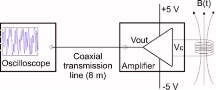
The detecting coil diameter was chosen a priori to be equal to 9 mm, resulting from the tradeoff between a com-pact size and easiness in fabrication and handling. To define the shape of the measurement system, let us assume that the typical discharge current of 4.2 A is concentrated on the thruster axis and oscillates at the 20 kHz frequency of the bulk instability.1,2,12Then, according to Eq.共3兲, the magnetic field from this current induces the voltage drop of⬃100V in the 9 mm coil of one turn, located at r = 50 mm from the thruster axis. Each coil should therefore have several turns to increase the signal level and should be closely followed by an amplifier to avoid signal degradation 共Fig. 1兲. Such a
design is inherited from the instrumentation for ionospheric investigations.29
The coils are built from ordinary 0.8 mm enameled transformer wire. Each coil has 18 turns 9 mm in diameter with overall longitudinal dimension of 7 mm. The length of the coil’s free ends is 80 mm. The measured self-inductance of the coils is on the order of 2.3H at 10 kHz.
The amplifiers are mounted on a printed circuit board 共PCB兲, with two amplifiers on each PCB 共one amplifier for each coil兲. The 50 ⍀ output impedance of the amplifiers is adapted to the transmission lines, using a SMA connector to connect the cables to the PCBs. The signals are transferred through 8 m coaxial lines and are observed and recorded on the digital four-channel Tektronix 5104B oscilloscope.
C. Calibration of coils and amplifiers
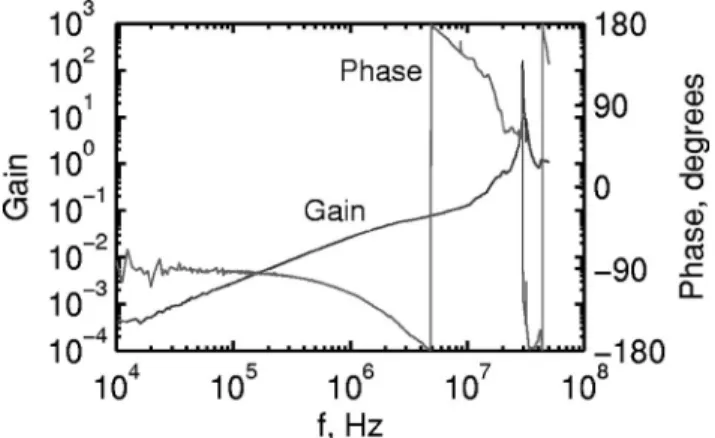
The amplifiers were first calibrated separately from the coils by applying on the input a sinusoidal voltage of vari-able frequency in the 103– 107Hz range. The amplifier gain is quite flat共90–100兲 up to 106Hz, whereas for high frequen-cies of 107Hz it drops to⬃60 共Fig.2兲. The amplifiers also
shift the phase at high frequencies共see Fig.2兲.
The coils and the amplifiers were then calibrated to-gether according to the following scheme 共Fig. 3兲: a long
metallic bar was inserted into a circuit carrying a sinusoidal current of variable frequency. The coils were placed at 50 mm from the bar with the surface of the coil perpendicu-lar to the magnetic field. The amplifier output voltage Uacq was compared to the input voltage Ugen to get the transfer function of the system. The resulting Bode plot is presented in Fig.4. Notice a resonance at 30 MHz.
The gain of the system “coil+ amplifier” can be repre-sented as
Gain = Gain共兲 =Uacq
Ugen
= Uacq
IgenR50⍀
, 共4兲
whereis the pulsation. Taking into account Eq.共2兲for the magnetic field of a long wire, one can write the magnetic field as
B共兲 = Uacqftr共兲, 共5兲
where ftr共兲 is the “effective” transfer function,
ftr共兲 =
1
20dR50⍀Gain
. 共6兲
D. Installation on the thruster
The measurements were carried out on the Hall thruster SPT-100ML at the French national facility PIVOINE.30 The thruster operated at its nominal operation mode, with a mass-flow rate of 4.5 mg/ s, a discharge voltage of Ud= 300 V, and
a discharge current of Id= 4.2 A.
Three coils were installed at the thruster exit in front of the external magnetic pole around the channel共Fig.5兲 on a
radius 70 mm. The axes of two coils共B7 and B3 on Fig.5兲
were oriented azimuthally, and the last coil B6 was oriented
FIG. 2. 共Color online兲 Amplifier characteristics.
FIG. 3. Scheme of the amplifier and coil calibration setup.
FIG. 4. Frequency characteristics of the “coil+ amplifier” system. This sys-tem has a resonance at 30 MHz.
with its axis parallel to the thruster axis. Therefore, B7 and B3 detect the azimuthal component of the fluctuating mag-netic field, whereas coil B6 detects the axial component. A shielded Langmuir probe27was also installed at the same exit cross section of the thruster, and it will be referred to as A8 共see Fig.5兲. The probe operated at practically ground
poten-tial; the signal from the probe was directly observed on the oscilloscope at 50⍀ ac operation mode.
The amplifiers were installed in the lateral zones of the thruster in order to be close enough to the coils 共80 mm兲 while being protected from the excessive heat flux.
Oscillations in discharge current were also recorded us-ing Tektronix P6022 current probes installed on the power circuit.
III. RESULTS A. Coil signals
A typical coil recording is presented in Fig.6along with the wave form of the discharge current. One can directly observe the modulation of the coil signal at the frequency of discharge current oscillations at 25 kHz. There are also some intervals where the signal level strongly drops, which we attribute to the instantaneous saturation of the amplifier. Such regimes are excluded from our analysis.
We calculated the power spectral density of the raw sig-nals separately for two frequency bands:
FIG. 5.共Color online兲 Location of the magnetic field coils and the Langmuir probe on the SPT-100ML thruster.共a兲 Schematics; the B6 coil is oriented axially, while the B7 and B3 are oriented azimuthally. A8 stands for the coaxial Langmuir probe.共b兲 Picture of the SPT-100ML thruster, with the coils and the probe. Some additional diagnostics are seen that are not perti-nent for this study.
FIG. 6. Time evolution of the discharge current共a兲, a typical coil B7 signal 共b兲, and an excerpt of the same coil signal 共c兲. Notice that the coil signal has the same LF variations as the discharge current.
共i兲 For f⬍1 MHz, using Welch’s periodogram method with a single Hamming window.
共ii兲 For f⬎1 MHz using the same method, with a sliding Hamming window of 213 samples and 50%
overlapping.
Typical spectra are represented in Fig.7for the coils B3, B6 and for the Langmuir probe A8. The spectrum of the B7 coil is close to that of the B3 one and is not shown. Three characteristic frequency bands can be distinguished in the spectra: 20– 40 kHz, 100– 500 kHz, and 8 – 24 MHz.
The 20– 40 kHz frequency range corresponds to the low-frequency共LF兲 oscillations in Hall thrusters, often referred to as “contour” or bulk oscillations.1,2,12,31 These oscillations are conventionally considered as being the most important ones and are associated with the displacement of the ioniza-tion front;32they are synchronous in the whole plasma vol-ume. The modulation of the discharge parameters at these frequencies can reach up to 100%; usually, the values are significantly lower by adjustment of the magnetic field, and therefore do not affect the operation of the thruster.2 In our experiment, the orientations of the coils suggest that different physical sources contribute to the coil signals of B3 and B7 on the one hand and to B6 on the other hand. Coils B3 and B7 detect the azimuthal magnetic field that is generated by currents of charged particles having axial and radial compo-nents. These currents are carried by ions leaving the thruster, which have significant axial and radial components and neg-ligible azimuthal component, and corresponding components of electron current. These currents are modulated at a LF scale. Coil B6 detects the axial magnetic field that is gener-ated by azimuthal and radial currents. Such currents are made out of the radial components of ion and electron cur-rents and the azimuthal component of electron current, which is referred to as Hall current. Numerous studies show17–20 that the Hall current is several times greater than the
dis-charge current and is also modulated at the LF scale. Therefore, it is reasonable to suggest that the Hall current is a main physical source of signal for axially oriented coils such as B6.
The 100– 500 kHz frequency range corresponds to the “transit-time” 共TT兲 oscillations in Hall thrusters, which are usually related to the ion passage through the channel;1,2,12,33 some reports extend the upper limit of these oscillations to several MHz.2According to some studies,2the TT instability could be quite intense, but to our knowledge there have been no reports on the significance of oscillations in this fre-quency range, in Hall thrusters that are currently under de-velopment. The B6 spectrum in this 100– 500 kHz frequency range is flat, in contrast to the spectra of B3 and A8共see Fig.
7兲. This observation corroborates the hypothesis of ion
mo-tion being responsible for TT oscillamo-tions. The ion current has a mostly axial direction, thus generating an almost azi-muthal magnetic field that is detected by coils B3 and B7.
FIG. 8. 共Color兲 Cross-correlation function for the B3 and B7 coils. The offset of the maxima in the cross-correlation共red color兲 relative to the time lag on the vertical axis indicates a time shift between the signals.
FIG. 9. 共Color兲 Dispersion relation estimated from coils B3 and B7. The vertical scale corresponds to the logarithm of the power spectral density. The periodicity in k is a consequence of the Nyquist limit. The wave number k is normalized with respect to the value corresponding to a dipolar structure. The alignment of the maxima along a line going through共= 0, k = 0兲 attests to a dispersionless motion.
FIG. 7.共Color兲 Power spectral densities of the coil signals and of the probe signal. Left panels for f⬍1 MHz and right panels for f ⬎1 MHz. Logarith-mic scales are used for the axes.共a兲 shows low-frequency spectra from coil B3共black兲 and B6 共red dashed兲. Notice a relative depletion of the spectrum of B6 in the 100– 500 kHz range.共b兲 shows the low-frequency spectrum of the A8 probe.共c兲 shows high-frequency spectra of coils B3 共black兲 and B6 共red dashed兲, with similar spectra. 共d兲 shows the high-frequency spectrum of the A8 probe.
Fluctuations in this frequency range are also present in Lang-muir probe spectra, thereby suggesting that various plasma parameters change on this time scale. Taking into account the linear frequency response of coils关see Eq.共3兲兴, we conclude that the TT oscillations are weaker than the LF ones in this thruster operation mode.
Our high-frequency band is limited here at 30 MHz be-cause of the coil resonance and the unstable operation of the electronic components. Frequencies between 5 and 30 MHz correspond to the high-frequency共HF兲 oscillations that have attracted much attention in the past22,23 and again recently.24–27Such HF instabilities generate azimuthal waves that propagate with velocities close to the electron drift ve-locity 共⬃106m / s兲 in the crossed electric and magnetic fields.22–27 The impact of instabilities in the HF frequency range on particle diffusion was recently unambiguously dem-onstrated in fully kinetic numerical simulations.34 Figure 7
shows a strong correlation between the HF spectra of the Langmuir probe and the three coils. The cross-correlation function of B7 and B3 signals, obtained with a rectangular moving window of 210samples with 50% overlapping, gives
a signal time shift on the order of 50 ns共Fig.8兲. This
indi-cates that the source propagates in the azimuthal direction with a velocity of about 2⫻106m / s. The same velocity can
be obtained from the autocorrelation functions of each coil and the Langmuir probe. These observations are in perfect agreement with recent studies with the help of antennas and probes.24–27The close properties of coil and probe signals in the time and frequency domains already suggests a common underlying physical process, to be discussed below.
We also analyzed the HF component of the coil signals by making use of wavelets, which are better suited for the study of such a quasistationary wave-field. From this we can estimate the power spectral density versus pulsation and wave number k.35A linear dispersion relation is found, see Fig. 9. In the same figure, domains where the coherence between the signals is below 0.75 are left in white. From the linear dispersion relation, we conclude that the plasma per-turbations rotate azimuthally as a rigid body.
B. Magnetic field
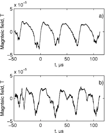
We deduced the value of induced magnetic field outside of the channel共at the location of the coils兲 by applying the transfer function obtained from the calibration关see Eq. 共6兲兴. The magnetic field is modulated at the LF scale with an amplitude of about 10−5T 共Fig. 10兲. This value is several
orders of magnitude lower than the stationary magnetic field of the thruster magnetic system: about 0.015 T in the chan-nel and 0.02 T at the detecting coils positions. Nevertheless, in the core of the plasma region that stretches from a few mm inside to a few mm outside the channel, the induced mag-netic field could be significantly higher. A simple 1 / r spatial variation, suggested by Eq.共2兲, leads to rather high induced fields there, at the axial location of coils, assuming a radial location of the field generating current somewhere within the core. This is coherent with other studies reporting a one or-der of magnitude only lower induced magnetic field near the exit of the channel.20,36
The HF component of magnetic field was extracted by applying a digital Butterworth high-pass filter with a cutoff frequency of 2 MHz. Some examples of the filtered data are shown in Fig.11. The HF component of the magnetic field is one order of magnitude weaker than the LF component.
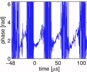
The phase difference between the axial and azimuthal components of the magnetic field is presented in Fig. 12. Notice periodic variations of the phase difference between 1.5– 3.5 rad, which are caused by the LF modulation 共see Fig. 6兲. Unfortunately, it is impossible to reconstitute the
exact direction of the induced magnetic field without the third r component.
IV. INTERPRETATION
The amplitude of the induced magnetic field that is mea-sured outside of the channel is three to four orders of mag-nitude lower than the continuous magnetic field共⬃10−2T兲.
As we shall see, however, this induced magnetic field is very important for electron diffusion, and allows the electron dif-fusion coefficients to be evaluated. The locally measured in-duced magnetic field in addition provides valuable informa-tion on the current distribuinforma-tions and thereby on charged particle motions in the Hall thruster. We just saw that the spectral characteristics of the wave-field correspond well to known classes of oscillations in Hall thrusters. The origins of LF 共20–40 kHz兲 and TT 共100–500 kHz兲 phenomena are more or less understood through numerous experimental, theoretical, and numerical studies.1,2,12,31–33 A less studied
part of magnetic field spectra concerns HF oscillations above 5 MHz, which are limited in our case to 30 MHz by the diagnostics.
We will consider two models in an attempt to understand the generation mechanism of the HF magnetic field. The first of them is related to the hypothesis of local electron density perturbations moving in the azimuthal direction with a ve-locity close to the electron drift veve-locity.24,26,27The second is inspired from speculations that the HF instability may induce a sufficient number of anomalous electron collisions for gen-erating a notable perpendicular electron transport共discussed later in this section兲. Since the HF instability is suggested to be localized in azimuthal and axial directions,26 this perpen-dicular electron transport could be represented by a system of localized electron currents. This instability arises in the plasma volume and it has been found to be the strongest at the exit part and outside of the channel. Therefore, our mod-eling will deal with the electron transport outside of the channel and that part of the anomalous transport inside the channel that is due to plasma turbulence.
Magnetic fields in plasmas are generated by charged par-ticle currents as described by the Maxwell equation,
ⵜ ⫻ Hជ= Jជ+Dជ
t , 共7兲
where H is the magnetic field, J is the charged particle cur-rent density, and D is the electric field. In the case of Hall thrusters, the charged particles—electrons and ions—move with velocities well below the speed of light c. These veloci-ties could be directly estimated from the characteristic dis-charge voltage 300 V. In reality, electron characteristic ve-locities are even smaller because electrons are effectively trapped by magnetic field. Electron drift velocities in crossed electric and magnetic fields are of the order of 106m / s for a magnetic field of 20 mT and an electric field of 104V / m. Therefore, particle movement is nonrelativistic and the rela-tivistic effects can be neglected here. We will also neglect displacement currents.
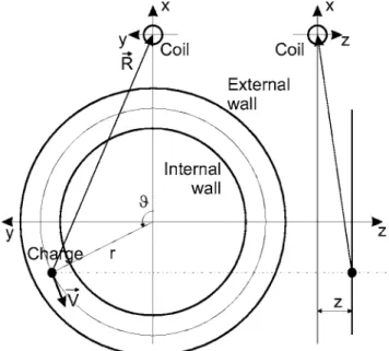
A. Magnetic field from the localized charge
Let us consider a point charge located on the middle radius of the accelerating channel 共in the case of a SPT-100ML thruster, the radius is 42.5 mm兲 and turning with the pulsation= 2f corresponding to the first HF spectral peak f = 8 MHz共see Fig.7兲. The axial propagation velocity of the
charge is zero. We simulated the motion of such a charge using Liénard-Wiechert potentials,37
= 1 40 e
冉
R −vជRជ c冊
, Aជ= 0 4 evជ冉
R −vជRជ c冊
, 共8兲where is the electric potential, Aជ is the vector potential,vជ
is the charge velocity, and R is the distance from the charge to the observation point. The magnetic field H is calculated according to
Hជ= rotAជ. 共9兲
FIG. 12.共Color online兲 Phase shift between the axial and azimuthal com-ponents of the magnetic field共coils B6 and B7兲. Periods with rapidly chang-ing values coincide with the absence of correlation between signals in the HF domain共sometimes because of a saturation of the amplifiers兲 and should therefore be discarded.
FIG. 11.共Color online兲 共a兲 HF component of a magnetic field; 共b兲 excerpt of the coil signal;共c兲 excerpt of the probe signal.
The calculation scheme is presented in Fig.13. The mag-netic field was calculated at the actual location of the detect-ing coil, i.e., at Rc= 70 mm, assuming its axial position is the
origin of axial coordinate共z=0 mm兲 and coincides with the thruster exit. The value of electric charge was adjusted to obtain the experimental values of magnetic field 共see Figs.
10and11兲. With such charges, the calculated azimuthal
mag-netic field Bis much smaller than the axial one Bz共Fig.14兲.
This could be changed with charges moving far away from the detecting coil. The phase relation between the azimuthal and axial magnetic fields, however, does not agree with the observations共see Fig.12兲. Furthermore, the axial position of
the rotating charge is limited to a few cm outside of the channel because of the rapidly decreasing electric field共see, for example, Refs.1,2, and5兲, which leads to the
cancella-tion of azimuthal electron drift. Therefore, the hypothesis of a localized charge moving azimuthally cannot reproduce well the observed picture.
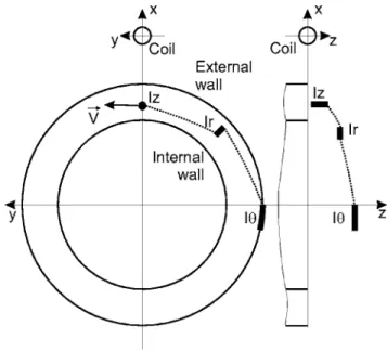
B. Magnetic field from the localized currents
Let us now consider in the plasma volume a system of localized currents of the charged particles, modeled by infi-nitely thin wires of finite length. The currents can be oriented in an arbitrary manner, but the whole current system is sup-posed to turn around the center of the channel as a rigid body with the frequency = 2f corresponding to the first HF
spectral peak f = 8 MHz. The contributions to the magnetic field were calculated separately for each current and then added to obtain the resulting field. The calculation was done with the help of the vector potential Aជ,
Aជ= 0 4
冕
I
ជ
RdL, 共10兲
where Iជ is the current of charged particles, and dL is the infinitely small linear element of the current. The magnetic field is again calculated according to共9兲 at the location Rc
= 70 mm, z = 0 mm, coinciding with the thruster exit plane. For simplicity, three types of elementary currents are considered: an axially oriented current Iz, an azimuthal
cur-rent I, and a radial current Ir. The absolute value of all the
currents was chosen to be equal to the estimated electron current through the magnetic barrier, i.e., corresponding to a discharge current of Id= 4.2 A, the values of elementary
cur-rents were taken to be 0.2⫻Id. Azimuthal B and axial Bz
components of the magnetic field from each elementary cur-rent are presented in Figs.15共a兲–15共c兲. It can be seen that the sole axial current Iz关Fig.15共a兲兴 cannot reproduce the
experi-mentally observed HF magnetic field共see Fig.11兲. A closer
matching could be obtained by adding azimuthal关Fig.15共b兲兴 and radial 关Fig. 15共c兲兴 currents. Actually, these elementary currents, when placed in the limits of the assumed electron turbulent transport zone 共r=3.5–8 cm, z=0–3 cm兲, defined by the channel dimensions and the relative cathode-channel position, give a correct order of magnitude for the magnetic field. To obtain a correct phase relation, however, these el-ementary currents should be shifted azimuthally relatively to each other. For example, the resulting magnetic field shown in Fig.15共d兲 corresponds to the configuration given in Fig.
16. This configuration gives a phase shift between resulting z and components of about/ 2, which agrees with the ex-perimentally observations共see Fig.12兲. Such a configuration
can model a spiral-like current that starts outside the channel close to the cathode radial and axial position and flowing into the channel, at the same time rotating with a velocity close to the electron drift one. In this example, the elemen-tary currents are not connected; their possible connections are shown by dashed lines. Accounting for these connections will of course change the resulting magnetic field. Notice, however, that the localized current approximation is a rather strong one, since the real currents in the plasma volume have a certain distribution and their directions can deviate from being strictly axial, azimuthal, or radial.
A more consistent reconstruction of plasma volume cur-rents could be obtained with a thorough experimental map-ping of the turbulent magnetic field, in particular with the help of intrusive probing. This, however, would bring
addi-FIG. 13. Scheme of magnetic field calculation from a point charge.
FIG. 14.共Color online兲 Magnetic field simulated for an azimuthally moving charge.
tional perturbations to the discharge. At this point, we pro-pose to consider our model as a phenomenological one, not intending to get the exact current reconstruction. Although this model lacks solid theoretical proof, it agrees quantita-tively with the experimental picture. This model is also co-herent with the subsequent derivation of the electron “effec-tive” collision frequency.
C. Relation to the electron transport
Theoretical studies23,33,38,39 predict the existence of un-stable modes in all the above discussed frequency ranges, but according to fully kinetic simulations,34it is an instability in the MHz range that leads to the generation of the azimuthal turbulent electric field and to the “anomalous” electron trans-port. Our experiments and the earlier works22–27 have confi-dently identified the azimuthal wave with a fundamental fre-quency f⬇5–10 MHz, though with generally low wave numbers k⬃20 to 200 m−1. We will now proceed with the
analysis of this instability in order to estimate an “effective” electron collision frequency.
The plasma conditions in the thruster are ⍀eⰆp, e,i=0
2kBnTe,i
B2 Ⰶ 1, 共11兲
where⍀e,pare the electron gyro and plasma frequencies,
Te⬃5 eV, TiⰆTeare, respectively, the electron and ion
tem-peratures, and n⬃1017m−3is the electron density at the exit
of the thruster. The high-frequency waves of interest are in the frequency range between electron and ion gyrofrequen-cies⍀iⰆⰆ⍀e and are supposed to propagate almost
per-pendicularly to the ambient magnetic field k⬜Ⰷk储. Such
azi-muthal waves belong to so called quasi-electrostatic waves in low hybrid frequency range. Their frequency dependence is described by the following relation:40,41
2= ⍀e2k2c2 p 2
冉
1 +k 2c2 p2冊
冤
m+ cos2 k2c2 p 2冉
1 +k 2c2 2p冊
冥
, 共12兲wherem= me/ Miis the electron to ion mass ratio and is
the angle between the direction of magnetic field and the direction of wave propagation. In these oscillations, the elec-trons are magnetized while the ions are not, k⬜eⰆ1 and
k⬜iⰇ1, where e andi are, respectively, the electron and
FIG. 15. 共Color online兲 Magnetic field simulated for localized plasma cur-rents:共a兲 from an axial current, 共b兲 from an azimuthal current, 共c兲 from a radial current,共d兲 sum of all contributions.
FIG. 16. Configuration of elementary currents, corresponding to Fig.15; bold, length of the currents for simulation in Fig.15; dashed, possible con-nections between the currents; direction of rotation is shown共vector V兲. 033504-9 Determination of the electron anomalous mobility… Phys. Plasmas 14, 033504共2007兲
ion Larmor radia. These waves were shown to be generated in Hall thrusters due to the resistive instability studied by Litvak and Fisch.38
These quasi-electrostatic waves are known to play an important role in space plasmas in particle transport and ac-celeration; they are observed in the polar ionosphere and in the vicinity of quasiperpendicular collisionless shocks,41,42 where they are supposed to play an important role in particle acceleration. The particularity of wave particle interaction for these waves consists in the fact that electrons in these motions are magnetized while ions are not. As a conse-quence, electron motion is mostly affected by the electric field component parallel to the background magnetic field, while ions interact with the major component of the electric field. Because of this, these waves can transfer momentum from parallel electron motion to perpendicular ion motion and vice versa. In the presence of an external electric field, which is the case here, energy can also be transferred. A theoretical study of these waves is beyond the scope of this paper, so we will use known formulas from the literature to evaluate the “effective” collision frequency. This character-istic “effective” or “anomalous” collision frequency can be deduced from direct in situ measurements of magnetic field fluctuations.
The rate of the electron momentum loss due to the gen-eration of waves can be estimated as follows:
effmenVd= − Ffr, 共13兲
where eff is the “effective” collision frequency, Vd is the
characteristic drift velocity of electrons, n is their density, and Ffris the characteristic friction force that appears due to
the instability with respect to the generation of waves. This friction force can be evaluated as follows:15,16
Ffr= 2
共2兲3
冕
␥kWkk
k
d3k, 共14兲
where␥kis the increment of the instability due to the
elec-tron drift motion that is responsible for the instability gen-eration. Thus this “effective” frequency can be estimated as follows: eff= 2 共2兲3m enVd2
冕
␥kWk k k d3k. 共15兲When the electrons are magnetized and ions are not, the macroscopic motions of electrons can be determined by the “effective” diffusion, and ion motion is governed by the macroscopic electric fields. The perpendicular diffusion co-efficient for electron motions in this case can be derived from the “effective” collision frequency as D⬜=effe2 and it can
be evaluated if the level of wave activity W =兰Wkd3k and the
characteristic increment are known. The level of wave activ-ity can be estimated from the wave electric field Wk
=0E2/ 2. To estimate the characteristic amplitude of the
electric field, we make use of Ampere’s law共7兲, neglecting the displacement current, and taking the estimate of the perpendicular 共“anomalous”兲 current density, assuming that it is carried mostly by electrons, J⬜= −enVe⬜
= −en共兩␦Eជ⫻Bជ0兩/B02兲⬇−en共␦E / B0兲, where␦E is the
fluctuat-ing 共turbulent兲 electric field that is assumed to be perpen-dicular to the stationary magnetic field B0. From共7兲we have
兩ⵜ⫻␦Hជ兩=兩共1/0兲ⵜ ⫻␦Bជ兩⬇共1/0兲k␦B, where␦B is the
tur-bulent magnetic field and k is the wave number. This leads to the following relation between the fluctuating magnetic and electric fields: ␦E⬇⍀e p2 k 00 ␦B, 共16兲
where k is the wave number of the experimentally detected azimuthal HF wave. In the simplest case, its wavelength is equal to the channel circumference 2R, but as was
demon-strated in Refs.26and 27, these HF waves can have much smaller wavelengths共down to at least 1 cm兲, which leads to
k⬃共0.2–6.3兲⫻102m−1. From this we get ␦E
⬃0.14–4.4 V/cm, and thus Wk/ menVd2⬇Wk/ kBnTe
⬇0␦E2/ 2kBnTe⬃10−5– 10−3. It is rather difficult to evaluate
the increment of the instability, but for rather strong devia-tions from equilibrium one can take it to be of the order of
␥k⬇0.1⫻LH= 0.1⫻⍀e共me/ Mi兲1/2⬇5⫻105s−1. In this
case, the characteristic “anomalous” collision frequency will be of the order of 5⫻102s−1. This value is significantly
smaller than “classical” collision frequency. However, this evaluation utilized the oscillation intensities measured out-side the region of denser plasma in front of the channel共cf. coil positions in Fig.5兲. Taking the calculated dependencies
of the magnetic field, one finds that the field amplitude, while approaching the core of this region, can increase by as much as 10 to 30. The effective collision frequency can therefore reach values of the order of 共5⫻104兲−共1 ⫻106兲 s−1. From this, the turbulent electric field can reach
approximately 102V / cm, which is comparable to the axial electric field. The possibility of generating such strong tur-bulent electric fields was demonstrated numerically.34 This can result in a quite strong effect as the characteristic “colli-sional” frequency in the same region of the thruster is evalu-ated to be of the order of= 105s−1. We conclude that in the vicinity of the channel, the diffusive behavior of the elec-trons is governed by turbulence, whereas in the periphery of the flow, classical collisions with neutrals prevail.
V. CONCLUSIONS
The turbulent magnetic field measurements in a Hall thruster reveal the nature of the physical processes that gov-ern electron transport. Although the turbulent magnetic field that is measured outside of the channel is too weak to affect charged particles directly, it provides relevant information on their dynamics. The characteristics of the magnetic field os-cillations we observe in the low-frequency and transit-time frequency ranges are in a good agreement with properties derived from other types of diagnostics. Magnetic field mea-surements give complementary information about ion accel-eration processes and Hall current evolution.
The basic hypothesis underlying the interpretation of the nonstationary magnetic field measurements is the generation of this field by moving charged particles in the plasma
volume. We have shown that the source of HF instabilities can be represented by localized currents with different orien-tations. This model is in good agreement with the experimen-tal results. More detailed studies with all three components of the magnetic field in principle allow the current distribu-tion to be reconstructed.
The key result of this study is the first direct experimen-tal evaluation of the “effective” or “anomalous” collision fre-quency due to the plasma turbulence in Hall thrusters. It has been shown that in the central region just outside the thruster, the electron dynamics is determined by “effective” or “anomalous” collisions associated with the plasma turbu-lence. In the periphery, however, classical collisions are more important. The effective collision frequency is found to be sufficiently smaller than the one used in computer simula-tions共see, for example, Refs.8and9兲. This “low
effective-ness” of anomalous transport processes may be one of the reasons for the strongly nonstationary dynamics of the thruster.
We have thereby demonstrated that the localized 共in axial, radial, and azimuthal directions兲 detection of the non-stationary magnetic fields represents a valuable and very im-portant type of diagnostic for probing nonstationary pro-cesses in Hall thrusters. Such a diagnostic can be both nonintrusive and intrusive.
ACKNOWLEDGMENTS
The authors acknowledge the technical support of P. Dom and the PIVOINE team: S. Sayamath, C. Legentil, and P. Lasgorceix. This work was performed in the frame of the research group GDR n°2759 CNRS/CNES/SNECMA/ Universities “Propulsion Spatiale à Plasma.”
1A. I. Morozov and V. V. Savelyev, Rev. Plasma Phys. 21, 203共2000兲. 2V. V. Zhurin, H. R. Kaufman, and R. S. Robinson, Plasma Sources Sci.
Technol. 8, R1共1999兲.
3H. Gray, S. Provost, M. Glogowski, and A. Demaire, in Proceedings of the
29th International Electric Propulsion Conference, Princeton, NJ共Electric
Rocket Propulsion Society, Worthington, 2005兲, IEPC-05–082.
4C. R. Koppel and D. Estublier, in Proceedings of the 29th International
Electric Propulsion Conference, Princeton, NJ共Electric Rocket Propulsion
Society, Worthington, 2005兲, IEPC-05–119. 5V. Kim, J. Propul. Power 14, 736共1998兲.
6K. Komurasaki and Y. Arakawa, J. Propul. Power 11, 1317共1995兲. 7J. M. Fife, Ph.D. thesis, Massachusetts Institute of Technology共1998兲. 8G. J. M. Hagelaar, J. Bareilles, L. Garrigues, and J.-P. Boeuf, J. Appl.
Phys. 91, 5592共2002兲.
9G. J. M. Hagelaar, J. Bareilles, L. Garrigues, and J.-P. Boeuf, J. Appl. Phys. 93, 67共2003兲.
10J. W. Koo and I. D. Boyd, Phys. Plasmas 13, 033501共2006兲.
11M. K. Scharfe, N. Gascon, M. A. Capelli, and E. Fernandez, Phys. Plasmas 13, 083505共2006兲.
12E. Y. Choueiri, Phys. Plasmas 8, 1411共2001兲.
13G. S. Janes and R. S. Lowder, Phys. Fluids 9, 1115共1966兲.
14N. B. Meezan, W. A. Hargus, Jr., and M. A. Cappelli, Phys. Rev. E 63, 026410共2001兲.
15A. A. Galeev and R. Z. Sagdeev, Nonlinear Plasma Theory, in Reviews of Plasma Physics Vol. 7, edited by M. A. Leontovich共Consultant Bureau, New York, 1979兲, pp. 1–180 共translated from Russian兲.
16A. A. Galeev and R. Z. Sagdeev, Current Instabilities and Anomalous
Resistivity of Plasma, in Handbook of Plasma Physics, Basic Plasma
Phys-ics, edited by A. A. Galeev and R. N. Sudan共North Holland, Amsterdam, 1984兲, Vol. 2, pp. 272–303.
17A. Bouchoule, Ch Philippe-Kadles, M. Prioul et al., Plasma Sources Sci. Technol. 10, 364共2001兲.
18V. N. Dem’yanenko, I. P. Zubkov, S. V. Lebedev, and A. I. Morozov, Sov. Phys. Tech. Phys. 23, 376共1978兲.
19A. I. Bugrova, V. S. Versotskii, and V. K. Kharchevnikov, Sov. Phys. Tech. Phys. 25, 1307共1980兲.
20C. A. Thomas, N. Gascon, and M. A. Capelli, Phys. Rev. E 74, 056402 共2006兲.
21D. C. Black, R. M. Mayo, and R. W. Caress, Phys. Plasmas 4, 3581 共1997兲.
22G. G. Shishkin and V. F. Gerasimov, Zh. Tekh. Fiz. XLV, 1847共1975兲. 23Y. V. Esipchuck and G. N. Tilinin, Sov. Phys. Tech. Phys. 21, 417共1976兲. 24M. Prioul, Ph.D. thesis, Orleans University, France共2002兲.
25A. A. Litvak, Y. Raitses, and N. J. Fisch, Phys. Plasmas 11, 1701共2004兲. 26A. Lazurenko, V. Vial, M. Prioul, and A. Bouchoule, Phys. Plasmas 12,
013501共2005兲.
27A. Lazurenko, L. Albarède, and A. Bouchoule, Phys. Plasmas 13, 083503 共2006兲.
28M. Parrot, D. Benoist, J. J. Berthelier et al., Planet. Space Sci. 54, 456 共2006兲.
29C. Cavoit, Rev. Sci. Instrum. 77, 064703共2006兲.
30A. Bouchoule, A. Cadiou, A. Heron, M. Dudeck, and M. Lyszyk, Contrib. Plasma Phys. 41, 573共2001兲.
31N. Yamamoto, K. Komurasaki, and Y. Arakawa, J. Propul. Power 21, 870 共1998兲.
32J.-P. Bœuf and L. Garrigues, J. Appl. Phys. 84, 3541共1998兲.
33S. Barral, K. Makowski, Z. Peradzynski, and M. Dudeck, Phys. Plasmas 12, 073504共2005兲.
34J. C. Adam, A. Héron, and G. Laval, Phys. Plasmas 11, 295共2004兲. 35T. Dudok de Wit, V. V. Krasnoselskikh, S. D. Bale, M. W. Dunlop, H.
Lühr, S. J. Schwartz, and L. J. C. Woolliscroft, Geophys. Res. Lett. 22, 2653共1995兲.
36P. Y. Peterson, A. D. Gallimore, and J. M. Haas, Phys. Plasmas 9, 4354 共2002兲.
37L. D. Landau and E. M. Lifshitz, The Theory of Field, 7th ed.共Nauka, Moscow, 1988兲, p. 216.
38A. A. Litvak and N. J. Fisch, Phys. Plasmas 8, 648共2001兲. 39A. A. Litvak and N. J. Fisch, Phys. Plasmas 11, 1379共2004兲.
40A. B. Mikhailovskii, Instabilities of a Homogeneous Plasma, Theory of Plasma Instabilities Vol. 1共Consultant Bureau, New York, 1974兲 共transla-tion from Russian兲.
41V. Krasnoselskikh, E. Kruchina, G. Thejappa, and A. Volokitin, Astron. Astrophys. 149, 323共1985兲.
42O. Vaisberg, A. Galeev, G. Zastenker, S. Klimov, M. Nozdrachev, R. Sagdeev, A. Sokolov, and V. Shapiro, Sov. Phys. JETP 58, 716共1983兲. 033504-11 Determination of the electron anomalous mobility… Phys. Plasmas 14, 033504共2007兲