HAL Id: hal-00318141
https://hal.archives-ouvertes.fr/hal-00318141
Submitted on 13 Sep 2006
HAL is a multi-disciplinary open access
archive for the deposit and dissemination of
sci-entific research documents, whether they are
pub-lished or not. The documents may come from
teaching and research institutions in France or
abroad, or from public or private research centers.
L’archive ouverte pluridisciplinaire HAL, est
destinée au dépôt et à la diffusion de documents
scientifiques de niveau recherche, publiés ou non,
émanant des établissements d’enseignement et de
recherche français ou étrangers, des laboratoires
publics ou privés.
Decadal solar effects on temperature and ozone in the
tropical stratosphere
S. Fadnavis, G. Beig
To cite this version:
S. Fadnavis, G. Beig. Decadal solar effects on temperature and ozone in the tropical stratosphere.
Annales Geophysicae, European Geosciences Union, 2006, 24 (8), pp.2091-2103. �hal-00318141�
www.ann-geophys.net/24/2091/2006/ © European Geosciences Union 2006
Annales
Geophysicae
Decadal solar effects on temperature and ozone in the tropical
stratosphere
S. Fadnavis and G. Beig
Indian Institute of Tropical Meteorology, Dr. Homi Bhabha Road, Pashan, Pune, 411008, India
Received: 9 December 2005 – Revised: 4 July 2006 – Accepted: 6 July 2006 – Published: 13 September 2006
Abstract. To investigate the effects of decadal solar vari-ability on ozone and temperature in the tropical stratosphere, along with interconnections to other features of the mid-dle atmosphere, simultaneous data obtained from the Halo-gen Occultation Experiment (HALOE) aboard the Upper At-mospheric Research Satellite (UARS) and the Stratospheric Aerosol and Gas Experiment II (SAGE II) aboard the Earth Radiation Budget Satellite (ERBS) during the period 1992-2004 have been analyzed using a multifunctional regression model. In general, responses of solar signal on tempera-ture and ozone profiles show good agreement for HALOE and SAGE II measurements. The inferred annual-mean so-lar effect on temperature is found to be positive in the lower stratosphere (max 1.2±0.5 K / 100 sfu) and near stratopause, while negative in the middle stratosphere. The inferred so-lar effect on ozone is found to be significant in most of the stratosphere (2±1.1–4±1.6% / 100 sfu). These observed re-sults are in reasonable agreement with model simulations. Solar signals in ozone and temperature are in phase in the lower stratosphere and they are out of phase in the upper stratosphere. These inferred solar effects on ozone and tem-perature are found to vary dramatically during some months, at least in some altitude regions. Solar effects on tempera-ture are found to be negative from August to March between 9 mb–3 mb pressure levels while solar effects on ozone are maximum during January–March near 10 mb in the North-ern Hemisphere and 5 mb–7 mb in the SouthNorth-ern Hemisphere.
Keywords. Ionosphere (Solar radiation and cosmic ray ef-fects) – Atmospheric composition and structure (Pressure, density and temperature) – Meteorology and atmospheric dy-namics (Middle atmosphere dydy-namics)
Correspondence to: S. Fadnavis (suvarna@tropmet.res.in)
1 Introduction
It has been proposed that variations in Ultra Violet (UV) ir-radiance associated with the 11-year solar cycle affect the thermal and chemical structures of the middle atmosphere. Changes in UV irradiance can influence these structures in the middle atmosphere through modification of photochemi-cal dissociation rates with associated effects on ozone (Hood, 1986; Huang and Brasseur, 1993; Fleming et al., 1995). Solar radiations between 200 nm and 240 nm are primar-ily responsible for formation of ozone in the stratosphere. Changes in irradiance influence directly the heating rates of equatorial upper stratosphere. Subsequent changes in strato-spheric temperature and wind resulting from this perturba-tion in radiative heating could propagate downward, affect-ing the tropospheric circulation and climate (Haigh, 1996,
1999; Rind et al., 2002). An 11-year solar modulation
of stratospheric ozone would have an impact on chemical and thereby thermal structures of the stratosphere and meso-sphere (Brasseur et al., 1987; Wuebbles et al., 1991; Haigh, 1996). For this reason, solar-induced changes in strato-spheric ozone are critical for determining the exact nature of the atmospheric response to solar variability.
A number of both modeling and observational studies have reported the effects of 11-year solar variability on ozone and temperature over the low-latitude regions (Callis and Nealy, 1987; Stolarski et al., 1991; Brasseur, 1993; Fleming et al., 1995; Haigh, 1996). To assess the potential impact of so-lar UV changes on stratospheric ozone, both the 2-D pho-tochemical transport models (Brasseur, 1993; Haigh, 1994; Fleming et al., 1995) and the General Circulation Models (GCMs) (Shindell et al., 1999) have been used. These studies predict a maximum change of around 2–4% near 40 km with gradually decreasing changes above and below this height. There are model simulations focused on the solar response on total ozone whose main contribution comes from the lower stratosphere (Jackman et al., 1996; Zerefos et al., 1997). The
2092 S. Fadnavis and G. Beig: Decadal solar effects on temperature and ozone in the tropical stratosphere observed changes in total ozone associated with 11-year solar
variability are within 1–2% according to analyses of ground-based (Angell, 1989; Miller et al., 1992; Zerefos et al., 1997) and global satellite ozone records (Chandra and McPeters, 1994; Hood, 1997; Randel et al., 1999). Predicted changes in ozone column amounts are ∼1.5% with small seasonal vari-ation. The Solar Backscattered Ultra Violet (SBUV) ozone column data also show a solar signal of ∼1.5–2% in the global mean total ozone (Hood, 1997). Ozone profiles ob-tained from Nimbus 7 SBUV during the period 1980–1995 indicate an increase of ∼4% from solar minimum to solar maximum in the tropical upper stratosphere. In the upper stratosphere of low latitudes, changes associated with the so-lar variation increase with altitude and attain a maximum value near 43 km (McCormack and Hood, 1996; Chandra and McPeters, 1994). In the equatorial middle atmosphere SBUV ozone for the period 1979–1993 (McCormack and Hood, 1996; Lee and Smith, 2003) and SAGE II ozone for the period 1984–1998 (Lee and Smith, 2003) show the ex-istence of a negative solar response near 30 km. Lee and Smith (2003) reported that this may be associated with the Quasi-Biennial Oscillation (QBO) and two major volcanic eruptions: El Chichon in 1982 and Mount Pinatubo in 1991. In support of this suggestion, they ran a 2-D model simula-tion considering 11-year solar flux variasimula-tions as only external forcing (without QBO or volcanic effects) and this showed positive peak values in the equatorial upper stratosphere. In contrast to the negative solar response in SBUV and SAGE II observations (Lee and Smith, 2003), 2-D and GCM model studies predict a strong positive response of ∼2–4% near the stratopause. Similarly, over lower stratosphere these models predicted that the solar response is much smaller than obser-vational records. The Nimbus 7 SBUV ozone profile data show that changes in ozone associated with solar variabil-ity at the 40–50-km altitude range are larger by a factor of 2 compared to these model predictions (Hood and Soukharev, 2001).
Similar to ozone, there are substantial differences between the observational and model predicted solar effects on tem-perature. Fourteen years (1980–1995) of National Meteoro-logical Center (NMC) temperature data show a temperature increase of 1–2 K from solar minimum to solar maximum, from lower to upper stratosphere, passing through a nega-tive value ∼–1 K near 32 km (McCormack and Hood, 1996; Ramaswamy et al., 2001). In the lower stratosphere, the so-lar effect in a 2-D model is much smaller than the observed changes (Brasseur, 1993). In agreement with the NMC ob-servations, SSU/MSU satellite measurements (Hood, 2004), Observatorie-Haute-Provence (OHP) lidar records (Keckhut et al., 1995), and rocket records (Kokin et al., 1990) recorded a negative solar effect near 30 km. This alteration in sign with altitude is likely due to dynamical effects (Balachandran and Rind, 1995). On the other hand, Labitzke et al. (2002) and Labitzke (2001) reported a temperature increase of 1–2 K from solar minimum to solar maximum in the equatorial
lower stratosphere with a strong signal near 25 km. Keck-hut et al. (2005) reported a 1–2 K positive effect in the mid-dle and upper stratosphere. Dunkerton et al. (1998) found a +1.1-K response to the solar cycle integrated over the alti-tude range 29–55 km. In agreement with the 2-D (Brasseur, 1993; Haigh, 1994) and GCM (Shindell et al., 1999) model predictions, the overlap-adjusted MSU-SSU data show a so-lar effect of 0.2–0.8 K over tropical stratosphere with a max-imum (0.8 K) near 40 km (Ramaswamy et al., 2001; Hood and Soukharev, 2001).
Using HALOE temperature data, Remsberg and Deaver (2005) analyzed the solar cycle response over the latitude zones from 40◦N to 40◦S, divided into 10 deg wide latitu-dinal belts. Over the upper stratosphere they reported a so-lar signal with amplitudes varying from 0.72 to 1.18 K. The correlation between the solar cycle and stratospheric tem-perature has been studied by Loon and Labitzke (1999) and Crooks and Gray (2005), who suggested a possible inter-action between the solar cycle and the QBO signal. Very few studies have been reported on the inter relationship of decadal solar response in temperature and ozone (Saraf and Beig, 2003; Hood et al., 1993). Decadal solar variations of ozone and temperature were in phase in the upper strato-sphere and they were out of phase in the lower stratostrato-sphere (Saraf and Beig, 2003). Saraf and Beig (2003) have in-vestigated these interconnections for the lower stratosphere. However, their study was limited to a specific region.
As evident from the above discussions, although a num-ber of scattered modeling and limited observational results are available, they differ considerably. Simultaneous inter-comparison of solar signal in ozone and temperature has not been adequately archieved so far. Moreover, seasonal varia-tion in the solar signal of temperature and ozone using satel-lite data has not yet been attempted. Here in order to narrow down the uncertainty and to address the above-mentioned problem, an attempt has been made to study the solar ef-fect on ozone and temperature for all stratospheric altitudes over the tropical belt, as revealed from a variety of simulta-neous measurements made by the HALOE and SAGE II in-struments from 1992 to 2004. Results obtained are compared with earlier available results and discussed in detail.
2 Data and analysis
The vertical structure of middle atmospheric temperature as well as the concentrations of ozone and other species has been monitored by HALOE from October 1991 to the present. The operation of the HALOE instrument has been terminated by the end of 2005. Since HALOE is a solar occultation instrument, measurements are only made during limb-viewing conditions (sunrise and sunset). The latitudi-nal coverage of these measurements is from 80◦S to 80◦N over the course of a year. The UARS orbit has an inclina-tion of 57◦ and a period of about 96 min. This results in
the measurement of thirty profiles per day at two quasi-fixed latitudes (one corresponding to sunrise and the other corre-sponding to sunset). Data on temperature and ozone volume mixing ratio are stored as NETCDF files on the NASA web-site: http://haloethree.larc.nasa.gov/download/.
The present work analyzes monthly mean temperature and ozone profiles over the tropics (30◦S–30◦N) for the period January 1992 to August 2004 and for the pressure levels from 54 mbar to 0.8 mbar – i.e. an approximate altitude range of 20 to 50 km. Analysis has been performed over latitudinal belts of 0–30◦N and 0–30◦S separately. In a selected lati-tudinal belt 5–15 data points are available for a month. On average, there are about 6 sunrise/sunset measurements in a month during the years 1992 to 1998. However, since 1999 the sampling of data for some months (like January) is poor. Hence, results of January should be concluded with precau-tion. However, for other months, sampling is much better.
HALOE does not retrieve temperature at altitudes above 5 mb, but rather uses the temperature estimates from the Na-tional Centre for Environmental Prediction (NCEP) analysis. There is good agreement between the HALOE and NCEP temperatures in their altitude region of overlap (35 km-40 km) (Remsberg et al., 2002). Sunrise and sunset data are separately analyzed to avoid interference due to diurnal cy-cle. However, measurements are made at different periods of the month (for example, in January 1992, profiles are ob-tained at the end of the month while in January 1993 profiles are obtained at the beginning of the month). This may also lead to minor tidal interferences. Sunrise and sunset solar ef-fects are averaged over a 0–30◦N belt. Similarly, they are averaged over a 0–30◦S belt.
Along with HALOE measurements, the SAGE II measure-ments (version 6.2) for ozone and temperature are obtained over the same period and region. The SAGE II sensor was launched in October 1984. This instrument uses the solar occultation technique to measure attenuated solar radiation through the Earth’s limb. Hence, it vertically scans the limb of the atmosphere during spacecraft sunsets and sunrises. The 57◦ inclined orbit of the ERBS spacecraft evenly dis-tributes the SAGE II measurements every 24◦ of longitude along a slowly shifting latitude circle. Ozone measurements are carried out in a channel centered at 600 nm (Cunnold et al., 1989). Over the course of roughly 1 month, SAGE II recorded observations at latitudes between 80◦S and 80◦N. Thus, about 15 profiles for each event, at sunrise and sunset but on a different day are available each month at a given lat-itude. The data used in the present study are available on the website: http://badc.nerc.ac.uk/data/sage2.
Sunrise and sunset data are analyzed separately to avoid diurnal cycle interference. Sunrise and sunset solar effects are then averaged over the tropical belts of 0–30◦N. Sim-ilarly, they are averaged over the belt of 0–30◦S. Zonally averaged, monthly-mean data are thus used for each pressure level in our analysis.
In order to remove the effects of signals other than the 11-year solar cycle – that is, natural periodic signals like the QBO and ENSO, as well as the linear trend in solar irra-diance - we use a regression model, which is an extended version of the model of Stolarski et al. (1991) and Randel and Cobb (1994). The general expression for the regression model equation can be written as follows:
θ (t, z) = α(z) + β(z)Trend(t) + γ (z)QBO(t )+
δ(z)Solar(t ) + ε(z)ENSO(t) + resid(t ) , (1)
where θ (t,z) are monthly mean temperature or ozone volume mixing ratios. The model uses the harmonic expansion to calculate coefficients α, β, γ , and δ. The harmonic expansion for α(t) is given as:
α(t ) =A0 + A1 cos ωt + A2 sin ωt + A3 cos 2ωt
+A4 sin 2ωt + A5 cos 3ωt + A6 sin 3ωt + A7 cos 4ωt
+A8 sin 4ωt , (2)
where ω=2π /12; A0, A1, A2 . . . are constants and t (t =1,2 . . . .n) is the time index. α, β, γ , δ and ε are cal-culated at every altitude and hence they are altitude (pressure level) (z) dependent in Eq. (1). For a particular altitude (pres-sure level) these are calculated for every month and hence are time dependant in Eq. (2).
As a QBO proxy, QBO (t), we use Singapore
monthly-mean QBO zonal winds (m/s) at 30 mbar. For the solar
flux time series solar (t), we use the Ottawa monthly-mean F10.7 solar radio flux (standard flux units (sfu)). As an ENSO proxy ENSO (t) we use the Southern Oscillation In-dex (SOI), which is the Tahiti (18◦S, 150◦W) minus Darwin (13◦S, 131◦E) monthly-mean sea-level pressures (mbar). Here, α(z) β(z) γ (z),gδ(z) and ε(z) are the time-dependent, 12-month, seasonal, trend, QBO, solar flux and ENSO co-efficients, respectively, and resid (t) represents the residues or noise. The model performs multiple regression analyses of time series at each given pressure level. In the present study, the solar effect on stratospheric sunrise temperature and sunset temperature are obtained separately at each given stratospheric pressure level, using the above-mentioned mul-tifunctional regression model. Sunrise and sunset solar coef-ficients are then averaged to obtain a single solar coefficient at each level. Similar analysis is done for the ozone time series. Solar coefficients obtained are significant at the one sigma error level (68.3% confidence level). The time series of zonal mean, latitudinally averaged (0–30◦N and 0–30◦S) HALOE sunrise and sunset temperatures over the period Jan-uary 1992–August 2004 at 10 mbar (∼32 km) are shown in Fig. 1. It indicates adequate sampling over the selected lati-tudinal belts.
Both HALOE and SAGE II instruments are solar occulta-tion instruments, where measurements are made only during limb-viewing conditions (sunrise and sunset). Their latitu-dinal coverage is from 80◦S to 80◦N over the course of a year. About 15 profiles for each event, at sunrise and sunset
2094 S. Fadnavis and G. Beig: Decadal solar effects on temperature and ozone in the tropical stratosphere 220 224 228 232 236 10mb 220 224 228 232 236 Month/year Te m per a tu re ( k) Sunset Sunrise T e mp erat u re ( k ) Sunset Sunrise 10mb Month/year 220 224 228 232 236 10mb 220 224 228 232 236 HALOE 0-30S 12/92 12/94 12/96 12/98 12/00 12/02 12/92 12/94 12/96 12/98 12/00 12/02 12/92 12/94 12/96 12/98 12/00 12/02 10mb 12/92 12/94 12/96 12/98 12/00 12/02 HALOE 0-30N
26
Fig. 1. Time series of zonal mean (0–30◦N) and (0–30◦S) sunrise and sunset HALOE temperature over the period January 1992–August
2004 at 10 mb (∼32 km).
but on a different day, are available each month at a given latitude. Although there are similarities in the observations made by HALOE and SAGE II instruments, analyzed results may differ because of many reasons. Their spatial coverage may differ over the selected latitudinal belt (for example, for
a month, HALOE may view 10–25◦S and SAGE may view
12–30◦S). Their sampling period may differ (for example, during December 2002, SAGE II does not sample any data over 0–30◦S, where as HALOE samples 8 points during the same month and over same belt). Moreover, each instrument makes measurements at different periods in a month, which may give rise to tidal error.
Because of the limited duration of the data records (13 years), there is the possibility of aliasing between solar cycle variability and the nonlinear trend. Regression analysis used may not distinguish between a true signal in response to the 11-year solar cycle and the signal in response to the other geophysical forcing on quasi-decadal time scales. Longer observational data records, at least 2–3 decades, are neces-sary to isolate the solar cycle precisely.
In the discussion that follows, we group pressure levels 27 mb–10 mb (∼ 25 km–32 km) as the middle stratosphere and 10 mb–0.8 mb (∼32 km-50 km) as the upper stratosphere and the seasons as: Winter: December–January–February; Spring: March–April–May; Summer: June–July–August; Autumn: September–October–November.
3 Results
3.1 Solar effect on ozone
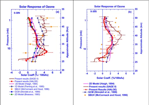
To estimate the seasonal distribution, solar regression coeffi-cients for each month are averaged for all the years. These averaged monthly coefficients are further averaged to obtain an annual regression coefficient at that level. The vertical variation of the annually-averaged solar effect on HALOE and SAGE II ozone over 0–30◦N and 0–30◦S belts are shown in Figs. 2a and b, respectively, along with the one sigma error limit. These results are compared with the so-lar component obtained from the SBUV data (McCormack and Hood, 1996), 2-D model simulations (Brasseur, 1993; Haigh, 1994), 1-D model simulation (Fleming et al., 1995) and a GCM (Shindell et al., 1999). According to our anal-ysis, the solar effect on HALOE and SAGE II ozone is negative near 23 mb (∼26 km) and then positive over the rest of the stratosphere, in both hemispheres and is statis-tically significant for almost all the heights. The magni-tude of the solar coefficient varies with altimagni-tude. Over the 0–30◦N latitudinal belt (Fig. 2a), solar effects on HALOE ozone are negligible at 27 mb (∼25 km), increasing to a max-imum of 4±1.6%/100 sfu by around 10 mb (∼32 km), and declining above that level. It remains almost constant at 2±1.1%/100 sfu in the middle stratosphere and then becomes insignificant near the stratopause. Solar effects on SAGE II ozone exhibit similar variations as those seen in the HALOE
Figure 2 10 1 -4 -2 0 2 4 6 820 25 30 35 40 45 50 55 A p pr ox im a te A lt u tude ( km ) P ressure ( m b)
Solar Coeff. (%/100sfu)
2D Model (Haigh, 1994) Present results (SAGE II) Present Results (HALOE)
Solar Response of Ozone
(b)
GCM (Shindell et al., 1999) SBUV (McCormack and Hood, 1996)
0-30S 10 1 -4 -2 0 2 4 6 8 A p p o xi m ate A ltitu d e ( K m )
Present results (SAGE II) Present results (HALOE)
Solar Response of Ozone
Solar Coeff (% / 100sfu)
0-30N (a) 20 25 30 35 40 45 50 55 Pr essur e ( m b) 2D Model (Haigh, 1994) 1D Model (Fleming et al., 1995) SBUV (McCormack and Hood, 1996) GCM (Shindell.et al., 1999) 2D Model (Brasseur, 1993)
Figure 2
27
Fig. 2. The vertical distribution of annual mean solar coefficient of ozone (%/100 sfu) as obtained in the present study (– HALOE profile)
and (– SAGE II profile) are compared with the results from SBUV data (McCormack and Hood, 1996), indicated by the scatter plot (–), 2-D model (Haigh, 1994) ( -X-), 1-D model (Fleming et al., 1995) (-+), GCM (Shindell et al.,1999) (--), 2-D model (Brasseur, 1993) ( –) over (a) 0–30◦N (b) 0–30◦S latitudinal belts.
profile in the middle stratosphere, except for an additional peak near 2 mb–3 mb. The reason for this peak could be that both HALOE and SAGE II observations are made at a dif-ferent period in a month and the sampling period of these in-struments also differs. This can give rise to tidal error, which amplifies with an increase in altitude. Spatial coverage of these instruments can differ for a month over a selected lati-tudinal belt.
In general, HALOE, SAGE II, 2-D, 1-D models and GCM profiles show similar variations and positive solar responses over 22 mb–0.7 mb (27 km–50 km). In the upper stratosphere of the 0–30◦N belt, 2-D model simulation (Brasseur, 1993; Haigh, 1994) and GCM (Shindell et al., 1999) profiles lie within one sigma error limit of the HALOE profile. In con-trast to HALOE, SAGE II, 2-D, 1-D models and GCM re-sults, SBUV (McCormack and Hood, 1996; Lee and Smith, 2003) and SAGE II (Lee and Smith, 2003) ozone data indi-cate a negative solar effect in the equatorial middle strato-sphere. This apparent negative effect has been attributed to QBO and two major volcanic eruptions, separated by about 9 years. Both eruptions occurred after the solar maximum in the SBUV and SAGE II data periods. The volcanic effect on the solar cycle analysis of ozone variability, using multiple regressions, is expected to be significant. These major vol-canic eruptions enhanced the amount of stratospheric aerosol loading in the equatorial lower stratosphere, which induced intensified upward motion and reduced the equatorial lower
stratospheric ozone for 3-4 years after the eruption (Lee and Smith, 2003). In support of this suggestion, they ran a 2-D model simulation considering the 11-year solar flux variation as only external forcing (without QBO or volcanic effects) and this showed positive peak values in the equatorial upper stratosphere. Study of ozonesonde data from various stations in India shows a solar effect of ∼4–15%/100 sfu over the middle stratosphere, with a maximum near 32 km (Saraf and Beig, 2003). Although the amplitude of the solar effect is much higher than in the present study (which may be due to the specific locations of the ozonesonde observations), the peak near 32 km is consistent with our analysis.
Figure 2b exhibits the vertical profile of the annual mean solar effect on ozone over the 0–30◦S belt. Similar to the 0–30◦N latitudinal belt, the solar effects in the HALOE and SAGE II ozone are negative near 23 mb (26 km) which then increase to a maximum of 4±0.95%/100 sfu near 3 mb (∼40 km) in the SAGE II profile and 2±0.78%/100 sfu near 4 mb (∼38 km) in the HALOE profile, and declines above that level. In general, HALOE and SAGE II profiles show similar variations. Their variabilities are within the one sigma error limit of each other in the middle stratosphere and near stratopause, while a significant difference can be seen only in the upper stratosphere. The maximum differences in their magnitude are observed near 2–3 mb. Similar to the 0– 30◦N belt, the 2-D model (Haigh, 1994) and GCM (Shindell et al., 1999) simulation profiles agree well with the HALOE
2096 S. Fadnavis and G. Beig: Decadal solar effects on temperature and ozone in the tropical stratosphere
(a) (b)
Figure 3
28
Fig. 3. Vertical distribution of the monthly variation of the solar coefficient (%/100 sfu) obtained from the HALOE ozone (a) 0–30◦N (b)
0–30◦S. Monthly variation of 1 sigma error (%/100 sfu) in the solar effect on ozone is over-plotted with thin lines.
profile in the upper stratosphere. In general, the HALOE and SAGEII profiles are in good agreement with the 2-D model and GCM simulations but not with the SBUV results.
The HALOE and SAGE II profiles show similar variations in the respective belts. These profiles show good agreement in the middle stratosphere (they lie within the error bars of each other) while they differ in the upper stratosphere. So-lar signals in the HALOE and SAGE II ozone show a peak in both the 0–30◦N and 0–30◦S belts at different altitudes. The HALOE profile exhibits a peak near 10 mb (32 km) in the Northern Hemisphere and rear ∼4 mb (38 km) in the South-ern Hemisphere. Over the 0–30◦N belt, the solar response in the SAGE II ozone shows two maxima, one near 10 -mb (similar to HALOE) and another near the 3 -mb level. In the Southern Hemisphere it shows only one peak near the 3 -mb pressure level. Interestingly, the maximum solar effect on ozone (HALOE and SAGE II) near 10 mb in the North-ern Hemispheric belt and near 7 mb–4 mb in the SouthNorth-ern Hemispheric belt, as observed in the present analysis, have not been reported previously. This aspect is related to the seasonal distributions of the solar effect on ozone (see Dis-cussion section).
Figures 3a and b show the monthly variation of the solar effect on ozone (%/100 sfu), as obtained from HALOE, over 0–30◦N and 0–30◦S, respectively, for the 27 mb–0.8 mb
pressure levels (∼25 km–50 km). The corresponding one
sigma error limit is over-plotted with thin lines. Over both the northern and southern belts, a positive solar coefficient of ∼2–6%/100 sfu is observed in most of the stratospheric
region, with a pocket of negative coefficients during March and September near 27 mb (∼25 km). In the middle strato-sphere, not much seasonal variation is seen, consistent with the results of Brasseur (1993) over the tropics. In the 18 mb– 9 mb (∼28 km–33 km) region, a strong, positive solar coeffi-cient with values greater than 6%/100 sfu are observed dur-ing the months of January, February and March, in the North-ern Hemisphere. Similar high values are observed during these months but at higher altitudes (∼8 mb) in the Southern Hemisphere. The effect of these high positive values can be seen as a peak in the annual mean profile. Oscillation of a 3–5 month periodicity is observed above 2 mb in both hemi-spheres.
Figures 4a and b show monthly distributions of the solar effect on SAGE II ozone over 0–30◦N and 0–30◦S belts, re-spectively. The corresponding one sigma error limit is over-plotted with thin lines. A strong positive solar coefficient with values greater than 6%/100 sfu is observed near 10 mb during January, February and March over the 0–30◦N belt, which is observed at higher altitudes (∼4 mb) in the South-ern Hemisphere. Such a strong, positive solar coefficient is also observed in the solar effects on the HALOE ozone over similar pressure levels of respective latitudinal belts. The monthly distribution of solar effects on SAGE II ozone is quite similar to that of the HALOE ozone over the 0–30◦S belt while their structure differs over the 0–30◦N belt. Os-cillation of a 3–5 month periodicity is observed above 2 mb in both hemispheres.
(a) (b)
Figure 4
29
Fig. 4. Vertical distribution of monthly variation of solar coefficient (%/100 sfu) obtained from SAGE II ozone (a) 0–30◦N (b) 0–30◦S.
Monthly variation of 1 sigma error (%/100 sfu) in the solar effect on ozone is over-plotted with thin lines.
3.2 Solar effect on temperature
The vertical variations of the annual mean solar regression coefficient, δ(z), deduced from HALOE and SAGE II tem-peratures over the 0–30◦N and 0–30◦S belts, are shown in Figs. 5a and b, respectively, with a one sigma error limit. Figure 5 also shows the results obtained by Rocketsonde and SSU/MSU temperature (Keckhut et al., 2005), National Me-teorological Center (NMC) temperature (McCormack and Hood, 1996), SBUV (McCormack and Hood, 1996), 2-D model simulations (Brasseur, 1993 and Haigh, 1994), and one-dimensional Fixed Dynamical Heating (FDH) ra-diative model simulations (McCormack and Hood, 1996). Figure 5a shows that the solar coefficient obtained from the HALOE temperature is found to be significant in the lower (below 18 mb that is below 28 km) and upper strato-sphere (above 2 mb that is above ∼43 km), but it is insignif-icant in the mid-stratosphere over the 0–30◦N belt. Over the 0–30◦S belt the HALOE profile shows similar varia-tions but it is significant almost throughout the stratosphere. Over both belts the solar response in HALOE temperature is found to be highest (∼1.1±0.23 K/100 sfu) at about 27 mb (∼25 km). This starts decreasing and becomes negligible
between 7 mb–2 mb (35 km–43 km). Above 2 mb (above
43 km), it again increases with height and reaches a value of ∼0.7±0.3 K/100 sfu near the stratopause. The minimum solar response in the HALOE temperature is more prominent in the Southern Hemisphere as compared to that in the
North-ern Hemisphere. The vertical profile of the solar coefficients obtained from the SAGE II temperature shows similar varia-tions as that of the HALOE profile over the respective belts, except for a minimum solar response near 5 mb (37 km) in-stead of 10 mb (32 km). In both 0–30◦N and 0–30◦S belts the HALOE and SAGE II profiles lie within the one sigma er-ror limit of each other, except in the region of minimum solar response. The variation of the HALOE and SAGE II vertical profiles, as obtained in present study, are broadly consistent with the NMC (in the Northern Hemisphere) and the SBUV (in both hemispheres ) observational results in the middle stratosphere. The derived solar effects in the HALOE and SAGE II temperatures are smaller than the 2-D, FDH and SBUV results in the upper stratosphere and the SSU/MSU results (Keckhut et al., 2005) in the middle stratosphere over both hemispheres. The differences in the magnitudes of so-lar coefficients obtained by different workers could be due to the difference in the latitudinal region considered in each study. The 2-D results by Brasseur (1993) are at 5◦N, the 2-D results by Haigh (1994) are over 0–30◦S, the SSU/MSU results are over the sub-tropics and the NMC results are over the entire globe. What is worth noting is that the shape of the vertical profiles is largely consistent with the results ob-tained here. Present results indicate (over both hemispheres) a minimum solar coefficient around 10 mb, (∼32 km) in the HALOE profile and 5 mb (∼37 km) in the SAGE II temper-ature profile, where the coefficient becomes negative. It is insignificant in the HALOE and SAGE II profiles over the
2098 S. Fadnavis and G. Beig: Decadal solar effects on temperature and ozone in the tropical stratosphere 10 1 -2 -1 0 1 2 3 4 A pproxim ate A ltit u d e (km )
Solar Response of Temperature
P
res
sure (
m
b)
Solar Coeff. (K/100sfu)
0-30N (a) 20 25 30 35 40 45 50 55
Present results (HALOE) 2D Model (Haigh, 1994) SBUV (McCormack and Hood, 1996) Present results (SAGE II) SSU/MSU (Keckhut et al., 2005) Rocksonde (Keckhut et al., 2005) NMC (McCormack and Hood, 1996) 2D model (Brasseur, 1993) FDH Model (McCormack and Hood, 1996)
10 1 -2 -1 0 1 2 3 4 20 25 30 35 40 45 50 55 Pr essur e ( m b ) A p p ro xim at e A lt itu te (k m )
Solar Coeff (K/100sfu)
SSU/MSU (Keckhut et al., 2005) 2D Model (Haigh, 1994) Present results (SAGE II ) Present results (HALOE)
0-30S
Solar Response of Temperature (b)
SBUV (McCormack and Hood, 1996) FDH Model (McCormack and Hood, 1996)
Figure 5
30
Fig. 5. The vertical distribution of the annual mean solar coefficient of temperature (K/100 sfu) as obtained in the present study (– HALOE
profile) and (– SAGE II profile) are compared with Rocketsonde (Keckhut et al., 2005) (-♦-), SSU/MSU (Keckhut et al., 2005) (-+-), NMC results (McCormack and Hood, 1996) (–), FDH model results (McCormack and Hood, 1996) (-*-), 2-D model results (Brasseur, 1993) (–) and 2-D model results (Haigh, 1994) (– ) over (a) 0–30◦N (b) 0–30◦S latitudinal belts.
0–30◦N belt. It is significant in the SAGE II profile and in-significant in the HALOE profile over the 0–30◦S belt. The change in temperature from NCEP to the HALOE CO2 chan-nel, near 5 mb (∼37 km), may affect these altitudes. This may be the reason why the HALOE profile shows solar min-imum at a different pressure level than that of the SAGE II profile. A negative solar response is also evident in the SBUV, NMC and FDH model profiles, as shown in Fig. 5. Such negative solar response is also observed over north-ern latitudes in satellite derived profiles (Ramaswamy et al., 2001), in the OHP lidar record (Keckhut et al., 1995) and in a rocket record (Kokin et al., 1990) near 30 km. Balachan-dran and Rind (1995) reported that this alternation of the sign of the solar signal could be due to a dynamical effect. Con-sistent with the present results, Hood (2004) found a positive temperature response maximizing at the stratopause. Later, it decreases to 0 K and –1 K at 34 km and 32 km, respectively.
Model simulations by Huang and Brasseur (1993) found less than a 1.5-K increase in temperature due to an increase in solar activity associated with the 11-year solar cycle. At mid stratospheric levels, 13 mb–3 mb (30 km–40 km), the ob-served variability (in HALOE SAGE II SBUV and NMC) is less than the model predictions. From the HALOE temper-ature, the solar coefficient derived by Remsberg and Deaver (2005) varies from 0.72 K to 1.18 K over tropics (10◦wide belts) in the upper stratosphere (35 km–50 km). Solar coef-ficients obtained in the present study are smaller than those
reported in Remsberg and Deaver (2005). This could be due to an averaging of responses in the temperature profiles over the entire tropical belt. From the ERA-40 data set for the period 1979–2001, Crooks and Gray (2005) found a pos-itive solar effect throughout the tropical stratosphere, with an amplitude of 1.75 K, peaking at 43 km. In the middle stratosphere solar coefficients were observed to vary from 0.18 to 0.81 K/100 sfu over different Indian stations (Saraf and Beig, 2003). Using radiosonde and rocketsonde data, Angell (1991) estimated a solar cycle variation of approx-imately 0.2 K–0.8 K, from the lower to upper stratosphere. The overlap-adjusted SSU plus MSU data sets deduce a so-lar component of the order of 0.5 K to 1.0 K throughout the low-latitude stratosphere (Hood and Soukharev, 2001). Ra-maswamy et al. (2001) reported a solar signal of ∼0.5 K– 1.0 K in the Nash (SSU 15X) satellite data. These results are broadly in agreement with ours.
Monthly variations in the vertical profile of the solar coef-ficient in the HALOE temperature over 0–30◦N and 0–30◦S are plotted in Figs. 6a and b, respectively; the corresponding one sigma error limit is over-plotted with thin lines. The most obvious feature is that both the 0–30◦N and 0–30◦S belts ex-hibit strong, negative solar response (<–2 K/100 sfu) during August–October between 15 mb–3 mb, with a minimum am-plitude near 10 mb (∼32 km). The solar response over the 0–30◦N belt shows another minimum near 4 mb (∼38 km). A negative solar response, although insignificant, persists
(a)
(b)
Figure 6
31
Fig. 6. Vertical distribution of the monthly variation of the solar coefficient (K/100 sfu) obtained from HALOE temperature (a) 0–30◦N (b)
0–30◦S. Monthly variation of 1 sigma error in the solar effect on temperature is over-plotted with thin lines.
(a) (b)
Figure 7
Fig. 7. Vertical distribution of monthly variation of solar coefficient (K/100 sfu) obtained from SAGE II temperature (a) 0–30◦N (b) 0–30◦S.
Monthly variation of 1 sigma error (K/100 sfu) in the solar effect on temperature is over-plotted with thin lines.
2100 S. Fadnavis and G. Beig: Decadal solar effects on temperature and ozone in the tropical stratosphere until March in the Northern Hemisphere and throughout the
year in the Southern Hemisphere. Cyclic variation with 3– 5 month periodicity is evident above 2 mb (∼43 km) in the northern belt. This is also observed in the SAGE II tempera-ture over the 0–30◦N belt.
Figures 7a and b exhibit the monthly variation of so-lar coefficients for the SAGE II temperature over 0–30◦N and 0–30◦S, with one sigma error limit over-plotted with thin lines. Similar to the HALOE temperature strong, neg-ative coefficients (<–2 K/100 sfu) are also observed during August-October near 15 mb–3 mb with a minimum near 5 mb (∼37 km) over northern and southern belts. These negative coefficients persist until February in both the hemispheres. In the Northern Hemisphere cyclic variation of 3–5 months, periodicity is observed near the stratopause. In general, pos-itive responses are found for almost all months except for August–March at some pressure levels. These dips in tem-perature, are also reflected in the annual mean profile, which could be due to the dynamical effect.
If we compare monthly mean variations of solar response in temperature deduced from HALOE and SAGE II instru-ments over the Northern Hemisphere, the prominent com-mon features are the dips in temperature near 4 mb–5 mb during August to October and the 3–5 months cyclic vari-ations near the stratopause. Their structure over rest of the stratosphere differs. The probable reasons may be that ob-servations are made at different periods in the month, or in the sampling periods these instruments also differ, or differ-ent latitudinal coverage occurs for a month within the belt. Similarly, over the 0–30◦S belt common features of the solar signal in the HALOE and SAGE II temperature shows good agreement.
4 Discussion
Annual mean solar responses on HALOE and SAGE II ozone are in good agreement in the middle stratosphere. However, they differ in the upper stratosphere. The reasons for this disagreement could be that their observations are made at different periods in the month, and the sampling period of these instruments differs, which may give rise to tidal error. Tidal interference amplifies at higher altitude. Another rea-son could be their different latitudinal coverage in a month within the selected belt.
Annual mean solar response in the HALOE and SAGE II temperatures are in good agreement through out the strato-sphere. In the upper stratosphere the solar response on HALOE and SAGE II ozone exhibits a disagreement, whereas their solar responses in temperature are in good agreement. The reason for the agreement in the upper strato-sphere could be due to the inclusion of NCEP estimates above 5 mb in the HALOE temperature profiles, which re-duces the effect of tidal interferences.
Monthly mean variation of solar responses in ozone and temperature obtained from respective instruments show a similarity in prominent features over both hemispheres. Both HALOE and SAGE II ozone show an enhanced so-lar response near 10 mb (∼32 km) in the Northern Hemi-sphere, and ∼–7 mb–4 mb in the Southern Hemisphere dur-ing January–March (winter and beginndur-ing of sprdur-ing). In both hemispheres, HALOE and SAGE II temperatures show a negative solar response from August to February while keep-ing the strong amplitude durkeep-ing August–October (late sum-mer and early autumn) at 10 mb and at 5 mb, respectively. It is interesting to note that over both hemispheres, the so-lar response in temperature shows a dip (10 mb HALOE and 5 mb in SAGE II) during August to October (autumn) while the solar response in ozone shows an enhancement during the following season (winter) at similar altitudes.
The cyclic variation of 3–5 months periodicity is quite prominent in the altitudes above 2 mb in the HALOE and SAGE II ozone over both belts, while in the solar response to temperature 3–5 month periodic variations can be seen in the SAGE II and HALOE only in the Northern Hemisphere. It is evident from Figs. 3 and 6 that the solar response of the HALOE ozone is out of phase with the HALOE temper-ature in the upper stratosphere. However, they are in phase in the middle stratosphere (between 27 mb and 18 mb). A similar phase relationship is also observed in the SAGE II ozone and temperature (Figs. 4 and 7). Saraf and Beig (2003) also reported a significant in phase relation between the so-lar component of the temperature and ozone in the middle stratosphere over different Indian stations, which is reason-ably in agreement with the present results. The correlation between the solar component of the ozone and the solar com-ponent of the temperature shows a positive correlation in the middle stratosphere and a negative correlation in the upper stratosphere. The reason may be that since the majority of the apparent solar cycle variation of ozone takes place in the lower stratosphere (Hood, 1997; Wang et al., 1996), ozone increases from solar minimum to solar maximum. This in-crease in ozone will lead to an inin-crease in UV absorption and therefore in temperature. Temperature also increases from solar minimum to solar maximum. Hence, the solar compo-nent of the ozone is positively correlated to the solar response of the temperature in the lower and middle stratosphere. In the upper stratosphere the solar response of the ozone to the solar cycle takes place through a temperature dependence of reactions (1) O+O3→2O2, (2) O+O2+M→O3+M. The tem-perature increases from solar minimum to solar maximum. Ozone changes are anti-correlated to the temperature varia-tions due to the inverse dependence of the above photochem-ical reaction rates of ozone on temperature (Saraf and Beig, 2003). Therefore, the solar component of the ozone and so-lar component of temperature are anti-correlated in the up-per stratosphere, which is highest near the stratopause where temperature variation due to solar flux is also high.
Our statistical analysis of the annual mean response of HALOE ozone (over 0–30◦N and 0–30◦S belts) to the 11-year solar cycle matches reasonably with the 2-D model and the GCM profiles, as compared to SAGE II ozone profile. The agreement between the solar responses in the HALOE ozone to the model simulated results is particularly good over the upper stratosphere compared to the middle stratosphere. The solar response on the upper stratospheric SAGE II ozone agrees qualitatively with the HALOE and model simulated results. The reasons for this agreement, especially over the 3 mb–0.8 mb (∼40 lm–50 km) pressure levels, could be that at these levels ozone is nearly in a state of photochemical equilibrium, where transport effects are less important, and ozone photochemistry is accurately simulated by these mod-els. The annual solar effect on ozone obtained in the present study is stronger near 10 mb (∼32 km) and ∼3 mb (∼40 km) than that predicted by models. This discrepancy in this re-gion could be due to less penetration of UV radiation in the Herzberg continuum (200 nm–240 nm) caused by greater ab-sorption at higher altitudes. Therefore, ozone becomes less sensitive to photochemistry (Brasseur and Simon, 1990) and the distribution of ozone is controlled primarily by dynam-ics (McCormack and Hood, 1996). Dynamical phenomenon may be responsible for the observed peak.
The annually averaged solar effect on temperature ob-tained in the present study (SAGE II and HALOE, over 30◦N and 0–30◦S belts) is stronger near 27 mb (25 km) and weaker in the upper stratosphere, as compared to model results. In contrast to model results, a weak (statistically insignifi-cant), negative solar effect is observed near 10 mb (∼32 km) in HALOE and 5 mb (∼37 km) in SAGE II. Monthly dis-tributions of solar effects on temperature reveal that this negative response takes place during August to March, be-tween 18 mb–3 mb (28 km–40 km), with a minimum dur-ing August–October near 10 mb in HALOE and near 5 mb (∼37 km) in SAGE II.
As noted above, our analysis finds that a feature in the annually averaged solar effect on ozone at 10 mb (0–30◦N) and 3 mb (0–30◦S) is much stronger than predicted in the models. On a monthly basis, a strong, positive response is observed during January–March. Over the same pressure levels, the annual mean solar effect on temperature becomes negative at 10 mb in HALOE and 5 mb (∼37 km) in SAGE II temperature profiles. The change over of temperature from
NCEP to the HALOE CO2 channel near 5 mb may affect
these pressure levels and this may be the reason for an ob-served negative minimum near 10 mb instead of 5 mb. The monthly variation reveals that this strong, negative response takes place during August-March with a minimum amplitude during August-October, when the solar effect on temperature becomes negative with a strong amplitude during autumn and in the following season (winter) the solar effect on ozone shows an enhancement over the same pressure levels. This indicates that the dynamical phenomena may be affecting the solar signal at these altitudes. Because of the limited duration
of data recorded (13 years), the regression analysis used may not isolate the true signal in response to the 11-year solar cy-cle from other nonlinear geophysical forcing, such a QBO. Longer observational data records, at least for 2–3 decades, are necessary to isolate the effect of the solar cycle precisely.
5 Conclusions
The HALOE and SAGE II temperature and ozone measure-ments are used for the investigation of the 11-year solar sig-nal. Our analysis of this effect demonstrates a positive an-nual response in temperature and ozone over both belts (0– 30◦N and 0–30◦S). The annually averaged signal in ozone (HALOE and SAGE II) is found to be of the order of around 1±0.5 to 4±1.6%/100 sfu and highly significant in most of the stratospheric regions. The deduced solar response of the HALOE ozone is in a general agreement with the SAGE II ozone. Over the 0–30◦N belt the solar signal in the HALOE ozone exhibits a pronounced peak near 10 mb (∼32 km) and in the SAGE II ozone it shows an enhance-ment near 10 mb (∼32 km) and 3 mb (∼40 km). In the South-ern Hemisphere solar signals in the HALOE and SAGE II ozone show an enhancement near 3 mb. The solar response in the HALOE ozone shows a very good agreement with the model simulated results in the upper stratosphere. A solar effect of 0.4±0.23 to 0.8±0.46 K/100 sfu is observed in the lower and upper stratospheric temperature (HALOE and SAGE II), with a negative response in the middle strato-sphere. Annual mean solar signals deduced from HALOE and SAGE II temperature are in good agreement throughout the stratosphere. Annual solar response in temperature shows a dip near 10 mb (∼32 km) in the HALOE profile and 5 mb (∼43 km) in SAGE II profile. The solar effect on temperature indicates a negative response during August-March, with a minimum during autumn, while the solar effect on ozone in-dicates a high positive solar effect in the middle stratosphere during following season (winter). This dip in the tempera-ture effect and peak in the ozone effect may be attributed to a dynamical phenomenon. More detailed investigation of this possibility is needed. The solar signal in ozone shows an in-phase relationship with temperature in the middle strato-sphere. They are out of phase in the upper stratostrato-sphere.
Acknowledgements. The authors express gratitude to G. B. Pant
(IITM) for his encouragement during the course of this study. Thanks are due to T. Anderson and R. Saylor for their valuable help in language editing. We are also grateful to two anonymous reviewers. We acknowledge the Climate and Weather of Sun Earth System–India (CAWSES) program of Indian Space Research Orga-nization for the financial assistance to this project.
Topical Editor U.-P. Hoppe thanks two referees for their help in evaluating this paper.
2102 S. Fadnavis and G. Beig: Decadal solar effects on temperature and ozone in the tropical stratosphere References
Angell, J. K.: Stratospheric temperature change as a function of height and sunspot number during 1972–1989 based on rocket-sonde and radiorocket-sonde data, J. Climate, 4, 1170–1180, 1991. Angell, J. K.: On the relation between atmospheric ozone and
sunspot number J. Clim., 2, 1404–1416, 1989.
Balachandran, N. K. and Rind, D.: Modeling the effects of UV variability and the QBO on the troposphere system, I, The middle atmosphere, J. Clim., 8, 23 079–23 090, 1995.
Brasseur, G.: The response of the middle atmosphere to long term and short term solar variability: A two-dimensional model, J. Geophys. Res., 98, 23 079–23 090, 1993.
Brasseur, G. A., Rudder, De, Keating, G. M., and Pitts, M. C.: Re-sponse of middle atmosphere to short term solar ultraviolet vari-ations, 2 Theory, J. Geophys. Res., 92, 903–914, 1987.
Brasseur, G. and Simon, P. C.: Stratospheric Chemical and ther-mal response of middle atmosphere to short-term solar ultraviolet variations, 2, Theory, J. Geophys, Res., 95, 5639–5655, 1990. Callis, L. B. and Nealy, J. E.: Solar UV variability and its effect on
stratospheric thermal structure and trace constituents, Geophys. Res. Lett., 5, 249–252, 1987.
Chandra, S. and McPeters, R. D.: The solar cycle variation of ozone in the stratosphere inferred from Nimbus 7 and NOAA 11 satel-lites, J. Geophys. Res., 99, 20 665–20 671, 1994.
Crooks, S. A. and Gray, L. J.: Characterization of the 11 year so-lar signal using a multiple regression analysis of the ERA-40 Dataset, J. of Clim., 18, 996–1015, 2005.
Cunnold, D. M., Chu, W. P., Barnes, R. A., McCormick, M. P., and Veiga, R. E.: Validation of SAGE II ozone measurements, J. Geophys. Res., 94, 8447–8460, 1989.
Dunkerton, T. J., Delisi, D. P., and Baldwin, M. P.: Middle at-mosphere cooling trend in historical rocketsonde data, Geophys. Res. Lett., 25, 3371–3374, 1998.
Fleming, E., Chandra, S., Jackman, C. H., Considine, D. B., and Douglass, A. R.: The middle atmosphere response to short and long term solar UV variation: Analysis of observations and two dimensional model results. J. Atmos. Terr. Phys., 57, 333–365, 1995.
Haigh, J. D.: A GCM study of climate change in response to 11 year solar cycle , Q. J. R., Meteoro, Soc., 125, 871–892, 1999. Haigh, J. D.: The impact of solar variability on climate, Science,
272, 981–984, 1996.
Haigh, J. D.: The role of stratospheric ozone in modulating the solar radiative forcing of climate, Nature, 370, 544–546, 1994. Hood, L. L.: Effects of solar UV variability on the stratosphere,
in: Solar variability and its effect on the Earth’s atmosphere and climate system, AGU Monograph Series, edited by: Pap, J. and Fox, P., American Geophysical Union, Washington D.C., Vol. 141, 283–303, 2004.
Hood, L. L. and Soukharev, B. E.: The solar component of long-term stratospheric variability: observations, model comparisons and possible mechanisms, Proceedings of the SPARC 2000 Meeting, Mar del Plata, Argentina, O.2/14.available on CDROM, 2001.
Hood, L. L.: The solar cycle variations of total ozone: Dynamical forcing in the lower stratosphere, J. Geophys. Res., 102, 1355– 1370, 1997.
Hood, L. L. and Jirikowic, J., and McCormack, J. P.: Quasi-decadal variability of the stratosphere: Influence of long term solar
ultra-violet variations, J. Atmos. Sci., 50, 3941–3958, 1993.
Hood L. L.: Coupled stratospheric ozone and temperature response to short term changes in solar ultraviolet flux: An analysis of Nimbus 7 SBUV and SAMS data, J. Geophys. Res., 91, 5264– 5276, 1986.
Huang, T. Y. W. and Brasseur, G.: Effect of long-Term Solar Vari-ability in a Two-Dimensional Interactive Model of the Middle Atmosphere, J. Geophys. Res., 98, 20 413–20 427, 1993. Jackman, C. H., Fleming, E. L., Chandra, S., Considine, B. D.,
and Rosenfield, J. E.: Past, present and future modeled ozone trends with comparisons to observed trends, J, Geophys. Res., 101, 28 753–28 767, 1996.
Keckhut, P., Cagnazzo, C., Chanin, M. L., et al.: The 11-year solar-cycle effects on the temperature in the upper-stratosphere and mesosphere: Part I-Assessment of Observations, J. Atmos. Sol. Terres. Phys., 67, 948–958, 2005.
Ketchut, P., Hauchecorne, A., and Chanin, M. L.: Midlatitude long-term variability of the middle atmosphere: Trends and cyclic and episodic changes, J. Geophys. Res., 100, 18 887–18 897, 1995. Kokin, G., Lysenko, Y., and Rozenfeld, S.: Temperature changes in
the stratosphere and mesosphere in 1964–1988 based on rocket-sonde data, Izv. Atmos. Oceanic Phys., 26(6), 518–523, 1990. Labitzke, K., Austin, J., Butchart, A., Knight, J., Takahashi, M.,
Nakamoto, M., Nagashima, T., Haigh, J., and Williams, V.: The global signal of the 11-year solar cycle in the stratosphere: Ob-servations and models, J. Atmos. and Solar Terr. Phy., 64, 203– 210, 2002.
Labitzke, K.: The Global signal of the 11 year sunspot cycle in the stratosphere: Differences between solar maxima and minima, Meteorologische Zeitschrift, 10, 83–90, 2001.
Lee, H. and Smith, A.: Simulation of the combined effects of solar cycle, QBO, and volcanic forcing on stratospheric ozone changes in recent decades, J. Geophys. Res., 108(D2), 4049, doi:10.1029/2001JD001503, 2003.
Loon, H. van and Labitzke, K.:The signal of the 11-yearsolar cycle in the global stratosphere, J. Atmos. and Solar Terr. Phy., 61, 53– 61, 1999.
McCormack, J. P. and Hood, L. L.: Apparent solar cycle variations of upper stratospheric ozone and temperature: Latitudinal and seasonal dependences, J. Geophys. Res., 101, 20 933–20 944, 1996.
Miller, A. J., Nagatani, R. M., Tiao, G. C., Niu, X. F., Reinsel, G. C., Wuebbles, D., and Grant, K.: Comparison of observed ozone and temperature trends in the lower stratosphere, Geophys. Res. Lett., 19, 929–932, 1992.
Ramaswamy, V., Chanin, M. L., Angell, J., et al.: Stratospheric temperature trends: Observations and model simulations, Rev. Geophys., 39, 71–122, 2001.
Randel, W. J., Stolarski, R. S., Cunnold, D. M., Logan, J. A., Newchurch, M. J., and Zawodny, J. M.: Trends in the Vertical Distribution of Ozone, Science, 285, 1689–1692, 1999. Randel, W. J. and Cobb, J. B.: Coherent variations of monthly
mean total ozone and lower stratospheric temperature, J. Geo-phys. Res., 99, 5433–5477, 1994.
Remsberg, E. E. and Deaver, L. E.: Interannual Solar cy-cle, and trend terms in middle atmospheric temperature time series from HALOE. J. Geophys. Res., 110, D06106, doi:10.1029/2004JD004905, 2005.
Remsberg, E. E., Bhat, P. P., and Deaver, L. E.: Seasonal
and long-term variations in middle atmosphere temperature from HALOE on UARS, J. Geophys. Res., 107, D19, 4411, doi:10.1029/2001JD001366, 2002.
Rind, D. P., Lonergan N. K., Balachandran, N., and Shindell, D.: 2xCO2and solar variability influences on troposphere through
wave mean flow interaction, J. Meteorol Soc., Jpn., 80, 863–976, 2002.
Saraf, N. and Beig, G.: Solar Response in the Vertical Structure of Ozone and Temperature in the Tropical Strato-sphere, J. Atmos. Solar Terr. Phys., 65(11–13), 1235–1243, doi:10.1016/j.jastp.2003.08.006, 2003.
Shindell, D., Rind, D., Balachandran, N., Lean, J., and Lonergan, J.: Solar cycle variability, Ozone and climate, science, 284, 305– 308, 1999.
Stolarski, R. S., Bloomfield, P., McPeters, R. D., and Herman, J. R.: Total ozone trends deduced from Nimbus 7 TOMS data, Geo-phys. Res. Lett., 18, 1015–1018, 1991.
Wang, H. J., Cunnold, D. M., and Bao, X.: A critical analysis of stratospheric aerosol and gas experiment ozone trends. J. Geo-phys. Res., 101, 12 495–12 514, 1996.
Wuebbles, D. J., Kinnison, D. E., Grant, K. E., and Lean, J.: The effect of solar flux variations and trance gas emissions on re-cent trends in stratospheric ozone and temperatutre, J. Geomagn. Geoelect., 43, 709–718, 1991.
Zerefos, C. S., Tourpali, K., Bojkov, B. R., and Balis, D. S.: So-lar activity-total column ozone relationships: Observations and model studies with heterogeneous chemistry, J. Geophys. Res., 102, 1561–1569, 1997.