Reliability analysis of bonded joints with variations in adhesive thickness

HAL Id: hal-00920724

https://hal.archives-ouvertes.fr/hal-00920724

Submitted on 28 Jan 2014

HAL is a multi-disciplinary open access

archive for the deposit and dissemination of sci-entific research documents, whether they are pub-lished or not. The documents may come from teaching and research institutions in France or abroad, or from public or private research centers.

L’archive ouverte pluridisciplinaire HAL, est destinée au dépôt et à la diffusion de documents scientifiques de niveau recherche, publiés ou non, émanant des établissements d’enseignement et de recherche français ou étrangers, des laboratoires publics ou privés.

Jean-Denis Mathias, M. Lemaire

To cite this version:

Jean-Denis Mathias, M. Lemaire. Reliability analysis of bonded joints with variations in adhesive thickness. Journal of Adhesion Science and Technology, Taylor & Francis, 2013, 27 (10), p. 1069 - p. 1079. �10.1080/01694243.2012.727176�. �hal-00920724�

Reliability Analysis of Bonded Joints with Variations in Adhesive Thickness

Jean-Denis MATHIAS*

IRSTEA,

Laboratoire d’Ingénierie pour les Systèmes Complexes,

Campus des Cézeaux, 24 Avenue des Landais – BP 50085, 63172 Aubière Cedex, France

Maurice LEMAIRE

Clermont Université, Institut Français de Mécanique Avancée, EA 3867,Laboratoire de Mécanique et Ingénieries,

Campus de Clermont-Ferrand les Cézeaux - BP265, 63175 AUBIERE Cedex, France

Short Title: Reliability analysis of bonded joint

*Corresponding author: email:[email protected], tel: +33(0)473440680, fax :

ABSTRACT

Bonded joints are used in several industrial applications as a surrogate of more expensive repairs, but their reliability must be ascertained. Failure in a bonded joint mainly occurs in the adhesive due to stress concentrations that directly depend on the adhesive thickness. In practice, it is difficult to ensure a good accuracy of the final adhesive thickness, leading to uncertainty to its spatial variability. This uncertainty greatly influences the strength of the bonded joint. This work deals with one of the main key-issues in bonded joints: the influence of the spatial variations in the adhesive thickness on the reliability of the joint; an excessive shear stress level caused by the adhesive thickness variations may lead to failure. This paper provides reliability analysis by considering the adhesive thickness as a stochastic field. The experimental thickness field is obtained so as to identify the stochastic parameters. These parameters are then introduced in a structural reliability model to evaluate the failure probability. Results show the influence of adhesive thickness uncertainty on bonded joint failure.

KEYWORDS: bonded joint, failure, shear stress, adhesive thickness, stochastic field,

1 Introduction

Bonded composite patches are used as structural repairs in several fields such as civil engineering for damaged concrete structures [1] or aeronautics for components which exhibit damages, defects or impacts [2]. Another industrial application consists in using patches for the prevention of damage appearance. The service life of such reinforced structures is expected to be increased and expensive repairs or replacements are also expected to be avoided. However, it is well known that shear stress peaks near the free edges of the composite patches may cause failure of the joint. Indeed, some studies have shown that 53% of significant defects on bonded structures proceed from adhesive bond failures [3].

The shear-lag model was the first model which enabled the calculation of stress distribution in the adhesive, and consequently the prediction of bonded joint failure [4]. This model was then refined to account for some additional factors such as spew fillet [5], large deflections [6] or possible elastic–plastic response of the adhesive [7,8]. Some other non-linear models have been developed, for instance to take into account the viscoelasticity of the adhesive [9] or the influence of the load level on the parameters of the Burgers model [10]. It is well known that the adhesive thickness greatly influences the shear stress distribution. Several studies have shown the influence of this parameter. For example, cohesive zone models have been used to analyze the influence of the adhesive thickness [11]. A comparative numerical and experimental study has also been done for aluminum single-lap joints bonded with aluminum powder filled epoxy adhesive [12]. The type of failure according to the adhesive thickness has been also studied [13].

It is commonly admitted that adhesive thickness presents some uncertain variations owing to the joint fabrication process. These variations can significantly increase the shear stress peak near the free edge of the joint. Reliability methods [14] can take into account this variability by considering the adhesive thickness as a stochastic field. Therefore, it enables the assessment of the failure probability of the bonded joint. Linear or quadratic approximations of the limit state (characterizing the bonded joint failure) or response surface approximations can be used for the calculation of this failure probability avoiding a too high number of simulations such as classical Monte Carlo simulations [14] [15]. It has been successfully applied in several studies, especially in mechanical applications [16] [17].

An experimental investigation of adhesive thickness variations is first addressed in this paper. For this purpose, a three-dimensional measuring machine is used in order to obtain the adhesive thickness field of bonded joint. The stochastic parameters of the adhesive thickness field are then identified by a stochastic decomposition. Afterwards, these parameters are introduced in a structural reliability model to calculate failure probabilities and normalized sensitivities with respect to the mean [14]. Finally, the reliability model is used to calculate the safety coefficient for a target failure probability.

2. Experimental assessment of the adhesive 2.1 Experimental set-up

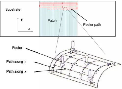
Single-lap specimens have been prepared by the industrial partner, “AIA of Clermont-Ferrand” (French Ministry of Defence). Composite patches were bonded to aluminium (see Figure 1). The substrate was made of aluminium 2024 T3 with a thickness 4 mm. The composite patch was made of Hexcel carbon prepreg system 914 T300 (epoxy/carbon). Four

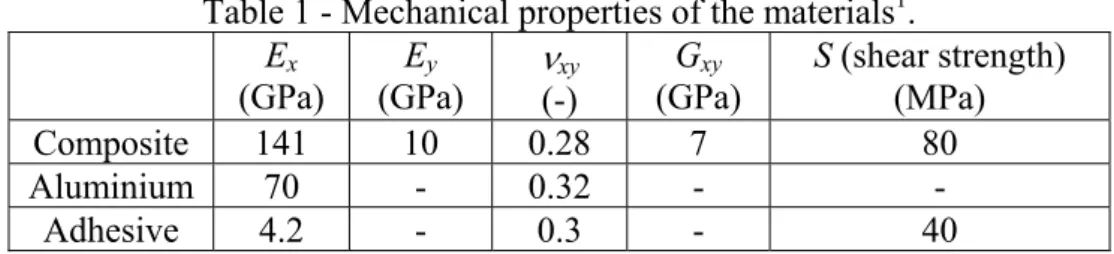
unidirectional plies were used. The total thickness of the patch was 0.5 mm. The dimensions of the composite patch were equal to LxL with L=70 mm. The adhesive used was a Redux 312 adhesive. The initial setting of the adhesive thickness during the joint fabrication process was 0.15 mm. Mechanical properties of each material are reported in Table 1.

As mentioned above, the adhesive thickness may present some uncertain variations owing to the joint fabrication process. Before identifying the stochastic parameters, the adhesive thickness field has to be measured. For this purpose, a three-dimensional measuring machine (MMT TEMPO MCA 10 from TRI-MESURES, France) was used here to obtain the thickness field of the adhesive with respect to the x- and y-directions. The resolution was 5 µm. Measurements were made on both faces of the specimen. The pitch u (the distance between two measures) here was 1.1 mm which corresponds to 64 pitches for the specimen length in the x-direction. 37 pitches were used for the specimen width in the y-direction. The path of the feeler of the three-dimensional measuring machine is represented in Figure 1. The total thickness ttot(x,y) was then obtained. The composite thickness tcomp(x,y) and the aluminium thickness talu(x,y) were assumed to be constant. The adhesive thickness tadh(x,y) can be determined as follows:

) , ( ) , ( ) , ( ) , (x y t x y -t x y -t x y

tadh _ tot alu comp ₍₁₎

Note that variations in thicknesses of the aluminium plate talu(x,y) and of the composite

tcomp(x,y) were negligible in comparison with the adhesive thickness variations.

2.2 Field decomposition

The adhesive thickness tadh(x,y) is now considered as a stochastic field tadh(x,y,ω) in which are random points in space . In the following, we consider a one-dimensional mechanical model based on the Volkersen’s model [4] (see Section 4.1) in the x-direction. This model has some limitations and more complex and accurate models could be used. However, this model is commonly used in the bonded joint community. Therefore, for the sake of simplicity and to show the feasibility of the current approach, this model is chosen here. The x-direction corresponds to the fiber direction of the composite patch and to the direction of the loading (see section 4.1). This leads to consider the stochastic properties of the stochastic field only along the x-direction. In this case, we consider the stochastic adhesive thickness field along the y-direction tadh(x,y,ω) as 37 experimental realizations named “replicas” (37 pitches were used for the specimen width in the y-direction) with 64 points per replica (in the direction). Each adhesive thickness replica i depends only on the x-direction and is denoted as a(  _i)_1i37

i x,ω

t  . We consider these experimental replicas

37 i 1 ) (  _{i } a i x,ω

t  as realizations of the stochastic field ta( ωx, ) _{that we want to characterize.}

The thickness field of the adhesive ta( ωx, ) _{presents two types of variations. The first}

variation is global and can be represented by a mean deterministic field tmean(x) which can be modelled by a polynomial function. The second variation is modelled with a stochastic field

) ( ωx,

Y , which leads to:

) ( ) ( ) (x,ω t x Y x,ω ta _ mean _{ (2)}

For the identification procedure of tmean(x) and Y ( ωx, ), we use the experimental replicas i. For each replica i, we have the same decomposition:

) ( ) ( ) ( mean _{i i} i i a i x,ω t x Y x,ω t     (3)

For each replica i, the aim is to extract a trajectory Y_i(x,ω_i) that has a mean equal to 0 (see Figure 2).

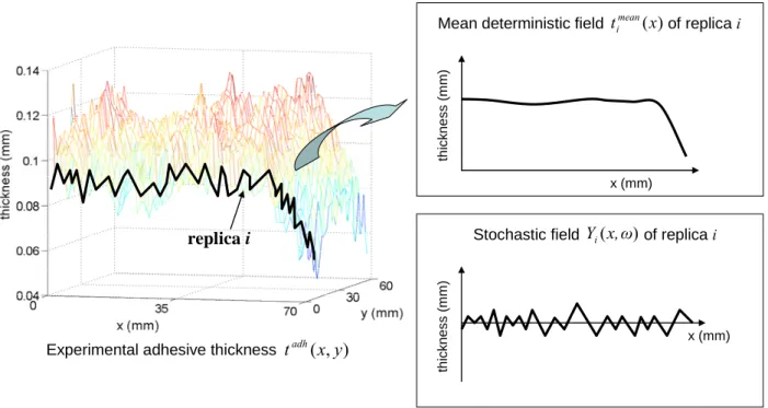
Decomposition of the adhesive thickness is represented in Figure 3. Each replica )

( _i

a i x,ω

t  is smoothed leading to the mean deterministic field tmean(x)

i . Residuals are then obtained by subtracting the mean deterministic field from the full thickness field and are considered as the trajectory Y_i(x,_i),with a mean equal to 0. We can see that the mean deterministic field tmean(x)

i decreases near the free edge of the patch. This is due to the joint fabrication process in this case. This deterministic decrease in the adhesive thickness leads to a stress concentration within the adhesive near the free edge. Uncertain variations may increase this stress concentration. The aim then is to determine the stochastic parameters of the stochastic field Y( ωx, ) from replica trajectories Y_i(x,_i) and to introduce them in a reliability model.

3. Identification of the Y( ωx, ) stochastic field parameters 3.1 Assumptions

Before beginning the identification, some assumptions regarding Y( ωx, ) must be made. Y( ωx, ) is supposed to be a stationary second-order process. As explained above, experimental data are considered as realizations of Y( ωx, ). For each replica i, stochastic parameters have to be identified. The pitch between two abscissae xj , xj+1 is denoted as uj. The

parameters m , _Yi σ_Yi2, )R_Yi(u_k and C_Yi(u_k) can be calculated as:

                  







Using Equations (4), the stochastic parameters can be identified from the experimental measurements (see Section 2). Based on the assumptions described above, the trajectory process is totally defined by the mean mYi, the standard deviation Yi and the autocorrelation

autocorrelation function CYi(u has to be modelled. For this purpose, a negative exponential _k)

function fcor is commonly used:

i u cor k Yi

u

f

u

e

C

(

)



(

)



where u is the distance between two measurement points of the bond and i is a length

parameter.

3.2 Identification of Y ( ωx, ) parameters

The experimental field is developed first following (3) leading to trajectory fields )

( _i

i x,ω

Y  with a mean equal to 0. The decomposition is represented in Figure 3. The identification procedure is applied to trajectory fields Y_i(x,ω_i) in order to identify the mean mY, the standard deviation Y and λ . For the identification of the λ -value, a least i squares-based method is used. As explained above, we consider the stochastic field as 37 replicas. The stochastic parameters of Y ( ωx, ) are calculated as follows:

                







The ratio between the standard deviation and the mean value of the identified parameters characterizes the variability of the results. This ratio, the coefficient of variation (c.o.v.), is chosen to control the result quality. C.o.v. of the standard deviation (respectively of ) is equal to 0.2 (respectively 0.3). Note that we have found similar results in the y-direction. This signifies that the stochastic field Y(x,y,) has isotropic properties. The identification of the mean mY and the standard deviation Y is very well known. However, the identification

stability of the value has to be validated. Especially, we have to check that a c.o.v. equal to 0.3 does not lead to a significant error in the -estimate. In order to check the -identification process stability, a sensitivity analysis is done.

-identification process stability

To validate the -identification process stability, we build first a synthetic sample data set generated from Y ( ωx, ) as it is identified: 64x37 points (leading to 37 replicas of 64 points), a pitch equal to 1.1 mm, L=70 mm. The identified stochastic parameters are also used in the sample data: m_Y 0m and _7.4 106m

Y

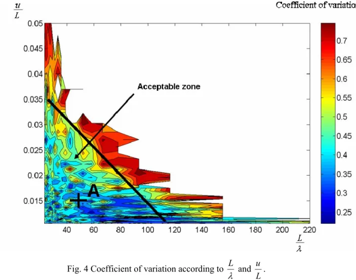
data with 20 different values of uniformly distributed in the range from 0.3 mm to 6 mm. As explained above, for a given -value, c.o.v. of the identified parameter  characterizes the variability in the results and the result quality. The c.o.v. directly depends on 3 parameters: the length L, the pitch u and the -estimate. Therefore, a sensitivity analysis of the c.o.v. is done with respect to the ratio

 L

and the ratio

L u

. The calculated c.o.v. of the -estimate is plotted according to these ratios in Figure 4. An “acceptable” zone is defined in the figure. It corresponds to an error less than 15% in the  value. This constraint corresponds to a c.o.v. less than 0.6. Point A represents the experimental characteristics of our problem (u=1.1 mm, L=70 mm, =1.39 mm). The c.o.v. of the -estimate calculated from Equation (6) is equal to 0.3 which satisfies the criterion.

Now the stochastic parameters of the adhesive thickness field have been identified and validated by the stability of the -identification process. They are now integrated in a reliability model.

4. A combined mechanical and reliability model 4.1 Mechanical model

Some classical models have been developed under some simple assumptions by Volkersen [4] or Hart-Smith [7] for instance. More complex models can be used in order to model non-linear behavior. In this first approach, it has been decided to choose a commonly used model developed by Volkersen [4] in order to highlight the feasibility of the proposed approach. The differential equations which govern the bonded joint behaviour read as follows:          2 2 2 2 ) ( ) ( ) ( ) ( dx x d e x x dx x d p xx p a xz p xx p xx       (7) with:                     xx s p a a s s x p a a E e e G E e E e e G    1 1 (8) ) (x σp

xx , ep and Ex are, respectively, the longiditudinal stress component, the thickness and the Young’s modulus of the bonded composite. σa (x)

xz , ea and Ga are, respectively, the shear stress component, the thickness and the shear modulus of the adhesive. es and Es are,

respectively, the thickness and the Young’s modulus of the substrate. The substrate is subjected to a tensile stress 

xx

σ in the x-direction. This differential equation may be solved

analytically [14] when the thickness is constant. However, as explained above, the adhesive thickness variations are modelled leading to a non-uniform adhesive thickness distribution. We have, therefore, used a finite difference model to solve this differential equation.

4.2 Stochastic model

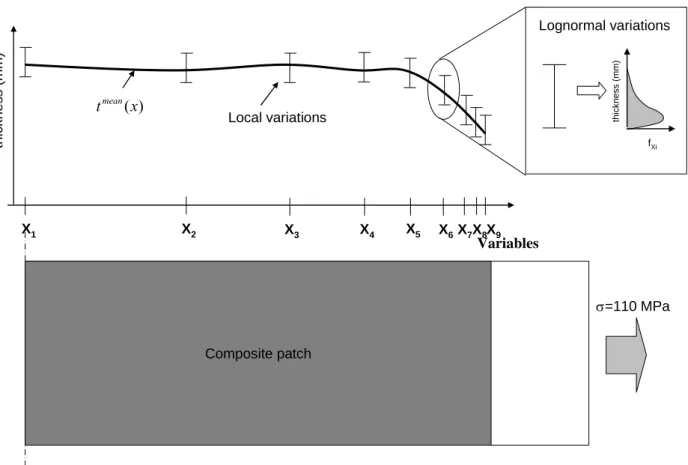
A stochastic model is developed here to take into account the uncertain spatial variations in the adhesive thickness. For this purpose, the adhesive thickness is modelled by a spline curve with nine interpolation points. The abscissae of these points are distributed according to a geometric distribution (see Figure 5). The mean value of the adhesive thickness is determined by the decomposition of the stochastic field (see Section 2.2), and it corresponds to tmean(x)_. These nine thicknesses Xi represent the variables of the problem that constitute the vector X

with the stochastic characteristics identified in section 3. These variables follow a lognormal distribution. The value of shear stress peak in the adhesive a

xz

 (0) enables us to evaluate the bonded joint failure through a limit state which is defined in the next section.

4.3 Reliability model

The stochastic parameters defined in equation (6) are integrated in a reliability model. The limit state G(X)=0 characterizes the bonded joint failure. It is written as follows:

) 0 ( ) ( a xz a S X G   (9)

The shear strength _{S of the adhesive here is equal to 40 MPa. The shear stress in the} a adhesive is calculated with (7). There is failure of the bonded joint when G(X)0. The problem is then to calculate the probability to have G(X)0. The First Order Reliability Method (FORM) here is used [14-15]. It consists in an isoprobabilistic transformation, which transforms the random vector X in the physical space to a random vector U in the standard

Gaussian space where the image of limit state is denoted as H(U)=0. The minimal distance

between the origin and the limit state H(U)=0 represents the reliability index . The closest point on the limit state represents the design point U*. A failure probability Pf is then

approximated from the index :

) Φ( β

P_f   (10)

 represents the standard normal distribution. Determination of the index poses the constrained optimization problem:

0 ) ( subject to , min 2 2 _{ U H U }  (11)

The optimization gives the reliability index  and the failure probability Pf through Equation

(10). For this purpose, the reliability software FERUM v4.0 toolbox is used [18]. Note that the Second Order Reliability Method (SORM) has been used too and results are very close to results calculated with the FORM.

5 Application

5.1 Determination of the failure probability

Simulations are done with the stochastic parameters calculated in Section 3. We consider that the substrate is subjected to a tensile test with a stress equal to 110 MPa. We consider two types of models in order to highlight the influence of uncertain variations in adhesive thickness: the deterministic model and the stochastic model. The deterministic model takes into account the variability of the adhesive thickness without uncertain variations. In this case, the adhesive thickness is equal to tmean(x)_{. The stochastic model takes} into account uncertain variations. In this case, the adhesive thickness is equal to ta( ωx, )_{. Using}

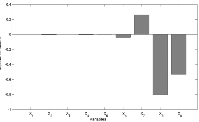
the deterministic model, the shear stress peak can be calculated and is equal to 31.3 MPa, which corresponds to 78% of the strength _{S of the adhesive. Using the stochastic model, the} a failure probability is equal to 83%. We have a significant failure probability although a deterministic calculation equal only to 78% of the adhesive strength _{S . This important result} a clearly shows that the failure probability of the bonded joint is very high (83%) when we consider the uncertain variations in the adhesive thickness despite good results in the deterministic case (78% of the strength _Sa_{). Figure 6 represents the importance factors} defined as follows: ) , , D J D J I x U T x U T    (12) x U

J _, represents the Jacobian of the isoprobabilistic transformation. D represents the diagonal matrix of J_U,xJ_UT_,x . The  –vector is defined as:

) ( ) ( * * U H U H U U    



For the calculation of the importance factors, the reliability software FERUM is used [18]. The importance factors do not have a symmetric distribution. Indeed, they are very important near the right free edge. This is due to the fact that the adhesive works essentially near the free edge of the composite patch. So the adhesive thickness has no influence far away from the free edge. Moreover, the mean adhesive thickness is lower near the right free edge of the joint. So the uncertain variations in the adhesive thickness have more influence on this part of the joint.

5.2 Determination of safety coefficient

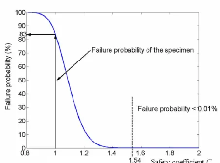
The aim of this section is to determine a safety coefficient in order to have a failure probability lower than 0.01%. Safety coefficient is expressed as a multiplication factor of the adhesive thickness. The idea is to change the initial setting of the adhesive thickness during the joint fabrication process to account for uncertain variations in the adhesive thickness. Calculations are done with safety coefficient Cs integrated in the mechanical model. For this purpose, simulations are done with a safe adhesive thickness eCS(x)

a equal to: ) ( ) (x C e x eC _{s a} aS  (14)

Figure 7 represents the failure probability according to Cs. This figure enables us to analyze the evolution of the failure probability as a function of Cs. value. The failure probability is very high when Cs is lower than 1 and decreases significantly to reach 1.2. Afterwards, this coefficient is determined so as to have a failure probability less than 0.01%. In this case, Cs is equal to 1.54. This signifies that the initial adhesive thickness setting must be multiplied by 1.54 i.e., an adhesive characteristic thickness equal to 0.23 mm instead of 0.15 mm.

6. Conclusion

This work highlights the influence of adhesive thickness variability on the failure of bonded joint. Measurements are done using a three-dimensional measuring machine and experimentally show this variability. An identification procedure enables us to have access to the stochastic parameters of the experimental adhesive thickness field. These parameters are identified and the stability of the identification process is checked. These identified parameters are integrated into a reliability model from which a failure probability of the bonded joint is calculated. Finally, the reliability model is used to determine a safety coefficient to decrease the failure probability to 0.01%. The future of this study lies in improving the mechanical models. In particular, the thickness of the composite adherend can be progressively reduced near the end to reduce the shear stress amplitude. Furthermore, the geometry of the adhesive layer at the free edge (“square end” edges, spew fillets) can be taken into account too. This means that the solution in this more realistic case can probably only be carried out with a numerical model such as a finite element model, despite the problems which are generally encountered when modeling bonded joints with such a tool.. Moreover, surface approximation method may be used in order to increase the accuracy of the failure probability calculation, especially if finite element models are used.

Acknowledgement

The ‘‘Atelier Industriel de l’Aéronautique de Clermont-Ferrand’’ is gratefully acknowledged for its support during this study.

[1] L. Hollaway and M. Leerning, “Strengthening of reinforced concrete structures using

externally-bonded FRP composites in structural and civil engineering”, Woodhead

PublishingLtd, Cambridge, (1999).

[2] A.A. Baker, Composite Structures, 2, 153-164, (1984).

[3] M.J Davis, in: Proceeding of the 3rd. Int. Workshop on Repair of Metallic Structures

using Composites, 4, 1-15, (1995).

[4] O. Volkersen, Luftfahrtforschung, 15, 41–47, (1938).

[5] M. Tsai and J. Morton, Composite Structures, 32, 123–131, (1995). [6] D. Oplinger, Intl. J. Solids Structures, 31, 2565–2587, (1994).

[7] L. Hart-Smith, “Adhesive-bonded single-lap joints”, Tech. Rep. CR-112236, NASA, (1973).

[8] L. Hart-Smith, “Adhesive-bonded double-lap joints”, Tech. Rep. CR-112235, NASA, (1973).

[9] D. Bigwood and A. Crocombe, Intl. J. Adhesion Adhesives, 10, 31–41, (1990) [10] P. Majda and J. Skrodzewicz, Intl. J. Adhesion Adhesives; 29, 396–404, (2009)

[11] G. Ji, Z. Ouyang, G. Li, S. Ibekwe and S.-S. Pang, Intl. J. Solids Structures, 47, 2445– 2458, (2010)

[12] R. Kahraman, M. Sunar and B. Yilbas, Mater. Process. Technol., 205, 183–189, (2008) [13] A. A. Taib, R. Boukhili, S. Achiou, S. Gordon and H. Boukehili, Intl. J. Adhesion Adhesives, 26, 226–236, (2006)

[14] M. Lemaire, “Structural Reliability”, John Wiley & Sons, (2009)

[15] O. Ditlevsen, and H.O. Madsen, “Structural Reliability Methods”, John Wiley and Sons, (1996)

[16] C.G. Bucher and U. Bourgund, Structural Safety, 7, 57-66, (1990).

[18] J.-M. Bourinet, C. Mattrand and V. Dubourg, in: Proceedings of the 10th International

Table 1 - Mechanical properties of the materials1. Ex (GPa) Ey (GPa) (-) xy Gxy (GPa) S (shear strength) (MPa) Composite 141 10 0.28 7 80 Aluminium 70 - 0.32 - - Adhesive 4.2 - 0.3 - 40 1 _E

x (respectively Ey) corresponds to the Young’s modulus in the x-direction (respectively in the y-direction). xy

Fig. 2 Scheme of the decomposition of the experimental thickness tadh(x,y).The experimental thickness tadh(x,y) presents two types of variations: the first is global and is represented by the mean deterministic field tmean(x)

i for each measure in the x-direction; the second is modelled by a stochastic field Y_i( ωx, ) for each measure in the x-direction.

replica i x (mm) th ick n e s s ( m m)

Mean deterministic field tmean(x)of replica i

i x (mm) thi c k ness ( m m )

Stochastic field Yi( ωx, )of replica i

) , ( yx tadh

a – Total adhesive thickness tadh(x,y) b – Smoothing example of a replica )

( ωx, ta

i

c – Mean fields tmean(x)

i d – Stochastic fields Yi(x,)

Fig. 3 Results of the adhesive thickness field decomposition tadh(x,y). Each measure ta( ωx, ) i in the x-direction is smoothed in order to obtain the mean fields tmean(x)

i . Then, the stochastic fields Yi(x,) are obtained by subtracting the mean fields timean(x) from the adhesive field

Fig. 4 Coefficient of variation according to  L and L u .

Fig. 5 Stochastic model: variables Xi are considered to model variations in the adhesive

thickness. These variables follow a lognormal distribution and their abscissae are distributed according to a geometric distribution.

Variables X₁ X₂ X3 X4 X5 X6X7X8X9 Composite patch th ickne s s (mm) ) (x tmean Local variations =110 MPa Lognormal variations th ic kn e s s ( m m ) f_Xi

Fig. 6 Importance factors of the Xi- variables. The variables located near the free edge (X7, X8, X9) have significant importance factors. Therefore, their influences on the failure