HAL Id: hal-00951896
https://hal.archives-ouvertes.fr/hal-00951896
Submitted on 27 Feb 2014HAL is a multi-disciplinary open access archive for the deposit and dissemination of sci-entific research documents, whether they are pub-lished or not. The documents may come from teaching and research institutions in France or abroad, or from public or private research centers.
L’archive ouverte pluridisciplinaire HAL, est destinée au dépôt et à la diffusion de documents scientifiques de niveau recherche, publiés ou non, émanant des établissements d’enseignement et de recherche français ou étrangers, des laboratoires publics ou privés.
Sergei Leonov, Stephen Duffull, Andrew Hooker, France Mentré
To cite this version:
Joakim Nyberg, Caroline Bazzoli, Kayode Ogungbenro, Alexander Aliev, Sergei Leonov, et al.. Meth-ods and software tools for design evaluation in population pharmacokinetics-pharmacodynamics. British Journal of Clinical Pharmacology, Wiley, 2015, Special Issue: Population Dynamics, 79 (1), pp.6-17. �10.1111/bcp.12352�. �hal-00951896�
! " # $ % ! & ' # ( )* + !, - - . * ! ' / ! 0 0 11 * % , - . ' 2 * & 3 1! * ! 4 ) ) * 3 " , - . ' * % ' # " / ! + * ' / ! " / ! # .* # 5 " , # " ! ' * ' ! # & .* ) , # 6 * '' * , - . ' ) * / ! 7 + * # " 8, - - . * / ! 0 * . ' / ! + " ) 9* : , - . 9 / " * 3 ; " "/ ) * %! " ! * /!! + * ! ! " )* ! # / / ! + </3= / ! " ! </ = </3/ = ! " ) " " ) " . ! " " ! 7 " ) ) '' " ! + : 8 ) ' 8 + ! " ) ' ! 5 " '' ! " * ! ) 8 " 8 . " '' ' 8 ! ! . ' : ' ! ! 5 ' /3/ ; ! " " . " ' . ' 8 /: * /+ /* / * / > * " / / ! 8 ' ! " ) 8 ! " = ! ! ! 8 ' /3 ! " , = ! ! 5 /3/ ! " ' / ) " ' < ) ' = 8 " ' . " ' % . <7%?= " ' ' 8 8 ! " ! ' " " . ' ! < >= " " ' ! ' 8 " ! > . " . " ! " ! : 8 ' /3 ! " " ) ' /3/ ! " ' 8 ) . ! ' 8 * ' ' 8 * ! 5 ! : ' ! ! 5* ) + " ) ! 5* . " " " " > . 8 ! > . 8 ! ! " 5 ! 8 " < ' ! 5= : ! /3/
! " * ) ' . ' 8 8 . " ! )' * . " ) ! ! ! " 8 ) " ) !
( ' 8 ) ' 8 ! " ' . 8* . " / : @ ! . 8 ' < ) ! . = ' ) A 8 !' ' ) BA 8 !'
Answer to Referees' comments
Referee 1
Comments to the Author
The authors describe how one experimental design can be evaluated by the set of existing optimal design software tools (that all are based on calculation of the FIM). Two design problems based on population PKPD models are studied, and the design evaluations are compared between the tools and with respect to empirical simulations. Data indicate that all tools give similar output. Evaluation of a single design is a fundamental subroutine in search for an optimal design, and the study therefore functions as a software tool quality check.
Major comments
1. What was the motivation for this study? Did you expect the FIM/SE's to vary significantly between the tools? What would be the consequences if they did, for the developer and for the user community? What are the consequences of the presented result, for the developer and for the user community? The authors should clearly address those questions. Since all key developers in the PKPD optimal design area are co-authors I assume that the main audience is the user community and they will definitely require this background information and perspective.
The main motivation of the present work was indeed to confirm that the computation of the FIM and of the expected SE were similar when using the same approximation in different software tool. It was for us a check about the implementation by all software developers. It was not guaranteed that we would get the same results as different programing language were used (Matlab, R), different coding. The case of the PKPD model written in differential equation was also important to check the complex numerical interlink between solving the ODE and making numerical differentiation.
It was indeed done for the user community to convince them that they could use any tool. We have added the following sentence in the introduction:
“The objectives were to show to the user community that very close results would be obtained with any software tool although programmed in different languages and by different authors. This was also studied in the case of a multiple responses ODE model where the numerical imbrication between ODE solver and numerical differentiation is complex. “
2. The description of what differs between the tools with respect to calculation of the FIM is very vague (line 101), and is not clarified in the section "Statistical methods for design in NLMEM". Are there different heuristics involved, or choices of numerical subroutines, or is it an effect of rounding/order of calculation, and where exactly do these sensitive steps occur in the calculation. This must be explained correctly and pedagogically to the audience.
We agree with your comment. Indeed, the calculation of the FIM was not clearly explained in the section “Statistical methods for design in NLMEM". We have thus added details on the calculation of the FIM in this part and more details in an appendix
3. Since all tools seem to perform (about) equally well in the design evaluation, the user community is interested in knowing how the tools perform on optimal design calculations (where design evaluation is a repeatedly called subroutine, and the search typically is a heuristic algorithm - probably with large differences between the tools). That is, for a set of typical
design problems, what range of optimal solutions are reported by the tools, and what are the run times.
We thank the referee and we agree that this would be the next step of this comparison. However before comparing optimization algorithms we wanted to be sure that all the ‘objective functions’, i.e. criterion values were similar.
The following sentence was added/modified in the discussion:
“This first step was necessary before the next work where we will compare results of design optimization. Indeed now that we know that similar criterion across software are obtained we can compare the rather different optimization algorithms that are implemented.”
4. Writing tends to be sloppy and the manuscript should have been more carefully prepared (see the quite substantial list of minor comment below). This makes a non professional impression, and naturally makes me wonder about the quality of calculations, data handling, and table generation. The authors should scrutinize the entire manuscript including all underlying data generation and presentation.
Thank you very much for such a careful review and many constructive comments. We are sorry for the ‘sloppy’ writing partly due from the deadline of the manuscript for the special issue and by so many different authors. In this new version, the final text was revised by two senior native English speaking authors.
5. The existence of a GUI is indicated by yes/no (line 189, table 1). While a "no" is informative a "yes" can mean anything from rudimentary to professional and it would be informative to present a screen shoot of each relevant tool. The concept 'library of model' has the same problem; how complete are the libraries?
We agree with you and we have suppressed the line about GUI in Table 1. With respect to PKPD model we have added the following sentence in the text after quoting the table.
“Globally, for all software tools, the library of PK model includes one, two or three compartment models, with bolus, infusion or first order (oral) administration, after a single dose, multiple doses or at steady state. PK models with first order elimination
and models Michaelis-Menten
elimination are available. Regarding PD models, immediate linear and Emax models and turnover response models are available.“6. The authors refer to Freemat. Does Freemat contain all subroutines necessary for running the Matlab based tools? Has this been tested for all relevant tools?
Freemat does not contain all subroutines for more advanced options like: automatic differentiation, symbolic derivatives, Laplace approximation of Bayesian design criteria and mode based linearization. However, for the comparison in this paper and for “non-advance” FIM calculations/optimizations FreeMat contain all necessary subroutines. We added a sentence specifying some features which is purely Matlab features.
“Some advanced PopED features such as automatic and symbolic differentiation, Laplace approximation of Bayesian criteria and mode base linearization are not available in FreeMat, however all features preented in Table 1 are available in PopED using either FreeMat or Matlab”
7. Line 257-58: Intuitively, more trials are required for the larger model. Here, it is the other way round (N=1000 for the simpler, N=500 for the more complex problem). These choices, presumably implicitly motivated on lines 304-5, must be directly and clearly motivated when presented.
The number of replicates in a CTS should be motivated by the size of the standard errors because they are evaluated as standard deviations of the estimated parameters, more than by the complexity of the model. Those standard errors depend on variability, number of patients and designs.
However we agree that the decision of K =1000 or 500 replicates were not chosen because of that but because of run times. This is now clarify in the article. We have added the following sentence in the respective section :
“Because the CTS was much more time consuming for the HCV PKPD model, we did not perform the estimation with NONMEM and we did only 500 replicates, whereas we simulated 1000 for the warfarin PK model.”
8. The authors compare their data to CTS, and describe how CTS was used for optimal design calculation in the early 90's. It is well known that computing power has dramatically increased since then. Wouldn't CTS be feasible to many optimal design problems today?
Yes, of course the computing power nowadays had increased dramatically since the 1990’s, but nevertheless the developed optimal design software tools are much faster than CTS which make those tools much easier to use for design optimization. For instance for the HCV PKPD model the CTS took 5 days for one design, so that optimization of doses and sampling times would be difficult. The following sentence was added in the discussion of the paper:
“The computing power nowadays had increased dramatically since the 1990’s, but nevertheless the developed software tools are much faster than CTS which make those tools easier to use for design optimization. For instance for the HCV PKPD model the CTS took several days for one design, so that optimization of doses and sampling times would be difficult.”
9. What is the reason for not including NONMEM in example 2?
As answered in comment 7, this was a runtime issue. It took already 5 days with MONOLIX, and we found very similar results with the predicted standard errors, so that the addition of the NONMEM results would have been of low added value.
Minor comments:
Abstract: the abbreviation PKPD is not defined. PKPD is now defined in the abstract.
Abstract: written as -> defined as. This has been replaced.
Abstract: standard errors (SE) -> standard errors (SE) of the parameters. This has been modified.
Abstract: For most PKPD model -> For most PKPD models. This has been modified.
Line 47-49: Given that the audience is the user community, many readers will probably stop reading after this rather technical sentence in the early Introduction. We agree with your comment and we have simplified the sentence.
Line 50: using -> by. This has been modified.
Line 51: 'seen'. Is it empirically demonstrated for several instances or proved? It is an important result in the Theory of Optimal Experiment. We have thus modified the sentence and added a new reference, the book entitled “Optimal Design for Nonlinear Response Models” written by Fedorov & Leonov.
Line 63. Be consequent: 1970's vs 90's on Line 66. See also rest of the manuscript. This has been modified in the entire document.
Line 70. 'several' means more than 2. We have added now more references.
Line 71: peak and through design is not explained. This was indeed an error. It is “trough” and not ‘through’. We have replaced the word.
Line 72: In 1999 -> From 1999 (?).This has been modified.
Line 85: What does 'The FIM was presented for a' means? This has been clarified.
Line 85: A FIM cannot derive optimal designs; an algorithm may. This has been clarified.
Line 87: 90's'. This has been modified.
Line 97: 'and have presently...', strange grammar. This sentence has been removed.
Line 108: model -> models. This has been corrected.
Line 116: you write that a design 'consists' of N subjects... I thought a study design specifies the number of subjects (as well as other things). The sentence has been rewritten.
Line 119: It’s very confusing when you write about elementary designs that can be divided into vectors of elementary designs (I’m happy you exit this recursion after two steps). This must be explained more pedagogically.
We think it is valid to have a full definition of the multi-response NLMEM model in this paper, however we have rewritten this part to be more comprehensible.
Line 120: when using 'e.g.', 'etc.' is redundant. This has been corrected.
Line 126: l is undefined. l is now defined.
Line 131: i should be in italics This has been modified.
Line 150: lambda is not properly defined. Lambda is now defined clearly.
Line 157: matrix A, and B -> matrices A and B. This has been modified.
Line 168: no institution for PkStaMP is given. In reference to comments from the reviewer 3, we have removed all institutions.
Line 176: Allocation- Matlab -> Allocation – Matlab. This has been modified.
Line 181-82: GUI has already been defined. This has been corrected.
Line 187. remove ',..'. This has been removed.
Line 189: GUI has already been defined. This has been updated.
Line 198: 'expression', don't you mean 'calculation'?. This has been updated.
Line 200: remove 'option'. This has been removed.
Line 200: 'latest' -> 'latter'. This has been updated.
Line 209: The Wald test has not been introduced earlier and deserves a reference. Reference has been added.
Line 216: SE -> SEs. This has been updated.
Line 219: Either use warfarin or Warfarin, don't mix. Check the entire manuscript. This has been updated to use “warfarin”.
Line 219: based on -> based on a. This has been updated.
Line 229: even though HCV was introduced in the abstract it is useful to write it out the first time here as well. This has been updated.
Line 230: Same -> The same. This has been updated.
Line 232: remove '('. This has been removed.
Line 234: Introduce the abbreviation ODE on line 106. This has been updated.
Line 235: why C(t) but all other variables without (t)? This has been updated.
Line 242: (b,p,c,d,n) doesn't agree with information in Table 3. This has been replaced bv (p,d,b,s) and eta (fixed parameter) has been removed (in Table 3 also) to improve clarity.
Line 253: SAEM is undefined. This has been added.
Line 260: why is virtually over lined? This has been removed.
Line 342: lot's -> lots. This has been modified.
Figure legend 1: simulation -> simulated. This has been modified.
Figure legend 2: simulation -> simulated. This has been modified.
Table 1 footnote: remove space in front of colon. This has been modified.
Table 1 footnote: The use of capital first letter seems random. Be consistent and check the entire manuscript. This has been updated for the entire manuscript.
Table 2: Parameters -> parameters. This has been updated.
Updated
Table 2: Is ka the same as Ka?. This has been updated to “ka”.
Table 2: Consequently use a fixed number of value figures (not 1 OR 2). This has been updated.
Table 3: Parameters -> parameters. This has been updated.
Table 3: Consequently use a fixed number of value figures (not 1 OR 2). This has been updated.
Table 3: don't use both the units mL and L in the same list of model parameters. This has been updated.
Table 3: don't use both ^-1 and / to indicate denominators. We agree with your comment but to be more clarify and because “¨-1” is used only once for the fixed constant c, we have kept this notation.
Table 3: remove the space before 'ug/L' for the parameter Beta_EC50. This has been modified.
Table 4: Consequently use a fixed number of value figures (not 2 OR 3). We believe its already one decimal throughout the table.
Table 4: RSE -> RSEs. This has been updated.
Table 5: Consequently use a fixed number of value figures (not 1 OR 2 OR 3). This has been updated.
Table 5: predicted SE for HCV model -> predicted SEs for the HCV model parameters. This has been updated.
Referee 2
Comments to the Author
This is an interesting paper which provides valuable discussion on approaches and tools for design of clinical pharmacology studies. As such it is topical and of interest to BJCP readership. However, the introduction which gives the background to the problems discussed needs to be re-focused and also there is some notation throughout the manuscript which is not defined. In addition, statements on “What is already known about the subject?” and “What this study adds?” are missing.
Specific comments:
p.3, line 45: Please add reference. We have added three initial and important references on design for nonlinear models
p. 3, lines 49-51: The sentence needs to be re-phrased. This has been updated.
p.3, lines 55-58: Needs re-phrasing. This has been updated.
p. 3, lines 58-60. Expand on what advantages Bayesian design offers. It is done very succinctly and not clear to general/non-specialised audience. This has been expanded by adding an example and references to papers using Bayesian designs.
“Some work was also done for Bayesian design, when a priori values of the distribution of the parameters are given, and individual parameters are estimated using the maximum a posteriori probability (MAP). This will optimise individual designs given e.g. a population prior and is suitable for e.g. therapeutic drug monitoring designs (8, 9)”
p. 3, line 70-72. Again please expand on these points as it will show the value of using CTS and/or OD prior to study conduct. This will help to provide the background to the tools comparison. We agree with your comment and we have thus added a line in the paragraph with an example of a drawback with CTS.
p.4, line 105: “straightforward”, please describe it, i.e. one compartment first order absorption and elimination PK model.... This paragraph has been rewritten and completed by an accurate description of the models for both examples.
p.6-7: My main issues is that the descriptions of the model part (up and including to Eq.6) is not the general case from which then the specifics (with assumptions, etc) will be derived. Further in the manuscript multiple responses (balanced, unbalanced) with correlated responses, error terms and full or diagonal omegas will be discussed. Yet, here where a specific case, i.e. diagonal matrix, is specified. The authors need to present and start with the most general model and FIM description and in the user cases (and discussion on tools comparison) refer to how the general case was simplified.
We agree with your comment that a complete general case will be most accurate and possibly preferable, but we believe that a full general notation of the FIM might be overly complicated in this software comparison paper. However we have updated references and added comments were we make assumptions and we believe this will guide the more technical reader to the source of information. According to correlated responses they are implicitly correlated in the FIM if they share common parameters, if e.g. PK is driving PD. We also believe that we have specified a general framework for unbalanced/balanced designs, see equation (1-3) e.g. where individuals can have different number of sampling points between responses.
p.6, Eq. 4: Make use of fk, which is already defined, in the bracket expression for hk . The hk does not
necessarily depend on fk.
p.6, line 141: u not defined. It is defined right here but indeed it seems to be confusing. We thus modified the sentence by defining correctly u as the dimension of the vector of the fixed effects.
p.6, line 142: v not defined. As for the previous comment, we have added some explanations about v.
p.6, line 144: Only diagonal matrix defined, yet in the discussion and comparison section, full and
diagonal are discussed. Similarly, no correlation between responses defined, yet in tables, figures and text it is discussed. You could refer to the previous comment on page 6-7.
p.8, line191: “unbalanced” not introduced in methods section, please add. Indeed, we have thus introduced this term in methods section during the description of a population design of multi-response.
p.9, line 227: Please revised this sentence. The paragraph has been rephrased.
p. 9, line 229: Define HCV abbreviation. This has been modified.
p. 9, line 229: What is the administration frequency? Once a week, very week for how long? Or other?
We thanks for your comment. Indeed the dosing schedule was not clearly defined. We have edited the text. It is a one-day infusion, repeated once a week for four weeks
p. 9, lines 230-231: Here mention that it is balanced design and also the sentence is not finished, is something missing? This has been modified (see the response to the previous comment).
p. 10, line 242: “other seven parameters”, please name them here to ease the reader. Are they δ, s, d, ka, ke, I and EC50? We have named the other seven parameters per your suggestion; they are now ka, ke, Vd;
EC50, n,
δ
, c.p. 11, lines 272-273. Give some explanation (maybe in the discussion section) as to why this is important.
We have added the following paragraph in the discussion
“It seems that when using a FO approximation for computation of the FIM, linearization around some values for the fixed effects, which are then no longer considered as parameters, is the best approach which leads to the block matrix”
p. 12, lines 298-302: All the stated possible reasons for the differences, i.e. differential eq solvers,
numerical derivate methods, step, tolerance, type of ODE solver can be controlled for in the evaluation as all software use MATLAB, except PFIM. Please explain.
This is true but we did not want to constraint all the developers of MATLAB software to implement exactly the same computation, in that case our comparison of software would have been meaningless. It could e.g. be differences that some software uses the backslash operator to calculate matrix inverses, others the inv() function. Some might per default use complex derivatives or even automatic differentiation which is implemented on top of the Matlab interface. Some might have analytic solutions for the derivative of the standard error models (homoscedastic, heteroscedastic) and others numerical differentiation. Therefore, even though Matlab is used in the majority of software, it is hard to fine tune each software so that numerical results are accurate between software up until the Xth decimal. Still the results are very similar which is, as stated in the discussion, an indication of robust approaches in all software.
“These small differences could be seen even across the MATLAB computations of the FIM. Indeed we did not impose to use exactly the same implementation of the various steps across software, hence the need of the present comparison”.
p. 13, line328: Remove “that”. This has been removed.
Referee 3
Comments to the Author
The authors have presented an interesting and informative comparison of currently available optimal design software packages. The manuscript is well structured and the take-home message is clear. I have provided the following comments for clarification/improvement of a few outstanding issues:
Major comments:
1) There are sections of the manuscript where the English is rather fragmented (e.g. the conclusion). Please proofread the manuscript with a focus on grammar.
Thank you very much for such careful review and many constructive comments. We are sorry for the ‘sloppy’ writing partly due from the deadline of the manuscript for the special issue and by so many different authors. In this new version, the final text was revised by two senior native English speaking authors.
2) As the focus of this paper is on the application and comparison of various optimal design software packages, and not on theoretical developments, the authors should consider replacing the "Statistical Methods for Design in NLMEM" section with a general description of D-optimality in the context of nonlinear mixed-effects models, and place the full technical details in a supplementary file or appendix. This modification would require further revision of subsequent sections to ensure notation is consistent within the main text. I understand that this may require a reasonable amount of work, but I believe this alteration would make the manuscript more palatable for the BJCP audience.
We have decided to keep this section in the main manuscript, as we think that we did not make very complex statistical development and as this remark was not made by the associate editor or other reviewers who wishes more development.
We have also added an appendix with more details on the FIM for FO approximation and we have added references for more complex approximations of the FIM as asked by other referees.
3) Please justify the choice of the designs used for evaluation.
The designs were those used in the publications of the chosen example. This was added in the text.
4) The second paragraph of the "Software Description" section should be moved to the "Comparison of software for design evaluation" section, or removed.
The second paragraph of the software description has been moved to the beginning of the section “Comparison of …”. We have thus modified the presentation of the outline of the paper in the introduction.
5) Why was the CTS for the PK example perfomed in both NONMEM and Monolix, whereas the CTS for the PKPD example only performed in Monolix? For the latter, I assume this choice was made due to computational economy. Please justify this decision.
“Because the CTS was much more time consuming for the HCV PKPD model, we did not perform the estimation with NONMEM and we did only 500 replicates, whereas we simulated 1000 for the warfarin PK model.”
6) Please state the variance-covariance structure (full or block diagonal) used in the CTS. Also, please make a comment in regards to theory (e.g. in line/out of line) when comparing the expected full FIM criterion to the observed empirical criterion.
For the CTS a diagonal variance-covariance matrix of the random effects was used. Then to compute the empirical variance-covariance matrix, the full variance-covariance matrix of all the estimates was computed, not as two separate blocks for fixed effects and random components. So that results from observed criterion were obtained with a full matrix.
This has been added in the text in the section “Comparison of software….” at the end of the part “methods”.
7) I assume the choice of 500 runs for the CTS of the PKPD example was made due to computational expense. Please clarify. Also, if at all possible, an extra 500 runs would provide consistency with the 1000 runs for the PK example.
See answer to comment 5).
8) Table 5 should report \%RSEs, like in Table 4.
This was corrected.
Minor comments:
1) Line 57: "... not favoured by pharmacologist who wanted to study the PK of the drug" could be replaced by: "not favoured by pharmacologists interested in exploring complex PK models". This has been changed.
2)
Line 71: Please clarify "peak and through design". This was indeed an error. It is “trough” and not ‘through’. We have replaced the word.3) Please delete the first sentence of the "Software Description" section. The sentence has been deleted.
4) In the "Software Description" section, please unbold the names of the software packages. In the brackets following the acronyms, please replace the bold letters with underlined letters. Also, it is not necessary to list the affiliations with each package.
We have “unbolded” the names of the software and affiliations have been removed, as suggested by another reviewer.
5) When defining the PKPD example, it would be helpful to provide a description of what the I, T and W compartments represent, as well as some brief descriptions of the PD parameters (s, b, d, etc.). This information could be presented in a supplementary file or appendix (see major comment 2).
We agree with your comment and we have completed the description of the PKPD model and added references in the manuscript.
6) I definitely agree with the suggestion to run a CTS of the final optimal design. The authors could also mention that CTS can assess bias, as D-optimal design focuses on parameter precision. I do not entirely agree with the statement "this (CTS at a specified design) should not be computationally onerous". This is indeed true for simple models, however, for more complex models (like the PKPD example), this can take some time, especially if you have to run the CTS locally. Please consider revising this statement.
In the discussion, the paragraph has been completed as follows: “…computationally onerous compared to “optimise” designs with CTS. Moreover, using a CTS study of the final design makes it possible to assess the bias which is not evaluated by the FIM, assuming an unbiased maximum likelihood estimator.”
7) Table 1 - please add symbols (superscripts) to the acronyms in the table and incorporate these symbols into the footnotes. Also provide footnotes for Omega and Sigma, and use "covariance" rather than "cov".
This has been corrected.
8) Tables 2 and 3 - please add footnotes to define betas, omegas and sigma, as well as CL/F, V/F, etc. Alternatively, add a footnote that states something like "as defined in section X" (i.e. where the parameters are defined in the text, supplementary file or appendix).
This has been added.
9) Table 4 - see comment above regarding footnotes. Also, revise the title of the table to "Fisher Information Matrix (FIM) predicted ..." and replace "Block diagonal" and "Full" with "Block diagonal FIM" and "Full FIM", respectively.
This has been updated.
10) Table 5 - again see comments above regarding footnotes.
This has been updated.
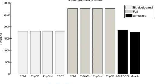
11) Figures 1 and 2 - please provide a footnote stating that the criterion from the simulations was the average/median criterion from the 500 or 1000 simulations. Also, for Figure 1, please provide a more informative label than "NM FOCEI" for the NONMEM simulations, or provide a footnote defining the abbreviation.
The simulation criterion is calculated using the empirical covariance matrix from all the estimates in the CTS, not the median/average of the observed FIM for each dataset (each simulation). We added a criterion definition in the methods section. Footnote for NM FOCEI added.
1 3
Authors
4
Joakim Nyberg (1), Caroline Bazzoli (2), Kay Ogungbenro (3), Alexander Aliev (4), Sergei Leonov (5), 5
Stephen Duffull (6), Andrew C. Hooker (1), France Mentré (7) 6
(1) Department of Pharmaceutical Biosciences, Uppsala University, Uppsala, Sweden; 7
(2) Laboratoire Jean Kuntzmann, Département Statistique, University of Grenoble, France ; 8
(3) Centre for Applied Pharmacokinetic Research, School of Pharmacy and Pharmaceutical Sciences, 9
University of Manchester, Manchester, United Kingdom; 10
(4) Institute for Systems Analysis, Russian Academy of Sciences, Moscow, Russia; 11
(5) AstraZeneca, Wilmington, DE, USA; 12
(6) School of Pharmacy, University of Otago, Dunedin, New Zealand; 13
(7) INSERM U738 and University Paris Diderot, Paris, France; 14
15
Submitting Author and Corresponding Author 16
France Mentré, [email protected] 17
18
Running head: Softwares for design evaluation in population PKPD 19
Keywords: optimal design, population design, Fisher information matrix, nonlinear mixed effect
20
models, population PKPD, PFIM, PkSaMp, PopDes, POpED, POPT. 21
Word count: 3800
22
Numbers of tables and figures: 5 tables and 2 figures
2 development and in academic research. Hence designing efficient studies is an important task. 26
Following the first theoretical work on optimal design for nonlinear mixed effect models, this 27
research theme has grown rapidly. There are now several different software tools that implement an 28
evaluation of the Fisher information matrix for population PKPD. We compared and evaluated five 29
software tools: PFIM, PkStaMP, PopDes, PopED, and POPT. The comparisons were performed using 30
two models: i) a simple one compartment warfarin PK model; ii) a more complex PKPD model for 31
Pegylated-interferon (peg-interferon) with both concentration and response of viral load of hepatitis 32
C virus (HCV) data. The results of the software were compared in terms of the standard error values 33
of the parameters (SE) predicted from the software and the empirical SE values obtained via 34
replicated clinical trial simulation and estimation. For the warfarin PK model and the peg-interferon 35
PKPD model all software gave similar results. Of interest it was seen, for all software, that the simpler 36
approximation to the Fisher information matrix, using the block diagonal matrix, provided predicted 37
SE values that were closer to the empirical SE values than when the more complicated approximation 38
was used (the full matrix). For most PKPD models, using any of the available software tools will 39
provide meaningful results, avoiding cumbersome simulation and allowing design optimisation. 40
3 techniques started in the 1960’s, followed by estimation of dose-response and of pharmacodynamics 44
(PD) models. At around the same time mathematical approaches to defining the problem of optimal 45
design for parameter estimation in nonlinear regression was addressed (1-3). However this did not 46
reach the PK literature until some 20 years later (4). The problem was not only to draw inference 47
from data but also to define the best design(s) for estimation of parameters using maximum 48
likelihood or other estimation methods. For this purpose, the Fisher Information matrix (FIM) was 49
used to describe the informativeness of a design, i.e. how much information the design has in 50
relation to parameter estimation. Typically in PK the FIM is summarized by its determinant and 51
maximising the determinant, termed D-optimality, is equivalent to minimising the asymptotic 52
confidence region of the parameters, i.e. getting the most precise parameter estimates (5-9). 53
However, beyond theoretical developments, a limitation of individualised optimised designs of PKPD 54
studies is that those designs do not acknowledge population information and hence cannot have 55
fewer sampling times per individual than parameters to estimate. In addition, optimal designs with a 56
large number of observations per patient will have replicated optimal sampling times; which were 57
not favoured by pharmacologists interested in exploring complex PK models. Some later work also 58
explored Bayesian designs, where a priori distributions of the parameters were considered, and 59
individual parameters were estimated using maximum a posteriori probability (MAP). Optimal 60
designs for MAP estimation optimise individual designs given prior population information and are 61
suitable for e.g. therapeutic drug monitoring designs (10, 11). Since 1985, the software Adapt 62
(https://bmsr.usc.edu/software/adapt/) has included methods for optimal design in nonlinear 63
regression using several criteria for MAP estimation. 64
The population approach was introduced by Sheiner et al. (12) for PK analyses in the late 1970’s and 65
since the 1980’s there has been a large increase in the use of this approach as well as extensions to 66
PKPD. Estimation was mainly based on maximum likelihood using nonlinear mixed effects models 67
(NLMEM) thanks to the software NONMEM. To our knowledge the first article studying the impact of 68
a ‘population design’ on properties of estimates was performed in early 1990’s by Al Banna et al. (13) 69
for a population PK and a population PKPD example. In this work the author used clinical trial 70
simulation (CTS) to explore possible designs. The authors studied the influence of the balance of 71
number of patients, number of sampling times and locations of the sampling times on the precision 72
of the parameter estimates. Several papers, all using CTS, were published (14-16) showing that some 73
designs could be rather poor (for instance peak-and-trough sampling design), and that very sparse 74
4 information, should be performed to “anticipate certain fatal study designs, and to recognize 77
informative ones”. 78
Using CTS for design evaluation requires a large number of data sets to be simulated and then fitted 79
under each proposed design which is computationally expensive. However, since CTS is a user driven, 80
heuristic approach, then it can miss important regions of the design space because only a fixed 81
number of designs are investigated. Subsequently it was suggested to use the FIM in NLMEM to 82
predict asymptotic standard errors (SE) and define optimal designs without the need for intensive 83
simulations. Because the population likelihood has no closed-form expression the proposed 84
approach for defining the population FIM was to use a first-order linearisation of the model around 85
the random effects (which is the same as used for the first-order (FO) estimation methods). This 86
approximation results in a mixed effect model where the random effects enter the model linearly 87
(rather than nonlinearly) and hence has properties that are similar to linear mixed effects model. The 88
expression for the population FIM was first published in Biometrika in 1997 (18). In this work the FIM 89
was derived for a population PK example and an algorithm was proposed to optimise designs based 90
on the population FIM. This paper launched the new field of optimal design for nonlinear mixed 91
effects models. It has been quoted in the section ‘other influential papers of the 1990’s’ in a review 92
in Biometrika (19). 93
Since 1997 several methodological papers from various academic teams have published different 94
extensions, for instance robust designs, sampling windows, compound designs, multiple response 95
models, methods for discrete longitudinal data, and other approximations of the FIM, etc. Most 96
importantly, the derivation of the expression of the FIM was implemented in several software tools, 97
the first one PFIM (20) in 2001 appeared simultaneously in both R (http://www.r-project.org/) and 98
Matlab (http://www.mathworks.fr/products/matlab/). This was followed by POPT (21), and later to 99
incorporate an interface version WinPOPT, PopED (22), PopDes (23) and PkStaMp (24). There are 100
now five different software tools, all implementing the first-order approximation, with some tools 101
implementing one or several other approximations. These tools for designing population PKPD 102
studies are gaining popularity. In a recent study performed among European Federation of 103
Pharmaceutical Industries and Associations members’ (25), it was found that 9 out of 10 104
pharmaceutical companies are using one of these software tools for design evaluation or 105
optimisation, mainly in phases I and II. 106
5 in terms of FIM and predicted SE values. The same basic approximations were used in each software, 109
and the comparison was performed for two examples: (1) a simple PK example described by a one-110
compartment model with first-order absorption and linear elimination and (2) a more complex PKPD 111
example where the PD component is defined by a system of nonlinear ordinary differential equations 112
(ODE). The objective was to explore the results from different software tools and to compare results 113
against those obtained using CTS. We wanted to show the user community that similar results would 114
be obtained with any software tool although programmed in different languages and by different 115
authors. This was also studied in the case of a multiple responses ODE model where the numerical 116
imbrication between ODE solver and numerical differentiation is complex. The results were provided 117
by the software developers, all authors of this article, who were given the equations of the models, 118
the values of the parameters and the designs to be evaluated. Results were compared to those 119
obtained by CTS. 120
The article is organized as follows: first the description of the population FIM for NLMEM, second a 121
description of the various software tools, and then an evaluation of the two examples. As no design 122
optimisation was performed in the present study, no optimisation characteristics or algorithms are 123
described. 124
125
Statistical methods for design in NLMEM
126
A design for a multi-response NLMEM is composed of subjects each with an associated 127
elementary design
ξ
( = ). Hence a design for a population of subjects can be described 128 as 129(
ξ
ξ
)
Ξ = (1) 130Each elementary design
ξ
can be further divided into sub-designs 131(
)
ξ
=ξ
ξ
(2)132
with
ξ
, = being the design associated with the kth response. (e.g. drug concentration,133
metabolite concentration, effect). It may thus be possible to have all responses measured at different 134
times, termed an unbalanced design. 135
6 at which the response variable is measured.
138
An elementary design
ξ
can be the same within a group of subjects ( = ). Using a 139similar notation for the complete population design
Ξ
in a limited number of groups of different 140elementary designs gives: 141
[
] [
]
(
ξ
ξ
)
Ξ = (3)
142
where the total number of subjects in the design, , is equal to the sum of the subjects in the 143
elementary designs. At the extreme, each subject may have a different design, , or each subject 144
may have the same design, = 1. 145
In a NLMEM framework with multiple response, the vector of observations for the ith subject is 146
defined as the vector of K different responses: 147
= (4)
148
where , = is the vector of nik observations for subject i and response k modelled as
149
(
θ ξ
)
(
θ ξ ε
)
= + (5)
150
where fk(.) is the structural model for the kth response,
θ
is the ith subject’s parameter vector, hk(.) is151
the residual error model for response k, often additive (h=
ε
), proportional (h=( )
⋅ε
) or a 152combination of both,
ε
is the residual error vector for response k in subject i. In this paper additive 153(homoscedastic) or proportional (heteroscedastic) error models will be used in the examples so that 154
only one residual variance parameter is defined for each response. To simplify notation we assume 155
that
ε
are normally distributed and independent between responses (which is not necessary, see 156e.g. (26, 27)) with mean zero and variance Σk=diag(
σ
). The individual parameter vectorθ
, with157
parameter(s) that might be shared between responses, is described as 158
(
)
θ
=β
(6)7 parameter. We assume that bi is normally distributed with a mean of zero and a covariance matrix
162
of size . Again, to simplify notation we assume a diagonal (which is not necessary, see e.g. 163
(18, 27-29)) interindividual covariance matrix ( ) with diagonal elements (
ω
ω
). The vector of 164population parameters is thus defined as 165
[
]
ψ
=β λ
= β ω
ω σ
σ
(7)166
where
λ
= ω
ω σ
σ
is the vector of all variance components. 167The population Fisher information matrix
(
ψ
Ξ)
for multiple response models with the 168population design
Ξ
Ξ
Ξ
Ξ
is given by: 169(
ψ
)
(
ψ
)
ψ ψ
∂ Ξ = − ∂ ∂ (8) 170where
(
ψ
)
is the log-likelihood of all the observations Y given the population parametersψ
. 171Assuming independence across subjects, the log-likelihood can be defined as the sum of the 172
individual contribution to the log-likelihood:
(
ψ
)
(
ψ
)
=
=
∑
. Therefore, the population 173Fisher information matrix (calculated using the second derivative of the log-likelihood) for N subjects 174
can also be defined as the sum of the N elementary information matrices
(
ψ ξ
)
computed for 175 each subject i: 176(
ψ
)
(
ψ ξ
)
= Ξ =∑
(9) 177In the case of a limited number of groups (where each individual in a group share the same design), 178
as in Equation (3), the population FIM is expressed by: 179
8 181
For one subject, given the design variables
ξ
and the NLMEM model, the FIM is a block matrix 182defined as: 183
(11) 184
where
(
β ξ
)
=
is the block of the Fisher matrix for the fixed effectsβ
and 185(
λ ξ
)
=
is the block of the Fisher matrix for the variance componentsλ
. 186When a standard FO approximation of the model is performed (see appendix), then the distribution 187
of the observations in patient i with design ξi is approximated by
(
)
. Expressions for the188
population mean and population variance are given in the appendix. Then the following 189
expression for blocks , and are obtained (18, 30, 31), ignoring indices i for simplicity : 190
β
β
β
β
− − − ∂ ∂ ∂ ∂ ≅ + ∂ ∂ ∂ ∂ with =( )
β
191λ
λ
− −∂
∂
≅
∂
∂
with =( )
λ
(12) 192λ
β
− −
∂
∂
≅
∂
∂
with =( )
λ
=( )
β
193 194This expression of the FIM (eq. 12) will be referred to as the full FIM in this paper. 195
If the approximated variance is assumed independent of the typical population parameters
β
, the 196matrix will be zero and the matrices and will instead be defined as: 197
β
β
− ∂ ∂ ≅ ∂ ∂ with =( )
β
(13) 1989 200
which will be termed the block diagonal FIM in the following. The explicit formula for
(
β ξ
)
201using the block diagonal form is given in the appendix. More information about the derivation of the 202
FIM or other approximations are reported in (27, 28, 30, 32-34). 203
204
Software description
205
There are presently five software tools that implement experimental design evaluation and 206
optimisation of the FIM for multiple response population models. The five software tools are (in 207
alphabetical order) : PFIM (35), PkStaMp (24), PopDes (23), PopED (27, 31) and POPT (21). Four of 208
them have been developed by academic teams. 209
PFIM (Population Fisher Information Matrix) is the only tool that is using the software R, the other 210
software packages have been developed under the numerical computing environment MATLAB. The 211
first version of PFIM appeared in 2001 and since this date several releases have been issued. It is 212
available at www.pfim.biostat.fr. A graphical user interface (GUI) package using the R software 213
(PFIM Interface) is also available but does not include recent methodological developments. 214
Pk StaMP (Pharmacokinetic Sampling Times Allocation – Matlab Platform) is a library compiled as a 215
single executable file which does not require a MATLAB license. The developers can share the stand-216
alone version with anyone interested. PopDes (Population Design) has been developed at the 217
University of Manchester and this application software is available atwww.capkr.man.ac.uk/home 218
since 2007. PopED (Population optimal Experimental Design), freely available at poped.sf.net, 219
consists of two parts, a script version, responsible for all optimal design calculations, and a GUI. The 220
script version can use either MATLAB or Freemat (http://www.freemat.sf.net)(a free alternative to 221
MATLAB) as an underlying engine. Some advanced PopED features such as automatic and symbolic 222
differentiation, Laplace approximation of Bayesian criteria and mode base linearisation are not 223
available in FreeMat, however all features presented in Table 1 are available in PopED using either 224
FreeMat or Matlab. POPT (Population OPTimal design) was developed from PFIM (MATLAB) in 2001 225
and is constructed as a set of MATLAB scripts. POPT requires MATLAB and can run on FreeMat. This 226
tool can be downloaded on the website www.winpopt.com. All the software tools run on any 227
common operating system platform (e.g. Windows, Linux, Mac). 228
10 Comparison of software for design evaluation
230
As we focus on design evaluation and not design optimisation, we first compared the software tools 231
with respect to a) required programming language, b) availability, c) library of PK and PD models, and 232
ability to deal with: d) multiple response models, e) models defined by differential equations, e) 233
unbalanced multiple response designs, f) correlations between random effects and/or residuals, g) 234
models including inter-occasion variability, h) models including fixed effects for the influence of 235
discrete covariates on the parameters, i) computation of the predicted power. Table 1 is a summary 236
of the comparison of the software with respect to these different aspects. Globally, for all software 237
tools, the library of PK model includes one, two or three compartment models, with bolus, infusion 238
or first-order (e.g. oral) administration, after a single dose, multiple doses or at steady state. PK 239
models with first-order elimination and models Michaelis-Menten elimination are available. 240
Regarding PD models, immediate linear and Emax models and turnover response models are 241
available. 242
Over recent years, those tools have included various improvements in terms of model specification 243
and calculations of the FIM. For all of them, design evaluation can be performed for single or multiple 244
response models either using libraries of standard PK and PD models or using a user-defined model. 245
For the latter, regardless of the software used, the model can be written using an analytical form or 246
using a differential equation system. In the case of multiple response models, population designs can 247
be different across the responses for all the software. Regarding the calculations of the information 248
matrix, the majority of the software can handle either a block diagonal Fisher information matrix 249
(block FIM) or the full matrix (full FIM). Otherwise, only PopDes and PopED allow for calculations for 250
a model with both correlation between random effects (full covariance matrix Ω) and correlation 251
between residuals (full covariance matrix Σ), PKStamp allows full covariance matrix Ω. It is possible in 252
PFIM, PopDes and PopED to use models with inter-occasion variability (IOV) and models including 253
fixed effects for the influence of discrete covariates on the parameters. The computation of the 254
predicted power of the Wald test (30, 36) for a given distribution of a discrete covariate can be 255
evaluated in PFIM, PopDES and PopED frameworks. 256
257 258
Examples
11 FIM and the predicted asymptotic SEs, without design optimisation. This was done to evaluate the 262
core calculations of the FIM. The FIM is evaluated with the full and the block diagonal derivation (eq. 263
12, 13) with the different software tools. 264
In the first example a one compartment PK model (based on a warfarin PK model) with first-order 265
absorption was used (35). The design of that study consisted of 32 subjects with a single dose of 70 266
mg (a dose of 1mg/kg and a weight of 70 kg), and with 8 sampling times post-dose (in hours): 267
[
]
(
ξ
)
(
ξ
)
Ξ =
=
268( ) (
!
)
ξ
=
=
269The residual error model was proportional (h =
⋅
ε
) with a coefficient of variation of 10% ( 270σ
= ) and exponential random effects were assumed for all parameters (=
β
). Table 2 271reports the model parameters and their values. The dose and design are based on (34, 37). 272
For the second example a multiple response PKPD model with repeated dosing was selected with the 273
same design across responses (38). The model describes hepatitis C virus (HCV) kinetics, or more 274
specifically, the effect of peg-interferon dose of 180 μg/week administered as a 24 hour infusion 275
once a week for 4 weeks. The same sequence of 12 sampling times for both PK and PD 276
measurements (in days, post-first-dose) was used for 30 subjects: 277
{
}
(
ξ
ξ
)
(
ξ
ξ
)
Ξ = = 278( ) (
!
"
)
ξ
=
ξ
=
=
279The HCV model is described by the following system of ODEs: 280
12
( )
( )
( )
( )
(
( )
)
( )
( ) ( )
( )
!
!
δ
δ
=
−
=
= −
+
=
=
−
( )
( )
"( )
( )
( )
" "!
!
!
δ
δ
δ
δ
−
=
−
=
−
−
=
+
281 282where
( )
=
( )
is the drug concentration at time t and r(t) is the constant infusion rate. The 283viral dynamics model considers target cells, , productively infected cells, and viral particles, !. 284
Target cells are produced at a rate and die at a rate . Cells become infected with de-novo infection 285
rate e. After infection, these cells are lost with rate δ. In the absence of treatment, virus is produced 286
by infected cells at a rate and cleared at a rate c, for more details see (38, 39). The model for each 287
response in subject i is defined as 288
( )
(
)
(
( )
)
#$
#$
!
ε
ε
=
+
=
+
289An additive error model was assumed for both PK and PD (log viral load) compartments from which 290
observations were drawn with a standard deviation of 0.2. Some of the parameters in the model are 291
fixed ( #$ #$ #$ ). For the other seven parameters ( #$ #$ #$ %&#$"#$
δ
#$ ), log transformation was292
made with additive random effects on the log fixed effect with a variance ω2 of 0.25. All parameters 293
and their values are listed in Table 3. 294
295
Methods
296 297
For each example using each software tool, we computed the FIM based on the FO linearisation, 298
given the parameters and the design. We used both the block-diagonal and the full FIM (not available 299
in POPT). From the FIM, we computed the predicted SE values for each parameter and the 300
13 To investigate the FIM predictive performance, the empirical SE values were also estimated using 303
CTS. More precisely, for each example, multiple data sets were simulated and then fitted using the 304
Stochastic Approximation Expectation Maximisation (SAEM) algorithm in MONOLIX 2.4 305
(www.lixoft.eu) and, for the PK example also with the FOCEI algorithm in NONMEM 7 306
(http://www.iconplc.com/technology/products/nonmem/). Empirical standard errors were derived 307
from the estimated parameters. The empirical D-criterion was computed from the normalized 308
empirical variance-covariance matrix of all estimated parameters,
( )
( ) %
&$'
ψψ
− . Because the 309CTS was much more time consuming for the HCV PKPD model, we did not perform the estimation 310
with NONMEM and we did only 500 replicates, whereas we simulated 1000 replicates for the 311
warfarin PK model. 312
For the CTS, to compute the empirical covariance matrix, the full variance-covariance matrix of all the 313
estimated vectors was computed, not as two separate blocks for fixed effects and random 314 components. 315 316 Results 317 318
For the PK model, the results show no differences between the optimal design software tools when 319
evaluating the FIM using the block diagonal and full form. In the same way, all software reported the 320
same expected D-criterion (Figure 1), and the same expected relative standard errors (RSE) values 321
expressed in % (Table 4). 322
In this example, the block diagonal FIM calculations gave an expected D-criterion that was very 323
similar to the observed D-criterion based on the inverse of the empirical covariance matrix (Figure 1). 324
However, for all software, the block diagonal D-criterion is slightly smaller than the NONMEM FOCEI 325
based criterion. Note that the result from MONOLIX is lower than the expected D-criterions, in line 326
with theoretical expectations the Cramer-Rao inequality (FIM is an asymptotic upper bound on the 327
information). The full FIM predicts considerably more information compared to the simulations 328
(expected D-criterions are larger than the observed values), and predicts total information that is 329
farther from the empirical values than the block diagonal calculations. The same trends are evident 330
when looking at the RSE values, reported in Table 4. Good agreement between the CTS and the block 331
14 .
333
For the more complicated PKPD model, results are summarized In Figure 2 and Table 5 where RSE (%) 334
are reported. The D-criterion reveals negligible differences between any of the software (Figure 2) 335
and also almost no difference between predicted SE values (Table 5). In this example, as in the PK 336
example, using the block diagonal FIM gave D-criterion predicted values that were very similar to the 337
D-criterion based on the inverse of the empirical covariance matrix (Figure 2). The full FIM predicts 338
considerably more information compared to the simulations (expected D-criterions larger than the 339
observed values) and predicts total information (D-criterion) that is farther from the empirical values 340
than the block diagonal calculations. The same trends are evident when looking at SE values for each 341
parameter (Table 5). We found good agreement between CTS and the block diagonal FIM, while the 342
full FIM predicted higher precision in numerous parameters than observed. 343
344 345
15 The first statistical developments for the evaluation of the FIM for NLMEM to compare and evaluate 347
population designs without simulation were performed in the late 90’s. Since then, five different 348
software tools have been developed. We have compared these tools in terms of design evaluation. 349
Optimisation was not considered in the present work. It should be noted that most software are 350
under active development with regular addition of new features. 351
We compared the expression of the FIM computed by the five different optimal design software 352
packages for two examples. The first example was a simple PK model for which the algebraic 353
solution could be written analytically. When using the same approximation, all optimal design 354
software packages achieved the same D-efficiency criterion and predicted RSE values (%). The second 355
example was more complex, had two responses (both PK and PD measurements) and the model was 356
written as a series of five differential equations. For this example, the D-criterion and RSE 357
comparisons revealed negligible differences between software. The differences could potentially be 358
explained by the use of different differential equation solvers, methods of implementing multiple 359
response calculations, methods for computing numerical derivatives, tolerance levels for ODEs and 360
numerical implementations of e.g. matrix inverses and solving of linear systems, etc. These small 361
differences could be seen even across the MATLAB computations of the FIM. In this work we did not 362
impose the same implementation of the various steps across software, hence the importance of the 363
present comparison. 364
365
In both examples the expected SE values from the block diagonal FIM were close to the empirical SE 366
values obtained from CTS. The runtimes for all software tools were a few seconds compared to 367
minutes (warfarin example) or days (HCV example) for the CTS evaluation. Although computational 368
speed has increased dramatically since the 1990’s, a significant speed advantage is seen with the 369
developed software tools even without considering design optimisation. For instance for the HCV 370
PKPD model the CTS took several days for one design, so that optimization of doses and sampling 371
times would be difficult. 372
In both examples investigated, the block diagonal FIM calculations give an expected D-criterion that 373
is very similar to the observed D-criterion based on the inverse of the empirical covariance matrix 374
and RSE(%) values for parameter match well. In contrast, the full FIM predicts more information 375
compared to the simulations (expected D-criterions larger than the observed values). More 376
discussion on the assumptions beyond the block or full matrix can be found in (33) together with 377
16 no longer considered as estimable parameters and therefore corresponds to the block diagonal 380
matrix, provides the best approach. Also higher order approximations to the FIM are available that 381
may give better prediction of RSE(%) values (27). 382
Results using the simple FO approximation and the block diagonal FIM are very close to those 383
obtained by CTS using both FOCEI and SAEM estimation methods in the two examples. However, 384
since the expected FIM calculation is computing an asymptotically lower bound of the covariance of 385
the parameters, and the calculations are based on approximations, the authors suggest that a CTS 386
study of the proposed final design be performed in order to evaluate the likely performance of the 387
design in the setting in which it is proposed to be used. Since this would be a single CTS at a specified 388
design then this should not be computationally onerous compared to attempting to “optimise” 389
designs using CTS. In addition, using a CTS study of the final design makes it possible to assess the 390
bias which is not evaluated by the FIM. 391
In this first comparison between the software, we did only design evaluation for continuous data and 392
using the simpler FO approximation of the FIM. This first step was necessary before the next work 393
where we will compare results of design optimisation. Indeed now that we know that similar 394
criterion across software are obtained, we can compare the rather different optimisation algorithms 395
implemented. In principle any design variable that is present in the model can be optimised within an 396
optimal design framework. Examples of design variables that can be optimised are measurement 397
sampling times, doses, distribution of subjects between elementary designs, number of 398
measurement samples in an elementary design, etc. How this is done and which design variables can 399
be optimised varies between software, but the independent variable (e.g. measurement sampling 400
times) and the group assignment can be optimised in all software presented in this paper. Results will 401
depend on the assumptions about the model and the parameter values, so that sensitivity studies 402
should be performed to implement ‘robust’ designs, i.e. designs that are robust to the assumed a 403
priori values of the parameters. Approaches for design optimisation using a priori distribution of the 404
parameters were suggested and implemented for standard nonlinear regression and extended to 405
population approaches and should also be compared in further studies. 406
In conclusion, optimal design software tools allow for direct evaluation of population PKPD designs 407
and are now widely used in industry (25). Choice of software can depend on what platform the user 408
has available and what features they are looking since the FIM calculation in the different software 409