HAL Id: hal-02344374
https://hal.archives-ouvertes.fr/hal-02344374
Submitted on 4 Nov 2019
HAL is a multi-disciplinary open access
archive for the deposit and dissemination of
sci-entific research documents, whether they are
pub-lished or not. The documents may come from
teaching and research institutions in France or
abroad, or from public or private research centers.
L’archive ouverte pluridisciplinaire HAL, est
destinée au dépôt et à la diffusion de documents
scientifiques de niveau recherche, publiés ou non,
émanant des établissements d’enseignement et de
recherche français ou étrangers, des laboratoires
publics ou privés.
Ultrafast 3D Ultrasound Localization Microscopy Using
a 32x32 Matrix Array
Baptiste Heiles, Mafalda Correia, Vincent Hingot, Mathieu Pernot, Jean
Provost, Mickael Tanter, Olivier Couture
To cite this version:
Baptiste Heiles, Mafalda Correia, Vincent Hingot, Mathieu Pernot, Jean Provost, et al..
Ultra-fast 3D Ultrasound Localization Microscopy Using a 32x32 Matrix Array. IEEE Transactions on
Medical Imaging, Institute of Electrical and Electronics Engineers, 2019, 38 (9), pp.2005-2015.
�10.1109/TMI.2018.2890358�. �hal-02344374�
Ultrafast 3D Ultrasound Localization
Microscopy using a 32x32 Matrix Array
Baptiste Heiles
1, Mafalda Correia
1, Vincent Hingot
1, Mathieu Pernot
1, Jean Provost
1, Mickael
Tanter
1,*, Olivier Couture
1,*
* These Authors contributed equally to this work
Abstract — Ultrasound Localization Microscopy can map blood vessels with a resolution much smaller than the wavelength by localizing microbubbles. Current implementations of the technique are limited to 2-D planes or small fields of view in 3D. These suffer from minute-long acquisitions, out-of-plane microbubbles and tissue motion. In this study, we exploit the recent development of 4D ultrafast ultrasound imaging to insonify an isotropic volume up to 20000 times per second and perform localization microscopy in the three dimensions. Specifically, a 32x32 elements, 9-MHz matrix-array probe connected to a 1024–channel programmable ultrasound scanner was used to achieve sub-wavelength volumetric imaging of both the structure and vector flow of a complex 3D structure (a main canal branching out into two side canals). To cope with the large volumes and the need to localize the bubbles in the three dimensions, novel algorithms were developed based on deconvolution of the beamformed microbubble signal. For tracking, individual particles were paired following a Munkres assignment method and velocimetry was done following a Lagrangian approach. ULM was able to clearly represent the 3D shape of the structure with a sharp delineation of canal edges (as small as 230 µm) and separate them with a spacing as low as 52µm. The compounded volume rate of 500Hz was sufficient to describe velocities in the [2.5-150] mm/s range and to reduce the maximum acquisition time to 12s. This study demonstrates the feasibility of in vitro 3D ultrafast ultrasound localization microscopy and opens up the way towards in vivo volumetric ULM.
Index Terms— Ultrasound, Microbubbles ULM,
super-resolution, 4D
I. INTRODUCTION
The trade-off between penetration and resolution in ultrasound imaging is a recurring obstruction to deep tissue high resolution imaging. Recently, several studies have demonstrated the possibility to overcome this issue by using contrast enhanced agents to yield separated echoes in the region of interest and localizing them [[1],[2]]. Such
1Institut Langevin, CNRS, INSERM, ESPCI Paris, PSL Research University, 17 rue Moreau, 75012, Paris.
Corresponding Author : Baptiste Heiles, [email protected]
method is comparable to optical localization microscopy, which improved the resolution of optical microscopes by several orders of magnitude [3] . In ultrasound imaging, a similar improvement in resolution obtained through the localization of microbubbles was demonstrated in-vitro by several teams [[4],[5],[6]]. In-vivo, ultrasound localization microscopy has highlighted and separated blood vessels much smaller than the wavelength in the rat brain [[7],[8]], ear [9], kidney [[10],[11]] and in implanted tumor in mice [12]. A comprehensive review of ultrasound localization microscopy and super-resolution was recently published [13]. Although ultrasound localization microscopy was introduced with ultrafast imaging at frame rates beyond 500 Hz [[2],[14]], conventional scanners (<50 Hz) were also used to infer trajectories of microbubbles at lower frame rates.
While disrupting the compromise between penetration and resolution for vascular imaging, ultrasound localization microscopy has introduced new trade-offs. The signal-to-noise ratio of the image is particularly important as it
defines the localization precision of individual
microbubbles, which can attain 2 µm [15]. Such micrometric resolution vastly increases the sensitivity to motion, requiring ultrasound based motion correction algorithms [[8],[10]]. More fundamentally, the localization process requires the passage of microbubbles in each vessels to be observed, leading to a compromise between microbubble concentration, time and resolution [16]. In the end, the quality of the super-resolved image is limited less by the localization precision of the individual microbubbles, but rather by the total number of accumulated microbubble positions or tracks per frame. The localization process collapses if microbubbles are closer than a few wavelengths from each other’s, as their response function interfere together. Consequently, a limited number of scatterers can be separated in each individual image, leading to minutes-long acquisitions to reveal the micron-sized vasculature in each plane. Because of these acquisition times, a plane-by-plane ULM observation of a full organ remains difficult to apply [[7], [12]]. This issue has created major hurdles in the
2
implementation of ULM for organ-wide imaging. Furthermore, other limitations such as out-of-plane motion, projection error of 3D microvasculature in 2D space or non-isotropic information, hampers the retrieval of relevant vascular markers in-vivo. Some of these constraints were lifted with the use of multiple parallel [4]or perpendicular arrays [9], but the observation volume was always restricted to a small volume around a plane or a line, inducing the same problems on a smaller scale.
Geometrically, many more microbubbles can be separated in a volume rather than on a single plane. A succession of 3D acquisitions would therefore permit much shorter imaging times than a plane-by-plane acquisition. Moreover, it would allow motion correction algorithms to be applied in the 3rd dimension. Projection error would be
eliminated and the tracking of microbubbles paths would become isotropic, allowing a micrometric resolution in all directions and instant velocimetry and flow rate measurement. More complex trajectories can be reconstructed as separation of microbubbles in the 3rd
dimension is possible.
Conventional line-by-line ultrasound scanning in 3D is limited in volume-rate to about 10 Hz. Explososcan developed in the 1980s achieves volume rates of 30Hz thanks to parallel receive processing [17], but these volume rates remain low and would make individual microbubbles difficult to track with sufficient temporal resolution in ULM. Thanks to sparse synthetic aperture beamforming, the quest towards real-time 3D progressed over time with a growing number of papers since the 1990s: Lockwood et al [18], Hazard et al [19] proposed using a mechanically scanned linear phased-array, Jensen
et al [20] build a system based on synthetic aperture to
achieve real time ultrasound 3D imaging. Recently, the introduction of 4D or ultrafast volumetric ultrasound imaging has permitted volume acquisition rates in the kHz-range [21]. It opened new possibilities like 3D Doppler imaging [[21],[22]], for making velocimetry measurement in large 3D structures like the heart, human thyroids or the carotid artery. Holbek et al presented an in vivo carotid artery 3D velocity vector study using continuous measurements in one imaging plane [23]. Correia et al. introduced 4-D ultrafast ultrasound flow imaging to access full in vivo volumetric arterial blood flow distribution in a single heartbeat at the common carotid and bifurcation carotid arteries levels [24]. Gennisson et al introduced 4D ultrafast imaging for 3D Shear Wave Elastography [25]. In this study, we demonstrate the capabilities of volumetric ultrafast ULM to localize and track microbubbles with a subwavelength precision here in a 3D volume of approximately 3 cm3. Rendering a super-resolved volume
requires a large number of microbubbles to flow around in the vascular bed of the region of imaging and the time it takes depends on physiology [16]. However because the
volume rate attainable with 4D ultrafast ultrasound imaging is higher than a 2D plane by plane approach, the number of microbubbles detected per transmit will be higher. We hypothesize that volumetric imaging will allow us to reconstruct full 3D microvasculature faster than conventional 2D based methods thanks to higher volume rate and higher microbubbles per transmit. Another advantage of high volume rate is that it will allow us to track the microbubbles’ echoes for several volume acquisitions, thus giving us 3D information about the flow. A 4D acquisition system connected to a 32x32 matrix array at 9 MHz was used to image flow in a vessel phantom of a diameter comparable to the wavelength.
One issue faced with conventional ULM algorithms is that they involve interpolating data. For volumes, interpolating 10 times in each direction means multiplying the datasize by a factor of 1000. As one acquisition of a second weighs 5Gb, interpolation would yield long post-processing times, albeit feasible. The RAM involved would also restrict the post processing to high cost computers. A new localization algorithm was developed to overcome these problems by aiming for faster and simpler computation based on QuickPALM [26]. For tracking, individual particles were paired using a Munkres assignment method [[19], [20]] and velocimetry was done following a Lagrangian approach. This allowed us to measure velocities in the three dimensions as small as 0.5 mm/s in the z direction and 2.5 mm/s in the (x,y) directions and to follow microbubbles during the entire 1 second acquisition. 3D ULM over a large field of view at very high frame rates would make
organ-wide microvessel imaging possible within
acceptable acquisition times. 3D ultrafast would allow tracking and velocimetry respectively in three dimensions and along three directions which have been demonstrated to be crucial in ULM. The system presented in this study is adapted to small animal studies, but similar strategies could be rapidly developed at lower frequencies for clinical applications. The study aims to demonstrate ultrafast volumetric imaging to (1) render an artificial vasculature at the scale of the wavelength, (2) track microbubbles with a subwavelength resolution in 3D and (3) determine the effect of microbubble concentration on both localization and velocimetry.
II. MATERIAL AND METHODS
A. 4D ultrafast ultrasound device and sequence
A customized, programmable, 1024-channel ultrasound system [21] was used to drive a 32-by-35 matrix-array probe centered at 8 MHz with a 90% bandwidth at −6 dB, a 0.3-mm pitch and a 0.3-mm element size (Vermon, Tours, France). The 9th, 17th and 25th lines of that probe are not connected resulting in a 32x32 matrix array. We used that probe to transmit 2-D tilted plane waves at 9MHz frequency. The ultrasound system consists of four different
3
Aixplorer systems (Supersonic Imagine, Aix-en-Provence, France). Each system has 256 transmit channels and 128 multiplexed receive channels. All these systems are synchronized to transmit through 1024 channels and receive with 512 mutiplexed channels. Each emission was thus repeated twice to sample the entire probe in receive with a pause between the transmissions of 250 µs. 2-D tilted plane waves were used to insonify the medium. The probe and sequences were tested out on a calibration bench with an heterodyne interferometer [29] to calculate both the spatial-peak temporal-average (ISPTA) and the peak negative pressure (PNP). We measured the PNP/ISPTA for 2 different depths (13 mm/25 mm), for a voltage range of [10-16] V, for a frequency range of [4-11] MHz and for [1-10] cycles to optimize the SNR/destruction ratio. A combination of 4 subsequent 2-D tilted plane waves at 9 MHz, were used. We implemented a pause of 2 ms in between two imaging volumes to achieve a compounded volume rate of 500 Hz. The transmission angles were in this order [(f(X,Z), f(Y,Z))]=[(-7°,0°);(7°,0°);(0°,-7°);(0°,7°)] with x- and y- directions parallel to the matrix-array probe. The peak-negative pressure (PNP) in this condition is -294 kPa, and theISPTA is 385 mW/cm2.
Based on the resolution model developed in [Desailly et al 2015][15], it was possible to calculate the maximum resolution expected after the localization process :
(1) where 𝜎𝜏 is the standard deviation of arrival time. This
standard deviation can be either calculated with the Cramer-Rao lower bound or can be measured on experimental data as the error extracted from the distribution of residuals around the hyperboloid observed on reference echoes. We chose the latter method as it takes into account all types of sampling error. We simply imaged a needle with a tip finer than the wavelength. We recorded the echo from this point-like scatterer multiple times and calculated the residuals from these echoes around the reference hyperboloid. By averaging these residuals measurements we obtained 𝜎𝜏. We then calculated 𝜎𝑧, 𝜎𝑦,
z0 being the distance between the array and the target, Ly
the array apertures along the y-axis, c the sound speed and n the number of transducer elements used in the aperture. Similarly to σy we can deduce σx as the probe is isotropic.
On our experimental system, we measured a timing variance of σt=17 ns, thus leading to σz less than 1 µm and
σy= σx=5 µm. The estimation of the precision on velocities
is thus at 500 Hz, σvz=0,5 mm/s, σvy =σvx=2,5 mm/s, then
giving σvnorm=3.6 mm/s.
B. Microvessel model
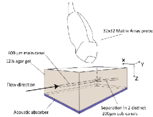
We manufactured a bifurcation inside tissue mimicking agar of width and height similar to the imaging wavelength (171 µm). 12% in weight of agar powder were mixed with degassed water at a temperature of 25 °C. We then proceeded to heat this solution by 20 °C steps with a microwave, stirring it in between cycles. The maximum temperature reached was above 80 °C to melt the agar powder with water. Afterwards, we proceeded to pour the gel in a box around the imprints of the bifurcation. These imprints were made of two nylon strings of 200 µm glued together and then separating into two separate strings. The glue made the main canal slightly larger than 400µm. This negative mold was removed after the gel solidified to allow the microbubble/water solution to flow through.
The micro-canal’s inlet was hooked up to a syringe whose flowrate was controlled by a syringe pump (Harvard Apparatus ® PHD 2000 Infusion). The flow rate used was 1ml/min. SonoVue ® microbubbles (Bracco S.p.A, Milan, Italy) ultrasound contrast agent was reconstituted following the manufacturer guidelines. The concentration in microbubbles of such a solution is [1-5] x 108
microbubbles per mL [30]. This solution was then mixed with water to obtain the desired range of concentrations
VSonovue/Vwater= [1/10000; 1/5000; 1/3000; 1/2000; 1/1000;
1/800; 1/600; 1/400; 1/200; 1/100]. In number of microbubbles per mL, this range covers [1-5] x [103-106]
microbubbles per mL. For each infusion, we acquired 500 volumes at a volume-rate of 500 Hz with pauses between imaging blocks to allow for data transfer. These pauses took most of the time : 89 s for transfer after 1 second of acquisition.
C. Beamforming and localization process
Delay-and-sum beamforming [Provost et al, 2014] was done a posteriori on a computer equipped with an Intel ® Xeon Haswell 10-core @ 2.60 GHz, 128 GB of RAM and a NVIDIA ® Tesla ® K40 GPU with 12Go of RAM. To reconstruct each voxel, the conventional delay and sum beamforming was applied to every element of the 2D array, thus making it a 3D DAS beamforming. The process was performed using Matlab 2017b with CUDA
Fig 1. Experimental setup : schematics of the agar gel containing the wall-less bifurcating canals
4
implementation (Mathworks Inc. Cambridge MA, USA). Each block (500 volumes), was beamformed at half wavelength in all directions. It took 45 seconds for each block including saving time. The same computer was used to implement the localization algorithm.Additional filtering was needed to prepare the images for localization. The time averaged intensity of each block was substracted from volume data to remove non or slow moving structures from the image. In high concentration cases, a clutter filter based on Singular Value Decomposition was implemented to better decorrelate moving and non-moving structures [[31], [7], [15]]. The agar gel fabricated as stated in II.B. still contains air trapped in microholes and thus scatters signal with similar intensity as the microbubbles. This makes it impossible to distinguish the bifurcation from the agar gel on non-filtered beamformed images. To locate the bifurcation we implemented a simple pre-processing technique where we sum all filtered images of one continuous sequence and divide it by the temporal maximum intensity of each pixel as follows 𝐼′(𝑧, 𝑥, 𝑦) =∑ 𝐼𝑓𝑖𝑙𝑡(𝑧,𝑥,𝑦,𝑖) 𝑁 𝑖𝑚𝑎𝑔𝑒𝑠 𝑖=1 max 𝑖 (𝐼𝑓𝑖𝑙𝑡(𝑧,𝑥,𝑦,𝑖)) (2)
This fast and simple technique allows to visualize areas where high temporal intensity gradients are located and thus the bifurcation. If the signal of a voxel is relatively constant through time, the filtered voxel will output a value close to 1. If the signal of the voxel contains one maximum, the filtered voxel will also output a value close to 1 however if the voxel contains many maxima as would be the case for a voxel through which many microbubbles are passing, the filtered voxel will output a value greater than 1 and close to the number of times a microbubble is passing through. This filter is computationally inexpensive and will reduce the memory required to visualize data as it frees itself from the 4th dimension (i.e. time). We then focused on these areas to do the 3D ULM.
After locating the bifurcation, we implemented two filters depending on the concentraion on original beamformed images to filter out phantom signal for each volume and retain microbubble signal only. 3D ULM was then applied to these images.
The localization process used here is based on QuickPALM [26] and has been entirely re-implemented to fit 3D data processing in Matlab. This new method determines the center of mass of the low-resolved bubble through its intensity profile: the ratio of the intensities of the pixels surrounding the local maximum over the intensity of the maximum defines the shift of the center of mass towards one direction. Analyzing this shift and fitting a model for the point spread function on a grid with higher
resolution yields the microbubble’s center position in the super-resolved basis.
The local maxima were computed for each volume of each sequence in a parallelized manner. This yielded (z,x,y) triplets, along with time, corresponding to the position of particles. A first filter based on the intensity of the local maximum detected was implemented, assuming that only the maxima with high intensity correspond to microbubbles. An additional filter based on the convolution between the localized microbubble signal and a simulated microbubble was also implemented. We simulated the PSF of the microbubble with an ellipsoid model of a minor axis size of 2*FWHM_Z (Full Width at Half Maximum in the Z dimension of a microbubble), and two equal large axis of 2*FWHM_X/FWHM_Y (Full Width at Half Maximum in the X/Y dimension of a microbubble). The FWHMs were estimated by measuring the beamformed signals of 20 microbubbles and were FWHM_Z=3 pixels, FWHM_X=FWHM_Y=5 pixels. The intensity of the microbubble is considered to be Gaussian distributed and the minimal acceptable value of the normalized 3 dimensional convolution is taken to be 0.6. This threshold was established, based on the inspection of detectable microbubbles on the images, as a tradeoff between the exclusion of noise points and the inclusion of microbubbles. The center of each of these microbubbles were calculated with the method explained above and this was registered as a new triplet (zcom,xcom,ycom). For a
sequence, this yields a matrix containing triplets of coordinates (x,y,z,t) corresponding to the positions of microbubbles in the 3 dimensional basis and time without modifying the original volume or reconstructing the full super-resolved volumes.
D. Tracking and velocimetry processing
After microbubbles positions are measured and stored, a tracking algorithm was implemented based on the Hungarian method or Kuhn-Munkres algorithm for assignment [27]. For each particle, the square distance to all of the particles in the subsequent frame is computed. We obtain a vector containing Nparticles(t+dt), the number of
particles in the frame (t+dt). In total, for each frame, we will obtain a matrix of size Nparticles(t)*Nparticles(t+dt). By
applying the Kuhn-Munkres algorithm, we are able to find the optimal pairing for the subsequent frames by minimizing the total squared distance. The Kuhn-Munkres algorithm allows considerable gain of time as its time complexity has been proven to be O(n3) [32]. This
algorithm is then looped on every frame. One advantage of this method is that it supports partial assignment (i.e. it will not pair a microbubble if there is no good candidate). We also studied the possibility of crossing trajectories: when two microbubbles cross path, they reach a certain position where they are next to each other. In a crossing
5
vessel scenario we have 4 points A(t), A(t+dt), B(t), B(t+dt). If the Euclidian distance between two points is minimized for A regardless of the minimization for B, there are cases where d(A(t),B(t+dt))<d(A(t),A(t+dt)) andd(B(t),B(t+dt))<d(B(t),A(t+dt)). However for our
algorithm this is not authorized as the pairing should be unique. Using the direction information from the trajectories, it is also possible to exclude crossing trajectories. A rejection filter is then applied to the microbubble position registered to eliminate microbubbles which do not follow long enough tracks : tracks smaller than 15 frames – 30 ms – are considered invalid. This threshold is justified by the fact that in a 3D volume, we should be able to reconstruct the tracks of the microbubble as long as they stay in the field of view which is considerably larger than the microcanal transverse axis. If a track is less than 30 ms, it could come from either noisy signals, or from incomplete tracking of a microbubble because of a pairing failure. In any case, a track of 30 ms contains a small enough amount of information to be dispensed with.
Thanks to the trajectories, it was possible to deduce the mean path of the canals. By looking at the distribution of the trajectories in each section, we can deduce the limits of the canals and the center. The mean path is defined as the streamline going from beginning to end of the field of view that is exactly centered in each direction (z,x,y) with respect to the walls of the canal.
The tracks are then used to compute velocity measurement based on the compounded volume rate in three dimensions using a differentiate method without interpolation. Each particle has its velocity computed through its trajectory and according to its temporal sampling. This follows the traditional Lagrangian approach to calculate velocity fields as demonstrated experimentally in [33]. The accuracy of these velocities is thus influenced by the accuracy of both particle assignment and the tracking algorithm.
It was also possible to calculate the average velocity in the canals based on the flowrate of the syringe pump and the diameters obtained in this section. With conservation of flow rate (1mL/min) and without taking into account pressure loss, the average velocity in the main canal is 79 mm/s which assuming the flow is laminar (Vmoy0.5*Vmax)
and gives a maximum velocity of 158 mm/s.
s mm D D Q S Q V lmain Lmain main main 79 / 2 * 2 * (3)
If we assume conservation of flow rate in the bifurcation we can write: ) * ( * ) * ( * ) * ( * lright Lright right lleft Lleft left lmain Lmain main right left main D D V D D V D D V Q Q Q (4) where DLand Dlare respectively the large diameter and the small diameter for the canals.
In addition to velocimetry, the trajectories were interpolated with a spline model to achieve better spatial sampling of the bifurcation. The original points given by the trajectories served as knots to construct the break sequence according to the centripetal scheme [34], by using the cscvn function packaged by Matlab. For each trajectory 1 million points were calculated on its respective spline and were then resampled to obtain a uniform spatial sampling of 1 µm in all three directions. We then projected all points belonging to a section of thickness 10 µm in the Y direction. By calculating the distance between the two closest points belonging to each side canals, we can estimate a separability criterion. This measure was repeated for sections going from main to side canals.
III. RESULTS
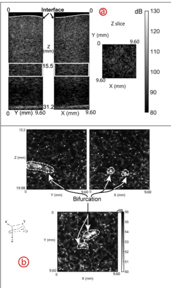
Figure 2 presents conventional beamformed images and images after filtering. A voxel in our images measures 84.5µm x 150µm x 150 µm and so the ratio of all the subsequent figures is kept according to this dimension. Figure 2a shows three slices: parallel to the main axis of the bifurcation and orthogonal to the probe plane (z,x); perpendicular to the main axis of the bifurcation and orthogonal to the probe plane (z,y); and parallel to the plane of the probe (x,y). A basis (z,x,y), was placed over the images in figure 1 and will be used in the following sections. To improve readability, the new images deduced by the way of the pre-processing were focused on the region of interest. These images are presented in figure 2b. Because microbubbles appear sporadically throughout the experiment, we can locate the bifurcation by the pre-processing technique. However this does not allow to extract the microbubbles independently and track their journey due to temporal averaging. The representation of the bifurcation with this process is blurred and does not allow accurate measurement of its dimensions.
After locating the bifurcation, two different processing techniques were implemented to enhance the microbubble
6
to agar signal ratio depending on the microbubble concentration. To visualize microbubbles in concentrations lower than 1/5000th of the Sonovue ® vial solution, thetime averaged over a continuous sequence of 1 second was calculated and subtracted from each image. This approach benefits from a straightforward decoupling between agar background signals and microbubbles signature regardless of their velocities. However, for higher concentration, we found that this temporal averaging process, while sufficient to remove agar gel signal, also modified adjacent microbubble signals thus impeding localization. The reason why this happens is that when microbubbles are near one another (as is the case in high concentration), their signals interfere together during the temporal averaging and rather than maximizing only the agar’s intensity, the filter also produces high intensities where microbubbles are cluttered together. In that case, subtracting the time average to each image removes cluttered microbubbles’ signal. Rather than using this filter that is based on intensity
over time, we decided to use the singular value decomposition (SVD). Because SVD has been proven to be able to decorrelate tissue, blood and microbubbles based on their spatiotemporal signature [31], [7], it is less sensitive to high concentration or microbubble cluttering. This SVD filter worked by removing the first few most energetic eigenvalues in the singular value decomposition. Depending on the concentration, either the [30,20,15] most energetic eigenvalues were removed because they represent highly spatio-temporal coherent signal. The higher the concentration, the less eigenvalues were discarded. The images for low concentration obtained are shown in figure 3 a, b. The red crosses pinpoint where microbubbles are.
The triplets (zcom,xcom,ycom) obtained in the methods section
are plotted in a 3 dimensional space to reveal the bifurcation in the super-resolved basis (figure 4 left column). These triplets are defined for each volume through the entire duration of acquisition. On figure 4, we plotted the particles localized in a super-resolved basis for two different concentrations using 2000 successive volumes (4 seconds). Pre-tracking, the number of microbubbles detected for low concentration is 5314, and Fig. 2: Typical slices of the 3D volume obtained after conventional
beamforming. Additional filtering by the pre-processing technique. This technique is a very simple way to locate areas with high concentration of microbubbles.
2.a) Single slices of the entire imaged voxel in 3 directions. The white squares indicate where the subsequent images (2.b) are taken. 2.b) Isometric slices at region of interest after pre-processing
Fig 3. Isolated microbubbles in different slices of the volumetric acquisition. Slices for 3 directions at two different times a) Frame taken at t=0. The particles detected through local maxima are outlined with a red cross. The coordinates of the red crosses have been drawn with dashed white lines.
b) In the same manner, the same slices of the subsequent frame (2 ms later) have been generated. In slice Y, only two particles were located. In this slice, only the cross section of the tubes are visible so only a limited amount of microbubbles will be detected. dB
7
29351 for high concentration. Post-tracking, the number of microbubbles detected for low concentration is 525, and 393 for high concentration.Microbubbles flow continuously in the canal and can be followed on ultrasound images as illustrated on figure 3. By implementing the 3D tracking process previously discussed on the center of the microbubbles, we recovered the independent trajectories of the localized microbubbles (figure 5). Each line is the trajectory of one microbubble. The colour of each line is encoded depending on the duration of the track. Most of the tracks follow the path of the canals and are relatively short in duration : the average track duration is 32 ms, with a standard deviation of 14 ms and the longest trajectory is 138 ms.
Fig. 5. Trajectories and scatter plot of microbubbles detected. a) Color represents the length of the vectors. b) Scatter plot of each center of microbubbles detected that can be tracked
Thanks to the additional information given by the directivity of the trajectory, we implemented a filter to keep the microbubbles following the main direction of the flow.
Positions obtained after this additional filter are plotted in figure 5.b. By doing these operations on all of the volumes acquired, it was possible to obtain a large number of microbubbles positions for 6000 volumes (n=288389 positions) which correspond to our final image.
MAIN CANALS SIDE CANALS
Fig 6. Slices of the main and side canals
a) Transverse cut of main canal (X,Z). Mean width of main canal was found to be 680 +/-5 µm after making 21 transverse cuts of thickness 75 µm with a standard deviation of 85 µm. Mean height of the main canal was found to be 396 +/- 1 µm after making 21 transverse cuts of thickness 75µm with a standard deviation 29µm.
Transverse cut of left and right canal (X,Z).
b) Mean width of left canal was found to be 460 +/- 5 µm after making 11 transverse cuts of thickness 300 µm with a standard deviation of 10 µm. Mean height of the left canal was found to be 237 +/- 1 µm after making 11 transverse cuts of thickness 300µm with a standard deviation of 24µm.
c) Mean width of right canal was found to be 310 +/- 5 µm after making 11 transverse cuts of thickness 300 µm with a standard deviation of 10 µm. Mean height of the right canal was found to be 226 +/-1 µm after making 11 transverse cuts of thickness 300µm with a standard deviation of 24µm.
Subsequent to the filter based on tracking, the velocimetry algorithm was applied to each triplet to yield 3D velocity maps in the bifurcation. The velocity components in the 3 directions give us access to the angles of the trajectories and thus the direction of the bifurcation. This in turn allows to locate the mean path by locating the center of each section and the angle of the trajectories. By having the direction of the bifurcation and the mean path, we can deduce the velocity profiles in the flow by defining a new basis centered on the mean path and with one of its vector colinear to the direction of the flow. This basis changes along the canals with their direction. After calculating each basis, we can cut profiles perfectly orthogonal to the main direction of the flow and thus have access to the section which will give the width and height of the canal. Such profiles are presented in figure 6. For each slice, the positions of the microbubbles are plotted with crosses and calculating the width and height of the canal is done by taking the farthest positions in each direction.
PRE TRACKING POST TRACKING
C o n ce n tr atio n = 1 /1 0 0 0 0 C o n ce n tr atio n = 1 /8 0 0
Figure 4. Cumulated scatter plot of each centre of microbubbles detected for different concentrations pre and post-tracking 4. (a,c) are without tracking and 4.(b,d) are exploiting tracking algorithm. The concentration used are 1/10000 for (a,b) and 1/800 for (c,d).
8
Each time we applied the localization algorithm, we noted the number of microbubbles detected. Values are reported in table 1. Sometimes, the tracking algorithm implemented failed to pair the microbubbles, in particular at higher concentrations. The main resulting consequence was that the trajectories were too short or went in a direction incoherent with the direction of the flow. We assessed this by looking at the direction uniformity of each tracks compared to the supposed direction of the flow and to the average length of a track. We looked at the direction directly on the reconstructed images and we measured the standard deviation of the tracks over a sequence to assess the ability to track. This was labeled in table 1 as an inability to track.Concentration Number of microbubbles
per frame Ability to track 1/10000 67 +/- 8 Yes 1/5000 68 +/- 7 Yes 1/3000 10 +/- 1 Yes 1/2000 10 +/- 1 No 1/1000 10 +/- 1 No 1/800 4.9 +/- 0.1 No 1/600 0 No 1/400 0 No 1/200 0 No 1/100 0 No
Table 1. Table giving the number of particles and the ability to track them
As we obtained profiles perfectly orthogonal to the main direction of the flow, it is possible to look at the velocity components of the microbubbles present in these profiles and obtain an instantaneous velocity profile at each cut. The velocity profiles averaged for several transverse slices (X,Z) are realigned and plotted over the bifurcation in figure 7. The positions of the microbubbles localized in the canals are also plotted as black dots. The walls of the canals were drawn by hand trying to pass through the maximum number of particles with minimal deviation. It was possible to do this in the other direction (Y,Z) and yielded additional velocity profiles presented in figure 7b.
In our case, we measured a maximum velocity of 144 mm/s +/- 3.6mm/s (standard deviation as described in the
Methods section). The difference between the
experimental value and the one calculated with conservation of flow rate can be explained by the fact that we do not take into account pressure loss.
Experimentally, the diameters were found to be smaller in the right side canal and the velocities higher which is confirmed by the equation (4). If we assume all of the flow goes into one of either canal, we obtain using the same equation (3) as for calculating main velocity, Vleft= 195
mm/s, Vright= 298 mm/s.
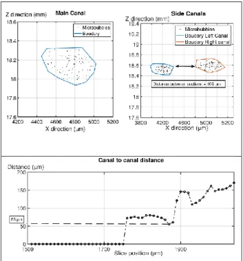
After applying the cubic spline based spatial resampling describe in the Methods section, we were able to produce figures similar to figure 6. but with resampled data – allowing us to reach higher definition of the canals sides. The microbubbles positions plotted in figure 8.a) and 8.b) belong to two slices of 10 µm in the Y direction. They were taken respectively at y=1310 µm and y=3600 µm (y=0 µm being the edge of the probe). The boundaries were automatically defined using the boundary function in Matlab. Such graphs were plotted for 54 consecutive slices ranging from y=1500 µm to y= 2040 µm and the distance between two points belonging to each side canal was recorded. When such points could not be found, the distance was noted to be 0. The distances measured are plotted on figure 8.c). The minimal distance measured between two distinct microbubbles was 55 µm.
Figure 8. Slices of main and side canals with cubic spline resampling and separability criterion
a) Two 10 µm slices representing main and side canals after cubic spline resampling
b) Distances between boundaries of the side canals measured
XZ Plane YZ Plane
Figure 7. Velocity profiles in two orthogonal slices
a) Velocity profiles in bifurcation (X,Z) axis. Maximum velocity is 144 mm/s +/- 3.6mm/s. Dashed lines represent the profile orthogonal to the microcanals based on the direction of the streamlines. b) Velocity profiles in bifurcation (Y,Z) axis. As the two canals are overlapped, the velocity profiles are shifted in this representation.
9
IV. DISCUSSION
In this study we introduced and demonstrated the possibility to use 4D ultrafast ultrasound scanners to implement volumetric ultrafast Ultrasound Localization Microscopy. We developed an in-vitro setup that allowed us to image flow in three dimensions and implemented a 3D algorithm for localization, tracking and velocimetry of microbubbles at subwavelength resolution.
To demonstrate super-resolution, we observed the passage of microbubbles in channels at the scale of the wavelength. As the resolution is defined by the smallest structures that can be separated in an image, the easiest way to confirm ULM is to look at small structures close to each other. For this, we modified previously described microvessel phantoms [[4], [9]] to obtain easy to manufacture Y-shaped channels that can be oriented in three directions. A syringe pump allowed a controlled flow rate to compare the ULM velocimetry with expected maximum microbubble velocities.
The intensity on beamformed volumes highlighted the vessels into which microbubbles were flowing. Thanks to the absence of movement of the phantom, clutter filtering could be performed with a simple subtraction of the mean signal for low concentrations. However for higher concentrations, we used the singular value decomposition filter [[31], [7], [15]]. This filter has the ability to distinguish microbubbles and agar based on their spatiotemporal signature and is less sensitive to concentration than conventional temporal averaging filter but puts additional complexity to the post-processing and lacks the ability to distinguish slow moving microbubbles. Usually, tissue signal is concentrated in high singular values because its dynamics are slower than average microbubble movement and noise. However, for slow moving microbubbles in small microvasculature, this is no longer true and removing large singular values actually removes some of the slow moving microbubbles. The implemented filter and the SVD threshold are thus a compromise between microbubble specificity and sensitivity. In our case, the thresholds were chosen empirically to improve the quality of the image enough to be able to see microbubbles moving in the tube while keeping these thresholds to a minimum to avoid losing
microbubbles. Adaptative filtering, as described by
Baranger et al. [35], could also be explored. For in vivo
experiment, the dose of Sonovue commonly used
[[7], [10], [13]] lead to a high concentration of microbubbles in the blood. We predict that similarly to 2D ULM, SVD based filtering will be preferred to the temporal averaging filter for 3D ULM.
An additional challenge was to have sufficient signal-to-noise ratio to be able to implement ULM while limiting the amount of energy transmitted to each microbubble to prevent destruction. This leads to our selection of
peak-negative-pressures around 300 kPa. Along with acoustic pressure, hydrostatic pressure in small channels could also have led to microbubble disruption. However, according to [35] there is less than 3% destruction of microbubble with a 27 gauge syringe (400µm diameter), 0.1 ml/sec. Since we have a maximum flow rate inside canals of 0.016 ml/s, we conclude that we have no microbubble destruction due to hydrostatic pressure.
In [7], a method to localize the center of the microbubble with an interpolation of the desired super-resolution factor was proposed. While this allows to work directly on beamformed images, the interpolation method is costly both in time and processing power for 2D analysis. For 3D, it becomes unmanageable as the data interpolated by a factor of 10 sees its size increase by a factor of 1000. Interpolating one volume of 11.9 MBytes (0.2 second), would yield 11.9 GBytes of additional data. As we are required to do the uULM process on thousands of volumes, this technique becomes rapidly memory expensive. A novel localization technique was thus implemented. This technique while being more manageable also proves to be considerably faster (we calculated in 2D that for 75000 frames, the interpolation approach takes 12hours 30 minutes on a high performance 4 cores processor PC, Intel i7-6700 at 3.4GHz and a NVIDIA GeForce GTX1080, while the weighted average method takes only 2 minutes 40s).
The original QuickPALM algorithm is coded in Java for the ImageJ platform [37]. It is readily usable for 2D images if you choose to work with images in a graphical format. As we choose to work with beamformed data we could also work with images but we would lose the information of phase present in the IQs. We ported the QuickPALM algorithm from Java to Matlab in 2D at first and then extended it into three dimensions. The drift correction filter based on fiduciary landmarks was abandoned in our method because the in vitro technique is not subject to motion and also because no fiduciary landmarks were present in the gel. We worked in Matlab to make this code as fast as possible using parallelization of the mathematical operations to take advantage of multiple cores CPUs, and we added the convolution step mentioned above. We decided to use the method based on the calculation of the center of mass of the low-resolved bubble through its intensity profile. It is a straightforward method that minimizes computational requirements and do not need to interpolate the data. Sage et al [38] recently published an extensive paper about the different techniques available to perform Single Molecule Localization Microscopy and rated the different algorithms. As we want to lower computational cost as much as possible and have an easy to package tool, it seems that QuickPALM is a good candidate for translation to 3D ULM.
10
The new localization process was implemented on each volume. As pictured on figure 4, the higher the concentration, the more particles are detected pre-tracking for the same acquisition duration. This means that higher concentration of microbubbles lead to faster reconstruction of the canals. The high concentration of microbubbles makes it very easy to distinguish the bifurcation compared to the tissue surroundings but requires a less discriminative tissue/bubble filtering to cope with microbubble cluttering. However after tracking, a lot of microbubbles detected are filtered out because the tracking is unable to perform well. The high concentration of microbubbles and possible cluttering makes tracking the same microbubble through the bifurcation more difficult. This is because, in the case of high concentration, microbubble signals are so close to each other, that the Munkres assignment can not assign microbubbles to one another. In terms of algorithm, it is the minimization step of the cost matrix that poses problem. Having so many particles means that the minima found after the Kuhn-Munkres algorithm are not unique. Less particles are detected and whole areas of the canals are missing. In both concentrations, the tracking algorithm correctly removes false detections in tissue which greatly improves the quality of the image. The trade-off is similar to that between Particle Image Velocimetry (PIV) where concentrations of tracers are high and thus do not allow individual tracking and Particle Tracking Velocimetry (PTV), where concentrations of tracers are low and allow tracking but take longer to do velocimetry [28]. PTV allows individual tracking but is more difficult and takes longer to implement. In our case, if the concentration is further increased, the Rayleigh criterion of separation in between microbubbles will not apply anymore and will lower the number of microbubbles taken in each frame. A new algorithm should be implemented to separate close microbubbles in this case. These phenomena illustrate the importance of concentration on localization.The number of microbubbles counted gives us information about the efficiency of the algorithm but cannot be correlated with the real number of microbubbles. This shortcoming is due to the fact that we cannot know the exact number of microbubbles we inject because the concentration of the microbubbles in a Sonovue vial varies by a factor as much as 5 [30]. It would be useful to know how many microbubbles we actually inject to assess the quality of our algorithm and we could do that by using another means of visualizing them such as a microscope and coating the microbubbles in fluorescent material. This measurement could be performed with a Coulter counter before injection or fluorescent microscopy in the measurement chamber itself.
The tracking algorithm allowed us to implement velocimetry and yielded geometric information about the channels like their mean paths, angles and their profiles along each axis. The information is accessible even with a
low number of detected microbubbles as only a dozen of velocity vectors were sufficient to measure the angle of the flow. It is important to note that these velocity profiles were obtained in vessels the size of the wavelength, demonstrating that ULM can provide super-resolution both for microbubble densities and velocities. This opens up the way towards fast basis projection to determine mean path and streamlines in 3 dimensions, as well as, easy tortuosity measurement in microvasculature.
The trajectories after localization were relatively short (a few dozens of ms) compared to the time of one acquisition. Theoretically the longest trajectory could be 1 s as each acquisition lasts 1 s, however, this would be the case only if the velocity of the microbubble was below 10 mm/s. The average velocity in the main canal being around 79 mm/s, most of the microbubbles leave the observed volume in much less than 1 second. In vivo, for these vessel diameter, we expect slower flow, which would facilitate tracking at these compounded volume rates.
The width of the canals measured on the super-resolved image are larger than their height. It is hypothesized that this is due to agar collapsing on itself when it is molded over the nylon strings. These features were verified by cutting slices of the agar gel and observing them with a microscope (Leica DMIL LED FLUO). Overall, the minimum height was close to the imaging wavelength (226 µm for the right side canal to be compared with a wavelength of 171 µm) and the B mode resolution (lambda*f/D=1.6*lambda=276 µm). We are able to measure such distances because the precision of our localization algorithm yields images with a resolution enhanced with respect to the B-mode resolution. However the resolution for ULM is not only the localization precision but also depends on the number of particles accumulated.
Spatial resampling has been documented in the field of Particle Tracking Velocimetry [[39], [40]] where the need for high spatial sampling in 3D is a problem for Lagrangian flow measurement. Drawing from this, we turned to cubic spline interpolation to reconstruct trajectories. This scheme achieves smoother tracks than the linear interpolation scheme and supports continuity at the breakpoints which ensures continuity on speed and acceleration. This process performed in the final stage of the ULM framework allowed us to reach higher spatial sampling of the bifurcation and so resulted in a denser representation of the canals. Thanks to this denser representation, we were able to have sufficient particle positions in 10 µm thick slices to be able to distinguish the canals branching out with a resolution of 55 µm. With that measurement and velocimetry we have retrieved 3 dimensional information with precision much smaller than the diffraction limit in all dimensions. Our resampling could be further improved by using other schemes or we could dispense of it if we
11
acquire with higher volume-rate but this poses problems of data overload. Moreover the measurement of 55 µm represents a higher limit on the resolution we can reach because it largely depends on the probability of a microbubble running along the edge of the canal. This probability is linked to velocity profile - as low velocity areas have less renewal rate and so less microbubbles present throughout the acquisition - and also to the concentration of microbubble. As there is a constraint on the maximum concentration allowing ULM, it is likely that the solution would be to acquire longer to get a more complete seeding of the canals. The scheme developed here is likely to be useful to further improve the velocimetry in areas where microbubble counts are low invivo.
An advantage of the volumetric ULM process is the sparsity degree of super-resolved images. As this degree is high, it is useful to compute and save the positions of the microbubbles through the algorithm. This technique allows to manipulate smaller dataset: a 1 second acquisition is about 23 GBytes for volumetric images (Radiofrequency and beamformed images) alone whereas a matrix containing intensities, positions of the microbubbles weighs only 800 kBytes. After filtering the positions by tracking, this scales down to 75 kBytes. This represents a compression factor of about 300 000. In a case where the uULM algorithm would take around the same amount of time than the acquisition and beamforming of the data (as is already the case in 2D), it would save a considerable amount of space and could allow for faster visualization. Currently, volumetric ultrafast ULM retains some drawbacks. An important aspect is that the size of the data produced with 1024 channels limits the speed at which we can transfer the data from the ultrasound machine to the computer memory. This doesn’t restrict the framerate per se but limits the time between blocs of acquisitions thus increasing the overall experimental time and reducing the number of detected microbubbles. Another drawback is that this technique requires computational power which brings challenge to implement in a clinical setting. However this requirement will decrease in the coming years according to Moore’s law. The increase of computational power, as well as, performance in ultrasound systems will minimize such drawbacks and increase the interest for this technique.
Beyond computer processing limitations, a more important issue is the signal-to-noise ratio of the microbubble. Due to the size of the elements in 2D matrix-arrays, the SNR is often lower than with conventional 1D probes. Due to the element size, the sensitivity problem of 2D matrix arrays is common and is usually solved by driving the probe with a higher voltage. However this leads to an increase in the energy transmitted to the medium and the ISPTA and PNP values, bringing them close to the destruction threshold of
microbubbles. Because we would like to limit destruction of microbubbles, we deliberately chose a low voltage to drive the probe but increased the number of transmissions employed to produce an image. In the end, we found that a total of 4 titled angles with a f/D ratio of 1.6 enabled us to obtain sufficient image quality to localize microbubbles (SNR of bubbles is around 20 dB increase on filtered images). Thanks to the ultrafast capability of the electronic, transmitting such a number of angles still allowed us to achieve compounded volume rates up to 1000 Hz. We chose a volume rate of 500 Hz to limit data size. Fortunately, the experiment presented here faces no issue due to motion and the response of the tissue is easily filtered out.
The sensitivity problem is likely to be more important in-vivo. More transmissions would be required to obtain images of appropriate quality for localization. The problem with this is firstly that the compounded volume rate is lowered and secondly that the amount of data to transfer to make an image gets larger. The first problem can be solved for ULM of microvasculature as it was shown that high frame rates are not needed as microbubbles move slowly in small structures [16]. The second issue however is more important as the limitations come from the hardware capability of the system: 512 channels only in reception, SATA buses are limited to 6Gb/s, RAM available for each machine is 16 Gb. We hope that with the growing interest in 4D imaging, the quality of the probes and electronics will improve.
In general, we have achieved super-resolution imaging of a micro-vessel phantom in a full 3D volume using volumetric ultrafast ultrasound localization microscopy in a limited time. Not only does the measured size of the wavelength-scale vessels compare well with expectations and their separation can be defined with a resolution of tens of microns, but the microbubble velocimetry also correspond to predicted sub-wavelength flow patterns. The processes developed here to filter out microbubbles, track them and use the direction, length and velocity magnitude information drawn from the trajectories are already commonly used in 2D in vivo applications [[10], [11], [16]]. The related thresholds and parameters will have to be modified and adapted for each in vivo applications. Our attention is now turned towards application of this technique in vivo in small animal models, as it would allow us to answer many difficulties we face in 2D. In particular, plane-by-plane ULM acquisitions require several boluses or long infusion times to reconstruct an entire organ such as the rat brain. The volumetric ULM technique described in this paper would allow the observation of the majority of this organ volume in a single sequence. Also, the 3D vascular network in organs is currently badly represented by its 2D projection in planar ULM and requires, in the future, a full volumetric method. Moreover, appropriate
12
motion correction in-vivo requires information in the three dimensions. Future work includes the investigation of alternative options to reduce the number of electronic channels needed to acquire volumetric images.V.
CONCLUSION
Volumetric ultrafast Ultrasound Localization Microscopy delivers volumes with enhanced resolution in the three dimensions compared to conventional 3D B-mode imaging within acceptable acquisition times. Moreover, by tracking the microbubbles through time, it allows velocimetry to retrieve dynamics of the observed flows and to access geometric properties at the scale of the wavelength. In vitro feasibility was demonstrated but additional in vivo applications remain to be explored. Volumetric uULM could be a solution to the main limitations, encountered in planar ULM, such as microbubble tracking and motion correction related to the absence of elevation information.
ACKNOWLEDGEMENT
This work was supported principally by Agence Nationale de la Recherche, within the project ANR Tremplin Resolve Stroke. This work was supported by LABEX WIFI (Laboratory of Excellence ANR -10 -LABX -24) within the French Program “Investments for the Future” under reference ANR -10 - IDEX -0001 -02 PSL* . Thanks to Hicham Serroune for constant support and Laura Zamfirov, Kailiang Xu for insightful discussions.
REFERENCES
[1] Olivier Couture, Mickael Tanter, et Mathias Fink,
« Patent 889 Cooperation Treaty
(PCT)/FR2011/052810 ».
[2] O. Couture, B. Besson, G. Montaldo, M. Fink, et M. Tanter, « Microbubble ultrasound super-localization imaging (MUSLI) », 2011, p. 1285‑1287.
[3] E. Betzig et al., « Imaging Intracellular Fluorescent Proteins at Nanometer Resolution », Science, vol. 313, no
5793, p. 1642‑1645, sept. 2006.
[4] Y. Desailly, O. Couture, M. Fink, et M. Tanter, « Sono-activated ultrasound localization microscopy », Appl.
Phys. Lett., vol. 103, no 17, p. 174107, oct. 2013.
[5] M. A. OˈReilly et K. Hynynen, « A super-resolution ultrasound method for brain vascular mapping: Super-resolution ultrasound method for brain vascular mapping », Med. Phys., vol. 40, no 11, p. 110701, oct.
2013.
[6] O. M. Viessmann, R. J. Eckersley, K. Christensen-Jeffries, M. X. Tang, et C. Dunsby, « Acoustic super-resolution with ultrasound and microbubbles », Phys.
Med. Biol., vol. 58, no 18, p. 6447‑6458, sept. 2013.
[7] C. Errico et al., « Ultrafast ultrasound localization microscopy for deep super-resolution vascular imaging »,
Nature, vol. 527, no 7579, p. 499‑502, nov. 2015.
[8] V. Hingot, C. Errico, M. Tanter, et O. Couture, « Subwavelength motion-correction for ultrafast Ultrasound Localization Microscopy », 2017, p. 1‑1. [9] K. Christensen-Jeffries et M. Tang, « 3-D In Vitro
Acoustic Super-Resolution and Super-Resolved Velocity Mapping Using Microbubbles », p. 9.
[10] J. Foiret, H. Zhang, T. Ilovitsh, L. Mahakian, S. Tam, et K. W. Ferrara, « Ultrasound localization microscopy to
image and assess microvasculature in a rat kidney », Sci.
Rep., vol. 7, no 1, déc. 2017.
[11] P. Song et al., « Improved Super-Resolution Ultrasound Microvessel Imaging With Spatiotemporal Nonlocal Means Filtering and Bipartite Graph-Based Microbubble Tracking », IEEE Trans. Ultrason. Ferroelectr. Freq.
Control, vol. 65, no 2, p. 149‑167, févr. 2018.
[12] F. Lin, S. E. Shelton, D. Espíndola, J. D. Rojas, G. Pinton, et P. A. Dayton, « 3-D Ultrasound Localization Microscopy for Identifying Microvascular Morphology Features of Tumor Angiogenesis at a Resolution Beyond the Diffraction Limit of Conventional Ultrasound »,
Theranostics, vol. 7, no 1, p. 196‑204, 2017.
[13] O. Couture, V. Hingot, B. Heiles, P. Muleki-Seya, et M. Tanter, « Ultrasound localization microscopy and super-resolution: a state-of-the-art », IEEE Trans. Ultrason.
Ferroelectr. Freq. Control, p. 1‑1, 2018.
[14] M. Tanter et M. Fink, « Ultrafast imaging in biomedical ultrasound », IEEE Trans. Ultrason. Ferroelectr. Freq.
Control, vol. 61, no 1, p. 102‑119, janv. 2014.
[15] Y. Desailly, J. Pierre, O. Couture, et M. Tanter, « Resolution limits of ultrafast ultrasound localization microscopy », Phys. Med. Biol., vol. 60, no 22, p.
8723‑8740, nov. 2015.
[16] Hingot, Vincent, Errico, Claudia, Heiles, Baptiste, Rahal, Line, Tanter, Mickael, et Couture, Olivier, « Microvascular flow dictates the compromise between spatial resolution and acquisition time in ultrasound localization microscopy », 2018.
[17] Olaf T. von Ramm, Stephen W. Smith, et Henry G. Pavy Jr., « High-speed Ultrasound Volumetric Imaging System- Part II: Parallel Processing and Image Display ». IEEE T UFFC, 1991.
[18] G. R. Lockwood, J. R. Talman, et S. S. Brunke, « Real-time 3-D ultrasound imaging using sparse synthetic aperture beamforming », IEEE Trans. Ultrason. Ferroelectr. Freq. Control, vol. 45, no 4, p. 980‑988, juill.
1998.
[19] C. R. Hazard et G. R. Lockwood, « Theoretical Assessment of a Synthetic Aperture Bearnforrner for Real-Time 3-D Imaging », p. 9.
[20] J. A. Jensen et al., « SARUS: A synthetic aperture real-time ultrasound system », IEEE Trans. Ultrason.
Ferroelectr. Freq. Control, vol. 60, no 9, p. 1838‑1852,
sept. 2013.
[21] J. Provost et al., « 3D ultrafast ultrasound imaging in
vivo », Phys. Med. Biol., vol. 59, no 19, p. L1‑L13, oct.
2014.
[22] J. Provost, C. Papadacci, C. Demene, J.-L. Gennisson, M. Tanter, et M. Pernot, « 3-D Ultrafast Doppler Imaging Applied to the Noninvasive and Quantitative Imaging of Blood Vessels in Vivo », p. 12, 2016.
[23] S. Holbek, T. L. Christiansen, M. F. Rasmussen, M. B. Stuart, E. V. Thomasen, et J. A. Jensen, « 3-D vector velocity estimation with row-column addressed arrays », 2015, p. 1‑4.
[24] M. Correia, J. Provost, M. Tanter, et M. Pernot, « 4D ultrafast ultrasound flow imaging: in vivo quantification of arterial volumetric flow rate in a single heartbeat »,
Phys. Med. Biol., vol. 61, no 23, p. L48‑L61, déc. 2016.
[25] J. Gennisson et al., « 4-D Ultrafast Shear-Wave Imaging », IEEE Trans. Ultrason. Ferroelectr. Freq.
Control, vol. 62, no 6, p. 1059‑1065, juin 2015.
[26] R. Henriques, M. Lelek, E. F. Fornasiero, F. Valtorta, C. Zimmer, et M. M. Mhlanga, « QuickPALM: 3D real-time photoactivation nanoscopy image processing in ImageJ »,
Nat. Methods, vol. 7, no 5, p. 339‑340, mai 2010.
[27] H. W. Kuhn, « The Hungarian method for the assignment problem », Nav. Res. Logist. Q., vol. 2, no 1‑2, p. 83‑97,
mars 1955.
[28] F. Bourgeois et J.-C. Lassalle, « An extension of the Munkres algorithm for the assignment problem to rectangular matrices », Commun. ACM, vol. 14, no 12, p.
13
[29] O. Casula et D. Royer, « Visualisation des champs ultrasonores par interférométrie hétérodyne », J. Phys. IV, vol. 04, no C5, p. C5-1217-C5-1220, mai 1994.
[30] M. Schneider, « Characteristics of SonoVueTM »,
Echocardiography, vol. 16, no s1, p. 743‑746, oct. 1999.
[31] C. Demene et al., « Spatiotemporal Clutter Filtering of Ultrafast Ultrasound Data Highly Increases Doppler and fUltrasound Sensitivity », IEEE Trans. Med. Imaging, vol. 34, no 11, p. 2271‑2285, nov. 2015.
[32] J. EDMONDS, « Theoretical Improvements in Algorithmic Efficiency for Network Flow Problems », p. 17.
[33] V. Bondur, Y. Grebenyuk, E. Ezhova, A. Kandaurov, D. Sergeev, et Y. Troitskaya, « Applying of PIV/PTV Methods for Physical Modeling of the Turbulent Buoyant Jets in a Stratified Fluid », p. 23.
[34] E. T. Y. Lee, “, « Choosing nodes in parametric curve interpolation », Comput.-Aided Des., vol. 21, no 6, p. 363–
370, juill. 1989.
[35] J. Baranger, B. Arnal, F. Perren, O. Baud, M. Tanter, et C. Demene, « Adaptive Spatiotemporal SVD Clutter Filtering for Ultrafast Doppler Imaging Using Similarity of Spatial Singular Vectors », IEEE Trans. Med. Imaging, vol. 37, no 7, p. 1574‑1586, juill. 2018.
[36] E. Talu, R. L. Powell, M. L. Longo, et P. A. Dayton, « Needle Size and Injection Rate Impact Microbubble Contrast Agent Population », Ultrasound Med. Biol., vol. 34, no 7, p. 1182‑1185, juill. 2008.
[37] C. A. Schneider, W. S. Rasband, et K. W. Eliceiri, « NIH Image to ImageJ: 25 years of image analysis », Nat.
Methods, vol. 9, no 7, p. 671‑675, juill. 2012.
[38] D. Sage et al., « 1 Super-resolution fight club: A broad assessment of 2D & 3D 2 single-molecule localization microscopy software », p. 25.
[39] B. Lüthi, A. Tsinober, et W. Kinzelbach, « Lagrangian measurement of vorticity dynamics in turbulent flow », J.
Fluid Mech., vol. 528, p. 87‑118, avr. 2005.
[40] K. Hoyer, M. Holzner, B. Lüthi, M. Guala, A. Liberzon, et W. Kinzelbach, « 3D scanning particle tracking velocimetry », Exp. Fluids, vol. 39, no 5, p. 923‑934, nov.