HAL Id: hal-02079820
https://hal.archives-ouvertes.fr/hal-02079820v2
Preprint submitted on 17 Apr 2019
HAL is a multi-disciplinary open access
archive for the deposit and dissemination of
sci-entific research documents, whether they are
pub-lished or not. The documents may come from
teaching and research institutions in France or
abroad, or from public or private research centers.
L’archive ouverte pluridisciplinaire HAL, est
destinée au dépôt et à la diffusion de documents
scientifiques de niveau recherche, publiés ou non,
émanant des établissements d’enseignement et de
recherche français ou étrangers, des laboratoires
publics ou privés.
Riemannian geometry learning for disease progression
modelling
Maxime Louis, Raphäel Couronné, Igor Koval, Benjamin Charlier, Stanley
Durrleman
To cite this version:
Maxime Louis, Raphäel Couronné, Igor Koval, Benjamin Charlier, Stanley Durrleman. Riemannian
geometry learning for disease progression modelling. 2019. �hal-02079820v2�
progression modelling
Maxime Louis1,2, Rapha¨el Couronn´e1,2, Igor Koval1,2, Benjamin Charlier1,3,
and Stanley Durrleman1,2
1 Sorbonne Universit´es, UPMC Univ Paris 06, Inserm, CNRS, Institut du cerveau et
de la moelle (ICM)
2 Inria Paris, Aramis project-team, 75013, Paris, France
3
Institut Montpelli`erain Alexander Grothendieck, CNRS, Univ. Montpellier
Abstract. The analysis of longitudinal trajectories is a longstanding problem in medical imaging which is often tackled in the context of Riemannian geometry: the set of observations is assumed to lie on an a priori known Riemannian manifold. When dealing with high-dimensional or complex data, it is in general not possible to design a Riemannian geometry of relevance. In this paper, we perform Riemannian manifold learning in association with the statistical task of longitudinal trajectory analysis. After inference, we obtain both a submanifold of observations and a Riemannian metric so that the observed progressions are geodesics. This is achieved using a deep generative network, which maps trajectories in a low-dimensional Euclidean space to the observation space.
Keywords: Riemannian geometry · Longitudinal progression · Medical Imaging
1
Introduction
The analysis of the longitudinal aspects of a disease is key to understand its progression as well as to design prognosis and early diagnostic tools. Indeed, the time dynamic of a disease is more informative than static observations of the symptoms, especially for neuro-degenerative diseases whose progression span over years with early subtle changes. More specifically, we tackle in this paper the issue of disease modelling: we aim at building a time continuous reference of disease progression and at providing a low-dimensional representation of each subject encoding his position with respect to this reference. This task must be achieved using longitudinal datasets, which contain repeated observations of clinical measurements or medical images of subjects over time. In particular, we aim at being able to achieve this longitudinal modelling even when dealing with very high-dimensional data.
The framework of Riemannian geometry is well suited for the analysis of longitudinal trajectories. It allows for principled approaches which respect the nature of the data -e.g. explicit constraints- and can embody some a priori knowledge. When a Riemannian manifold of interest is identified for a given
type of data, it is possible to formulate generative models of progression on this manifold directly. In [3, 10, 14], the authors propose a mixed-effect model which assumes that each subject follows a trajectory which is parallel to a reference geodesic on a Riemannian manifold. In [16], a similar approach is constructed with a hierarchical model of geodesic progressions. All these approaches make use of a predefined Riemannian geometry on the space of observations.
A main limitation of these approaches is therefore the need of this known Rie-mannian manifold to work on. It may be possible to coin a relevant RieRie-mannian manifold in low-dimensional cases and with expert knowledge, but it is nearly impossible in the more general case of high-dimensional data or when multiple modalities are present. Designing a Riemannian metric is in particular very chal-lenging, as the space of Riemannian metrics on a manifold is vastly large and complex. A first possibility, popular in the literature, is to equip a submanifold of the observation space with the metric induced from a metric on the whole space of observations –e.g. `2on images. However, we argue here that this choice
of larger metric is arbitrary and has no reason to be of particular relevance for the analysis at hand. Another possibility is to consider the space of observations as a product of simple manifolds, each equipped with a Riemannian metric. This is only possible in particular cases, and even so, the product structure constrains the shapes of the geodesics which need to be geodesics on each coordinate. Other constructions of Riemannian metrics exist in special cases, but there is no simple general procedure. Hence, there is a need for data-driven metric estimation.
A few Riemannian metric learning approaches do exist in the litterature. In [6], the authors propose to learn a Riemannian metric which is defined by interpolation of a finite set of tensors, and they optimize the tensors so as to separate a set of data according to known labels. This procedure is intractable as the dimension of the data increases. In [1] and in [17], the authors estimate a Riemannian metric so that an observed set of data maximizes the likelihood of a generative model. Their approaches use simple forms for the metric. Finally, in [12], the authors show how to use transformation of the observation space to pull-back a metric from a given space back to the observation space, and give a density criterion for the obtained metric and the data.
We propose in this paper a new approach to learn a smooth manifold and a Riemannian metric which are adapted to the modelling of disease progres-sion. We describe each subject as following a straight line trajectory parallel to a reference trajectory in a low-dimensional latent space Z, which is mapped onto a submanifold of the observation space using a deep neural network Ψ , as seen in [15]. Using the mapping Ψ , the straight line trajectories are mapped onto geodesics of the manifold Ψ (Z) equipped with the push-forward of the Euclidean metric on Z. After inference, the neural network parametrizes a manifold which is close to the set of observations and a Riemannian metric on this manifold which is such that subjects follow geodesics on the obtained Riemannian mani-fold, which are all parallel to a common reference geodesic in the sense of [14]. This construction is motivated by the theorem proven in Appendix giving mild conditions under which there exists a Riemannian metric such that a family of
curves are geodesics. Additionally, this particular construction of a Riemannian geometry allows very fast computations of Riemannian operations, since all of them can be done in closed form in Z.
Section 2 describes the Riemannian structure considered, the model as well as the inference procedure. Section 3 shows the results on various features ex-tracted from the ADNI data base [7] and illustrates the advantages of the method compared to the use of predefined simple Riemannian geometries.
2
Propagation model and deep generative models
2.1 Push-forward of a Riemannian metric
We explain here how to parametrize a family of Riemannian manifolds. We use deep neural networks, which we view as non-linear mappings, since they have the advantage of being flexible and computationally efficient.
Let Ψw : Rd 7→ RD be a neural network function with weights w, where
d, D ∈ N with d < D. It is shown in [15] that if the transfer functions of the neural network are smooth monotonic and the weight matrices of each layer are of full rank, then Ψ is differentiable and its differential is of full rank d everywhere. Consequently, Ψ (Rd) = M
w is locally a d-dimensional smooth submanifold of
the space RD. It is only locally a submanifold: M
w could have self intersections
since Ψw is in general not one-to-one. Note that using architectures as in [8]
would ensure by construction the injectivity of Ψw.
A Riemannian metric on a smooth manifold is a smoothly varying inner product on the manifold tangent space. Let g be a metric on Rd. The
push-forward of g on Mwis defined by, for any smooth vector fields X, Y on Ψw(Rd):
Ψw∗(g)(X, Y ) := g((Ψw)∗(X), (Ψw)∗(Y ))
where (Ψw)∗(X) and (Ψw)∗(Y ) are the pull-back of X and Y on Rd defined by
(Ψw)∗(X)(f ) = X(f ◦ Ψw−1) for any smooth function f : Rd → R, and where
Ψw−1 is a local inverse of Ψw, which exists by the local inversion theorem.
By definition, Ψwis an isometry mapping a geodesic in (Rd, g) onto a geodesic
in (Mw, Ψw∗(g)). Note that the function Ψw parametrizes both a submanifold
Mw of the space of observations and a metric Ψw∗(g) on this submanifold. In
particular, there may be weights w1, w2 for which the manifolds Mw1, Mw2 are
the same, but the metrics Ψw∗
1(g), Ψ
∗
w2(g) are different.
In what follows, we denote gw = Ψw∗(g) the push-forward of the Euclidean
metric g. Since (Rd, g) is flat, so is (M
w, gw). This neither means that Mwis flat
for the induced metric from the Euclidean metric on RD nor that the obtained
manifold is Euclidean (ruled surfaces like hyperbolic paraboloid are flat still non euclidean). A study of the variety of Riemannian manifolds obtained under this form would allow to better understand how vast or limiting this construction is.
2.2 Model for longitudinal progression
We denote here (yij, tij)j=1,...,ni the observations and ages of the subject i, for
i ∈ {1, . . . , N } where N ∈ N is the number of subjects and ni∈ N is the number
of observation of the i-th subject. The observations lie in a D-dimensional space Y. We model each individual as following a straight trajectory in Z = Rd with
d ∈ N: li(t) = eηi(t − τi)e1+ d X j=2 bjiej (1)
where (e1, . . . , ed) is the canonical basis of Rd.
With this writing, on average, the subjects follow a trajectory in the la-tent space given by the direction e1. To account for inter-subject differences in
patterns of progression, each subject follows a parallel to this direction in the direction Pd
j=2b
j
iej. Finally, we reparametrize the velocity of the subjects in
the e1direction using ηi which encodes for the pace of progression and τiwhich
is a time shift. This writing is so that li(τi) is in Vec(e2, . . . , ed), the set of all
possible states at the time τi. Hence, after inference, all the subjects progression
should be aligned with similar values at t = τi. We denote, for each subject i,
ϕi= (ηi, τi, bi2, . . . , bdi) ∈ Rd+1. ϕiis a low-dimensional vector which encodes the
progression of the subject.
As shown above, we map Z to Y using a deep neural network Ψw. The subject
reconstructed trajectories t 7→ yi(t) = Ψw(li(t)) are geodesics in the submanifold
(Mw, gw). The geodesics are parallel in the sense of [14] and [16]. Note that the
apparently constrained form of latent space trajectories (1) is not restrictive: the family of functions parametrized by the neural network Ψw allows to curve
and move the image of the latent trajectories in the observation space, and for example to align the direction e1with any direction in Y.
2.3 Encoding the latent variables
To predict the variables ϕ for a given subject, we use a recurrent neural-network (RNN), which is to be thought as an encoder network. As noted in [4, 5], the use of a recurrent network allows to work with sequences which have variable lengths. This is a significant advantage given the heterogeneity of the number of visits in medical longitudinals studies. In practice, the observations of the subject are not regularly spaced in time. To allow the network to adapt to this, we provide the ages of the visit at each update of the RNN.
We use an Elman network, which has a hidden state h ∈ RH with H ∈
N, initialized to h0 = 0 and updated along the sequence according to hk =
ρh(Whyik+ Uhhk−1+ bh) and the final value predicted by the network after a
sequence of length f ∈ N is ϕ = Wϕρϕ(hf) + bz where ρϕ and ρh are activation
functions and Wh, Uh, Wϕ, bh, bϕ are the weights and biases of the network. We
denote θ = (Wh, Uh, Wϕ, bϕ) the parameters of the encoder.
When working with scalar data, we use this architecture directly. When work-ing with images, we first use a convolutional neural network to extract relevant
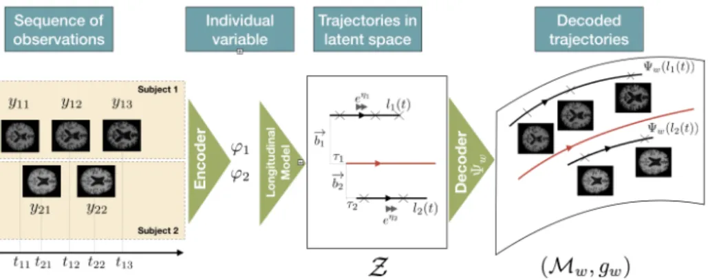
features from the images which are then fed to the RNN. In this case, both the convolutional network and the recurrent network are trained jointly by back-propagation. Figure 1 summarizes the whole procedure.
Fig. 1: The observed sequences are encoded into latent trajectories, which are then decoded into geodesics on a submanifold of the observation space.
2.4 Regularization
To impose some structure in the latent space Z, we impose a regularization on the individual variables ϕi = (ηi, τi, b2i, . . . , bdi). The regularization cost used is:
r(η, τ, b2, . . . , bd) = (η − η) 2 σ2 η +(τ − τ ) 2 σ2 τ + d X j=2 (bj)2 (2)
This regularization requires the individual variables η and τ to be close to mean values τ , η. The parameters η, τ are estimated during the inference. ση > 0 is
fixed but the estimation of η allows to adjust the typical variation of η with respect to the mean pace η, while the neural network Ψw adjusts accordingly
the actual velocity in the observation space in the e1 direction. στ is set to the
empirical standard deviation of the time distribution (tij)ij, meaning that we
expect the delays between subjects to be of the same order as the standard deviation of the visit ages.
2.5 Cost function and inference Overall, we optimize the cost function:
c(θ, w, η, τ ) =X i X j kyi(tij) − yijk22 σ2 + X i r(ϕi) (3)
where σ > 0 is a parameter controlling the trade-off reconstruction/regularity. The first term contains the requirements that the geometry (Mw, gw) be
adapted to the observed progressions since it requires geodesics yi(t) to be good
reconstructions of the individual trajectories. As shown in the Appendix, there exists solutions to problems of this kind: under mild conditions there exists a metric on a Riemannian manifold that the subjects progressions are geodesics. But this is only a partial constraint: there is a whole class of metrics which have geodesics in common (see [13] for the analysis of metrics which have a given family of trajectories as geodesics).
We infer the parameters of the model by stochastic gradient descent using the Adam optimizer [9]. After each batch of subjects B, we balance regularity and reconstruction by imposing a closed-form update on σ:
σ2= 1 NBD X i∈B Ni X j=1 kΨw(li(tij)) − yijk22 (4)
where NB =Pi∈BNi is the total number of observations in the batch b. This
automatic update of the trade-off criterion σ is inspired from Bayesian generative models which estimate the variance of the residual noise, as in e.g. [14, 20].
3
Experimental results
The neural network architectures and the source code for these experiments is available at gitlab.icm-institute.org/maxime.louis/unsupervised_geometric_ longitudinal, tag IPMI 2019. For all experiments, the ages of the subjects are first normalized to have zero mean and unit variance. This allows the positions in the latent space to remain close to 0. We set ση = 0.5 and initialize η to 0.
3.1 On a synthetic set of images
Fig. 2: Each row repre-sents a synthetic subject. To validate the proposed methodology, we first
per-form a set of experiments on a synthetic data set. We generate 64×64 gray level images of a white cross on a black background. Each cross is described by the arms length and angles. We prescribe a mean sce-nario of progression for the arm lengths and sample the arm angles for each subject from a zero-centered normal distribution. Figure 2 shows subjects gener-ated along this procedure. Note that with this set-ting, an image varies smoothly with respect to the arms lengths and angles and hence the whole set of generated images is a smooth manifold.
We generate 10 training sets of 150 subjects and
10 test sets of 50 subjects. The number of observation of each subject is randomly sampled from a Poisson distribution with mean 5. The times at which the subject
are observed are equally spaced within a randomly selected time window. We add different level of white noise on the images. We then run the inference on the 10 training sets for each level of noise. We set the dimension of the latent space Z to 3 for all the experiments.
For each run, we estimate the reconstruction error on both training set and test set, as well as the reconstruction error to the de-noised images, which were not seen during training. Results are shown on Figure 3.
0. 0.02 0.05 0.1
Standard deviation of added noise
0. 0.02 0.05 0.1
Mean squared error
Train Test Denoised train Denoised test
Fig. 3: Reconstruction error on train and test sets and on denoised train and test sets, unseen during training.
The model generalizes well to unseen data and successfully denoises the im-ages, with a reconstruction error on the denoised images which does not vary with the scale of the added white noise. This means that the generated manifold of images is close to the man-ifold on which the original images lie. Besides, as shown on Figure 4, the sce-nario of progression along the e1
di-rection is well captured, while orthog-onal directions e2, e3 allow to change
the arm positions. Finally, we com-pare the individual variables (b2
i, b3i)
to the known arms angles which were used to generate the images. Figure 5 shows the results: the latent space is structured in a way that is faithful to the original arm angles.
3.2 On cognitive scores
We use the cognitive scores grading the subjects memory, praxis, language and concentration from the ADNI database as in [14]. Each score is renormalized to vary between 0 and 1, with large values indicating poor performances for the task. Overall, the data set consists of 223 subjects observed 6 times on average over 2.9 years. We perform a 10-fold estimation of the model. The measured mean squared reconstruction error is 0.079 ± 1.1e − 3 on the train sets, while it is of 0.085 ± 1.5e − 3 for the test sets. Both are close to the uncertainty in the estimation of these cognitive scores [18]. This illustrates the ability of the model to generalize to unseen observations. First, this indicates that Mw is
a submanifold which is close to all the observations. Second, it indicates how relevant the learned Riemannian metric is, since unobserved subject trajectories are very close to geodesics on the Riemannian manifold.
Figure 6 shows obtained average trajectories t 7→ Ψw(eηe0(t − τ )) for a
10-fold estimation of the model on the data set, with Z dimension set to 2. All of these trajectories are brought back to a common time reference frame using the estimated τ and η. All average trajectories are very similar, underlining the stability of the proposed method. Note that despite the small average observation
Fig. 4: First row is t 7→ Ψθ(e1t). Following rows
are t 7→ Ψθ(e1t + ei) for i ∈ {2, 3}. These parallel
directions of progression show the same arm length reduction with different arm positions.
Fig. 5: Individual variables b1
i and b2i
colored by left (top) and right (bottom) arm angle.
time of the subjects, the method proposed here allows to robustly obtain a mean scenario of progression over 30 years. Hence, despite all the flexibility that is provided through the different neural networks and the individual parameters, the model still exhibits a low variance.
We compare the results to the mean trajectory estimated by the model [14], which is shown on Figure 8. Both cases recover the expected order of onset of the different cognitive symptoms in the disease progression. Note that with
60 65 70 75 80 Time 0.0 0.2 0.4 0.6 0.8 1.0
Normalized cognitive scores
memory language praxis concentration
Fig. 6: Learned main progression of the cog-nitive scores, for the 10-fold estimation. 60 65 70 75 80 Time 0.0 0.2 0.4 0.6 0.8 1.0
Normalized cognitive scores
memory language praxis concentration
Fig. 7: Mean geodesic of progression and par-allel variations t 7→ Ψ (eηe0(t − τ ) + λe1) for varying λ. 60 65 70 75 80 Time 0.0 0.1 0.2 0.3 0.4 0.5
Normalized cognitive scores
memory language praxis concentration
Fig. 8: Mean geodesic of progression and parallel variations for the model with user-defined met-ric.
our model the progression of the concentration score is much faster than the progression of the memory score, although it starts later: this type of behaviour is not allowed with the model described in [14] where the family of possible trajectories is much narrower. Indeed, because it is difficult to craft a relevant Riemannian metric for the data at hand, the authors modelled the data as lying on a product Riemannian manifold. In this case, a geodesic on the product manifold is a product of geodesics of each manifold. This strongly restricts the type of dynamics spanned by the model and hence gives it a high bias.
The use of the product manifold also has an impact on the parallel variations around the mean scenario: they can only delay and slow/accelerate one of the component with respect to another, as shown on Figure 8. Figure 7 illustrates the parallel variations Ψ (αe0(t − τ ) + e1) one can observe with the proposed model.
The variation is less trivial since complex interactions between each features are possible. In particular, the concentration score varies more in the early stages of the disease than in the late stages.
The individual variables ϕ. To show that the individual variables ϕi did
capture information regarding the disease progression, we compare the distribu-tion of the τibetween subjects who have at least one APOE4 allele of the APOE
gene -an allele known to be a implicated in Alzheimer’s disease- and subjects which have no APOE4 allele of this gene. We perform a Mann-Whitney test on the distributions to see if they differ. For all folds, a p-value lower than 5% is obtained. For all folds, carriers have a larger τ meaning that they have an earlier disease onset than non-carriers. This is in accordance with [2]. Similarly, women have on average an earlier disease onset for all folds, in accordance with [11].
Learned geometry
Memory
Concentration
Isomap
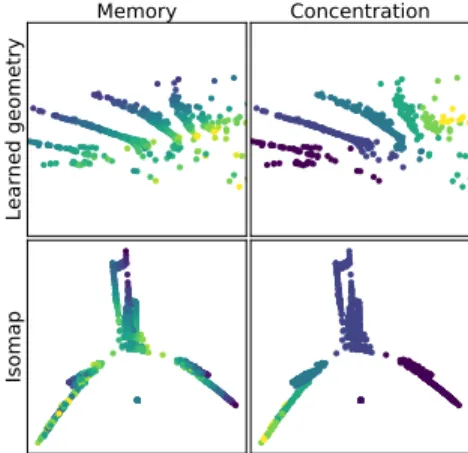
Fig. 9: Top (resp. Bottom) latent po-sitions (resp. Isomap embedding) of the observations colored by memory and concentration score.
A closer look at the geometry We look at the obtained Riemannian geome-try by computing the latent position best mapped onto each of the observation by Ψw. We then plot the obtained latent
po-sitions to look at the structure of the learned Riemannian manifold. We com-pare the obtained structure with a visual-isation of the structure induced by the `2 on the space of observations produced by Isomap [19]. Isomap is a manifold learning technique which attempts to reconstruct in low dimensions the geodesic distances computed from a set of observations. The results are shown on Figure 9. The ge-ometry obtained after inference is clearly much more suited for disease progression modelling. Indeed, the e1 direction does
dif-Fig. 10: t 7→ Ψθ(e0t) on the MRI dataset. The growth of the ventricles,
caracter-istic of aging and Alzheimer’s disease is clearly visible.
ferent scores. The induced metric is not as adapted. This highlights the relevance of the learned geometry for disease modelling.
3.3 On anatomical MRIs
We propose here an estimation of the model on 3D MRIs preprocessed from the ADNI database, to check the behaviour of the proposed method in high dimension. We select subjects which ultimately convert to Alzheimer’s disease. We obtain 325 subjects and a total of 1996 MRIs which we affinely align on the Colin-27 template and resample to 64x64x64. We run a 5-fold estimation of the model with dim Z = 10, using a GPU backend. We obtain a train mean squared error of 0.002 ± 1e − 5 and a test mean squared error of 0.0024 ± 3e − 5. Figure 10 shows one of the learned mean trajectory.
Once the model is estimated, we compare the distributions of the pace of progressions ηi between the individuals who have at least one APOE4 allele of
the APOE gene and the individuals who have no APOE4 allele. For all 5 folds, the distributions of the paces of progression significantly differ, with p-values lower than 5% and in each case, the APOE4 carriers have a greater pace of progression, in accordance with [2]. The same analysis between the individuals who have two APOE4 allele versus the individuals which have at maximum one APOE4 allele shows a significative difference for all folds for the τ variable: the APOE4 carriers have an earlier disease onset, as shown in [11]. This analysis further shows the value of the individual variables ϕi learned for each subject.
4
Conclusion
We presented a way to perform Riemannian geometry learning in the context of longitudinal trajectory analysis. We showed that we could build a local Rie-mannian submanifold of the space of observations which is so that each subject follows a geodesic parallel to a main geodesic of progression on this manifold. We illustrated how the encoding of each subject into these trajectories is infor-mative of the disease progression. The latent space Z built in this process is a
low-dimensional description of the disease progression. There are several possi-ble continuations of this work. First, there is the possibility to conduct the same analysis on multiple modalities of data simultaneously. Then, after estimation, the latent space Z could be useful to perform classification and prediction tasks. Acknowledgements This work has been partially funded by the European Re-search Council (ERC) under grant agreement No 678304, European Union’s Horizon 4582020 research and innovation programme under grant agreement No 666992, and the program ”Investissements d’avenir” ANR-10-IAIHU-06.
References
1. Arvanitidis, G., Hansen, L.K., Hauberg, S.: A locally adaptive normal distribution. In: Advances in Neural Information Processing Systems. pp. 4251–4259 (2016) 2. Bigio, E., Hynan, L., Sontag, E., Satumtira, S., White, C.: Synapse loss is greater in
presenile than senile onset alzheimer disease: implications for the cognitive reserve hypothesis. Neuropathology and applied neurobiology 28(3), 218–227 (2002)
3. Bˆone, A., Colliot, O., Durrleman, S.: Learning distributions of shape trajectories
from longitudinal datasets: a hierarchical model on a manifold of diffeomorphisms. arXiv preprint arXiv:1803.10119 (2018)
4. Cui, R., Liu, M., Li, G.: Longitudinal analysis for alzheimer’s disease diagnosis us-ing rnn. In: Biomedical Imagus-ing (ISBI 2018), 2018 IEEE 15th International Sym-posium on. pp. 1398–1401. IEEE (2018)
5. Gao, L., Pan, H., Liu, F., Xie, X., Zhang, Z., Han, J., Initiative, A.D.N., et al.: Brain disease diagnosis using deep learning features from longitudinal mr images. In: Asia-Pacific Web (APWeb) and Web-Age Information Management (WAIM) Joint International Conference on Web and Big Data. pp. 327–339. Springer (2018) 6. Hauberg, S., Freifeld, O., Black, M.J.: A geometric take on metric learning. In:
Advances in Neural Information Processing Systems. pp. 2024–2032 (2012) 7. Jack Jr, C.R., Bernstein, M.A., Fox, N.C., Thompson, P., Alexander, G., Harvey,
D., Borowski, B., Britson, P.J., L. Whitwell, J., Ward, C., et al.: The alzheimer’s disease neuroimaging initiative (adni): Mri methods. Journal of Magnetic Res-onance Imaging: An Official Journal of the International Society for Magnetic Resonance in Medicine 27(4), 685–691 (2008)
8. Jacobsen, J.H., Smeulders, A., Oyallon, E.: i-revnet: Deep invertible networks. arXiv preprint arXiv:1802.07088 (2018)
9. Kingma, D.P., Ba, J.: Adam: A method for stochastic optimization. arXiv preprint arXiv:1412.6980 (2014)
10. Koval, I., Schiratti, J.B., Routier, A., Bacci, M., Colliot, O., Allassonni`ere, S.,
Dur-rleman, S., Initiative, A.D.N., et al.: Statistical learning of spatiotemporal patterns from longitudinal manifold-valued networks. In: International Conference on Med-ical Image Computing and Computer-Assisted Intervention. pp. 451–459. Springer (2017)
11. Lam, B., Masellis, M., Freedman, M., Stuss, D.T., Black, S.E.: Clinical, imaging, and pathological heterogeneity of the alzheimer’s disease syndrome. Alzheimer’s research & therapy 5(1), 1 (2013)
12. Lebanon, G.: Learning riemannian metrics. In: Proceedings of the Nineteenth con-ference on Uncertainty in Artificial Intelligence. pp. 362–369. Morgan Kaufmann Publishers Inc. (2002)
13. Matveev, V.S.: Geodesically equivalent metrics in general relativity. Journal of Geometry and Physics 62(3), 675–691 (2012)
14. Schiratti, J.B., Allassonniere, S., Colliot, O., Durrleman, S.: Learning spatiotem-poral trajectories from manifold-valued longitudinal data. In: Advances in Neural Information Processing Systems. pp. 2404–2412 (2015)
15. Shao, H., Kumar, A., Fletcher, P.T.: The riemannian geometry of deep generative models. arXiv preprint arXiv:1711.08014 (2017)
16. Singh, N., Hinkle, J., Joshi, S., Fletcher, P.T.: Hierarchical geodesic models in diffeomorphisms. International Journal of Computer Vision 117(1), 70–92 (2016) 17. Sommer, S., Arnaudon, A., Kuhnel, L., Joshi, S.: Bridge simulation and metric
es-timation on landmark manifolds. In: Graphs in Biomedical Image Analysis, Com-putational Anatomy and Imaging Genetics, pp. 79–91. Springer (2017)
18. Standish, T.I., Molloy, D.W., B´edard, M., Layne, E.C., Murray, E.A., Strang,
D.: Improved reliability of the standardized alzheimer’s disease assessment scale (sadas) compared with the alzheimer’s disease assessment scale (adas). Journal of the American Geriatrics Society 44(6), 712–716 (1996)
19. Tenenbaum, J.B., De Silva, V., Langford, J.C.: A global geometric framework for nonlinear dimensionality reduction. science 290(5500), 2319–2323 (2000)
20. Zhang, M., Fletcher, T.: Probabilistic principal geodesic analysis. In: Advances in Neural Information Processing Systems. pp. 1178–1186 (2013)
A
Existence of a Riemannian metric such that a family
of curves are geodesics
Theorem 1. Let M be a smooth manifold and (γi)i∈{1,...,n} be a family of
smooth regular injective curves on M which do not intersect. There exists a Riemannian metric g such that γi is a geodesic on (M, g) for all i ∈ {1, . . . , n}.
Proof. Open neighborhood of the curves. Let i ∈ I. Since γi is injective and
regular, γi([0, 1]) is a submanifold of M. By the tubular neighborhood theorem,
there exists a vector bundle Ei on γi([0, 1]) and a diffeomorphism Φi from a
neighborhood Ui of the 0-section in Ei to a neighborhood Vi of γi([0, 1]) in M
such that Φi◦ 0Ei = ii where ii is the embedding of γi([0, 1]) in M. Without
loss of generality, we can suppose γj([0, 1]) ∩ Ui= ∅ for all j 6= i.
Riemannian metric on the neighborhoods. To do so, we use the fact that Ei
is diffeomorphic to the normal bundle on the segment [0, 1] ∈ R which is trivial and which we denote N . Let Ψi: Ei7→ N be such a diffeomorphism. Now N can
be equipped with a Riemannian metric hisuch that [0, 1] is a geodesic. Using Ψi
and Φi, we can push-forward the metric hi to get a metric gi on U which is so
that γi is a geodesic on (Ui, gi).
Stitching the metrics with a partition of unity. For each i ∈ {1, . . . , n}, pick an open subset Vi such that Vi ⊂ Vi ⊂ Ui and which contains γi([0, 1]), and set
O = M\(∪iVi). O is open so that C = {O, U1, . . . , Un} is an open cover of M. O
can be equipped with a metric gO(there always exists a Riemannian metric on a
smooth manifold). Finally, we use a partition of the unity ρO, ρ1, . . . , ρnon C and
set g = ρOgO+Piρigi. g is a Riemannian metric on M as a positive combination
In [13], the authors deal with a more general case but obtain a less explicit existence result. This theorem motivates our approach even if in equation (3) we ask for more: we want the existence a system of coordinates adapted to the progression.