HAL Id: hal-01104691
https://hal.archives-ouvertes.fr/hal-01104691
Preprint submitted on 19 Jan 2015
HAL is a multi-disciplinary open access
archive for the deposit and dissemination of
sci-entific research documents, whether they are
pub-lished or not. The documents may come from
teaching and research institutions in France or
abroad, or from public or private research centers.
L’archive ouverte pluridisciplinaire HAL, est
destinée au dépôt et à la diffusion de documents
scientifiques de niveau recherche, publiés ou non,
émanant des établissements d’enseignement et de
recherche français ou étrangers, des laboratoires
publics ou privés.
Asymmetric Parallel 3D Thinning Scheme and
Algorithms Based on Isthmuses
Michel Couprie, Gilles Bertrand
To cite this version:
Michel Couprie, Gilles Bertrand. Asymmetric Parallel 3D Thinning Scheme and Algorithms Based on
Isthmuses. 2015. �hal-01104691�
Asymmetric Parallel 3D Thinning Scheme and Algorithms Based on Isthmuses
MichelCouprie1,∗∗, GillesBertrand1aUniversit´e Paris-Est, LIGM, ´Equipe A3SI, ESIEE Paris, France
ABSTRACT
Critical kernels constitute a general framework settled in the context of abstract complexes for the study of parallel thinning in any dimension. We take advantage of the properties of this framework, to propose a generic thinning scheme for obtaining “thin” skeletons from objects made of voxels. From this scheme, we derive algorithms that produce curve or surface skeletons, based on the notion of 1D or 2D isthmus. We compare our new curve thinning algorithm with all the published algorithms of the same kind, based on quantitative criteria. Our experiments show that our algorithm largely outperforms the other ones with respect to noise sensitivity. Furthermore, we show how to slightly modify our algorithms to include a filtering parameter that controls effectively the pruning of skeletons, based on the notion of isthmus persistence.
1. Introduction
The usefulness of skeletons in many applications of pat-tern recognition, computer vision, shape understanding etc. is mostly due to their property of topology preservation, and preservation of meaningful geometrical features. Here, we are interested in the skeletonization of objects that are made of vox-els (unit cubes) in a regular 3D grid, i.e., in a binary 3D im-age. In this context, topology preservation is usually obtained through the iteration of thinning steps, provided that each step does not alter the topological characteristics. In sequential thin-ning algorithms, each step consists of detecting and choosing a so-called simple voxel, that may be characterized locally (see Kong and Rosenfeld (1989); Saha et al. (1994); Couprie and Bertrand (2009)), and removing it. Such a process usually in-volves many arbitrary choices, and the final result may depend, sometimes heavily, on any of these choices. This is why par-allel thinning algorithms are generally preferred to sequential ones. However, removing a set of simple voxels at each thin-ning step, in parallel, may alter topology. The framework of critical kernels, introduced by one of the authors in Bertrand (2007), provides a condition under which we have the guarantee that a subset of voxels can be removed without changing topol-ogy. This condition is, to our knowledge, the most general one
∗∗Corresponding author: Tel.: +33 1 45 92 66 88; fax: +33 1 45 92 66 99;
e-mail: [email protected] (Michel Couprie)
among the related works. Furthermore, critical kernels indeed provide a method to design new parallel thinning algorithms, in which the property of topology preservation is built-in, and in which any kind of constraint may be imposed (see Bertrand and Couprie (2008, 2014)).
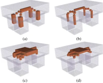
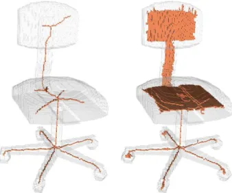
Among the different parallel thinning algorithms that have been proposed in the literature, we can distinguish between symmetric and asymmetric algorithms. Symmetric algorithms Ma (1995); Ma and Sonka (1996); Manzanera et al. (2002); Lo-hou and Bertrand (2007); Pal´agyi (2008) (also known as fully parallel algorithms) produce skeletons that are invariant under 90 degrees rotations. They consist of the iteration of thinning steps that are made of 1) the identification and selection of a set of voxels that satisfy certain conditions, independently of ori-entation or position in space, and 2) the removal, in parallel, of all selected voxels from the object. Symmetric algorithms, on the positive side, produce a result that is uniquely defined: no arbitrary choice is needed. On the negative side, they generally produce thick skeletons, see Fig. 1.
Asymmetric skeletons, on the opposite, are preferred when thinner skeletons are required. The price to pay is a certain amount of arbitrary choices to be made. In all existing asym-metric parallel thinning algorithms, each thinning step is di-vided into a certain number of substeps. In the so-called direc-tional algorithms Tsao and Fu (1981, 1982); Gong and Bertrand (1990); Pal´agyi and Kuba (1998); Pal´agyi and Kuba (1999a,b); Lohou and Bertrand (2004, 2005); Raynal and Couprie (2011); N´emeth et al. (2011), each substep is devoted to the detection
(a) (b)
(c) (d)
Fig. 1. Different types of skeletons. (a): Curve skeleton, symmetric. (b): Curve skeleton, asymmetric. (c): Surface skeleton, symmetric. (d): Sur-face skeleton, asymmetric.
and the deletion of voxels belonging to one “side” of the ob-ject: all the voxels considered during the substep have, for ex-ample, their south neighbor inside the object and their north neighbor outside the object. The order in which these direc-tional substeps are executed is set beforehand, arbitrarily. Sub-grid (or subfield) algorithms (see Bertrand and Aktouf (1995); Saha et al. (1997); Ma et al. (2002a,b); N´emeth et al. (2010a,b)) form the second category of asymmetric parallel thinning algo-rithms. There, each substep is devoted to the detection and the deletion of voxels that belong to a certain subgrid, for example, all voxels that have even coordinates. Considered subgrids must form a partition of the grid. Again, the order in which subgrids are considered is arbitrary.
Subgrid algorithms are not often used in practice because they produce artifacts, that is, waving skeleton branches where the original object is smooth or straight. Directional algorithms are the most popular ones. Most of them are implemented through sets of masks, one per substep. A set of masks is used to characterize voxels that must be kept during a given substep, in order to 1) preserve topology, and 2) prevent curves or sur-faces to disappear. Thus, topological conditions and geometri-cal conditions cannot be easily distinguished, and the slightest modification of any mask involves the need to make a new proof of the topological correctness.
Our approach is radically different. Instead of considering single voxels, we consider cliques. A clique is a set of mutually adjacent voxels. Then, we identify the critical kernel of the ob-ject, according to some definitions, which is a union of cliques. The main theorem of the critical kernels framework Bertrand (2007); Bertrand and Couprie (2014) states that we can remove in parallel any subset of the object, provided that we keep at least one voxel of every clique that constitutes the critical ker-nel, and this guarantees topology preservation. Here, as we try to obtain thin skeletons, our goal is to keep, whenever possible, exactly one voxel in every such clique. This leads us to propose
a generic parallel asymmetric thinning scheme, that may be en-riched by adding any sort of geometrical constraint. From our generic scheme, we easily derive, by adding such geometrical constraints, specific algorithms that produce curve or surface skeletons. To this aim, we define in this paper the notions of 1D and 2D isthmuses that capture relevant geometrical infor-mation: a 1D (resp. 2D) isthmus is a voxel that is “locally like a piece of curve” (resp. surface).
Our article is organized as follows. The first three sections contain a minimal set of basic notions about voxel complexes, simple voxels and critical kernels, respectively, which are nec-essary to make the article self-contained. In section 5, we intro-duce our new generic asymmetric thinning scheme, and we pro-vide some examples of ultimate skeletons obtained by using it. Section 6 is devoted to introducing and illustrating our new isthmus-based parallel algorithms for computing curve, surface and curve-surface skeletons. Then in section 7, we describe the experiments that we made for comparing our curve thinning al-gorithm with all existing parallel curve thinning methods of the same kind. We show that our method ranks first with respect to robustness. Finally, we show in section 8 how to use the notion of isthmus persistence in order to effectively filter the spurious skeleton parts due to noise. Persistence is a criterion, easy to compute in our framework, that allows us to dynamically de-tect or ignore certain isthmuses.
2. Voxel Complexes
In this section, we give some basic definitions for voxel complexes, see also Kovalevsky (1989); Kong and Rosenfeld (1989).
Let Z be the set of integers. We consider the families of sets F1 0, F 1 1, such that F 1 0 ={{a} | a ∈ Z}, F 1 1 ={{a, a + 1} | a ∈ Z}.
A subset f of Zn, n ≥ 2, that is the Cartesian product of exactly delements of F11and (n − d) elements of F10is called a face or an d-face of Zn, d is the dimension of f . In the illustrations of this paper, a 3-face (resp. 2-face, 1-face, 0-face) is depicted by a cube (resp. square, segment, dot), see e.g. Fig. 4.
A 3-face of Z3is also called a voxel. A finite set that is
com-posed solely of voxels is called a (voxel) complex (see Fig. 2). We denote by V3the collection of all voxel complexes.
We say that two voxels x, y are adjacent if x ∩ y , ∅. We write N(x) for the set of all voxels that are adjacent to a voxel x, N(x) is the neighborhood of x. Note that, for each voxel x, we have x ∈ N(x). We set N∗(x) = N(x) \ {x}.
Let d ∈ {0, 1, 2}. We say that two voxels x, y are d-neighbors if x∩y is a d-face. Thus, two distinct voxels x and y are adjacent if and only if they are d-neighbors for some d ∈ {0, 1, 2}.
Let X ∈ V3. We say that X is connected if, for any x, y ∈ X, there exists a sequence hx0, ...,xki of voxels in X such that x0=
x, xk= y, and xiis adjacent to xi−1, i = 1, ..., k.
3. Simple Voxels
Intuitively a voxel x of a complex X is called a simple voxel if its removal from X “does not change the topology of X”. This
b
a
c
d e
f
h
g
b
f
h
d
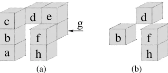
(a) (b)Fig. 2. (a) A complex X which is made of 8 voxels, (b) A complex Y ⊆ X, which is a thinning of X.
notion may be formalized with the help of the following re-cursive definition introduced in Bertrand and Couprie (2014), see also Kong (1997); Bertrand (1999) for other recursive ap-proaches for simplicity.
Definition 1. Let X ∈ V3.
We say that X is reducible if either: i) X is composed of a single voxel; or
ii) there exists x ∈ X such that N∗(x) ∩ X is reducible and X \ {x} is reducible.
Definition 2. Let X ∈ V3. A voxel x ∈ X is simple for X if
N∗(x) ∩ X is reducible. If x ∈ X is simple for X, we say that X \ {x}is an elementary thinning of X.
Thus, a complex X ∈ V3is reducible if and only if it is
possi-ble to reduce X to a single voxel by iteratively removing simple voxels. Observe that a reducible complex is necessarily non-empty and connected.
In Fig. 2 (a), the voxel a is simple for X (N∗(a) ∩ X is made
of a single voxel), the voxel d is not simple for X (N∗(d) ∩ X is
not connected), the voxel h is simple for X (N∗(h) ∩ X is made
of two voxels that are 2-neighbors and is reducible).
In Bertrand and Couprie (2014), it was shown that the above definition of a simple voxel is equivalent to classical characteri-zations based on connectivity properties of the voxel’s neigh-borhood Bertrand and Malandain (1994); Bertrand (1994); Saha et al. (1994); Kong (1995); Couprie and Bertrand (2009). An equivalence was also established with a definition based on the operation of collapse Whitehead (1939); Giblin (1981), this operation is a discrete analogue of a continuous deformation (a homotopy), see also Kong (1997); Bertrand (2007); Couprie and Bertrand (2009).
The notion of a simple voxel allows one to define thinnings of a complex, see an illustration Fig. 2 (b).
Let X, Y ∈ V3. We say that Y is a thinning of X or that X is reducible to Y, if there exists a sequence hX0, ...,Xki such that X0 = X, Xk = Y, and Xi is an elementary thinning of Xi−1,
i =1, ..., k.
Thus, a complex X is reducible if and only if it is reducible to a single voxel.
4. Critical Kernels
Let X be a complex in V3. It is well known that, if we
re-move simultaneously (in parallel) simple voxels from X, we may “change the topology” of the original object X. For exam-ple, the two voxels f and g are simple for the object X depicted
Fig. 2 (a). Nevertheless X\{ f , g} has two connected components whereas X is connected.
In this section, we recall a framework for thinning in paral-lel discrete objects with the warranty that we do not alter the topology of these objects Bertrand (2007); Bertrand and Cou-prie (2008, 2014). This method is valid for complexes of arbi-trary dimension.
Let d ∈ {0, 1, 2, 3} and let C ∈ V3. We say that C is a d-clique
or a clique if ∩{x ∈ C} is a d-face. If C is a d-clique, d is the rank of C.
If C is made of solely two distinct voxels x and y, we note that C is a d-clique if and only if x and y are d-neighbors, with d ∈ {0, 1, 2}.
Let X ∈ V3 and let C ⊆ X be a clique. We say that C is essential for Xif we have C = D whenever D is a clique such that:
i) C ⊆ D ⊆ X; and ii) ∩{x ∈ C} = ∩{x ∈ D}.
Observe that any complex C that is made of a single voxel is a clique (a 3-clique). Furthermore any voxel of a complex X constitutes a clique that is essential for X.
In Fig. 2 (a), { f , g} is a 2-clique that is essential for X, {b, d} is a 0-clique that is not essential for X, {b, c, d} is a 0-clique essential for X, {e, f , g} is a 1-clique essential for X.
Definition 3. Let S ∈ V3. The K -neighborhood of S , written
K (S ), is the set made of all voxels that are adjacent to each voxel in S . We set K∗(S ) = K (S ) \ S .
We note that we have K (S ) = N(x) whenever S is made of a single voxel x. We also observe that we have S ⊆ K (S ) whenever S is a clique.
Definition 4. Let X ∈ V3and let C be a clique that is essential
for X. We say that the clique C is regular for X if K∗(C) ∩ X
is reducible. We say that C is critical for X if C is not regular for X.
Thus, if C is a clique that is made of a single voxel x, then C is regular for X if and only if x is simple for X.
In Fig. 2 (a), the cliques C1 = {b, c, d}, C2 = { f , g}, and
C3 = { f , h} are essential for X. We have K∗(C1) ∩ X = ∅,
K∗(C
2) ∩ X = {e, h}, and K∗(C3) ∩ X = {g}. Thus, C1and C2
are critical for X, while C3is regular for X.
The following result is a consequence of a general theo-rem that holds for complexes of arbitrary dimensions Bertrand (2007); Bertrand and Couprie (2014).
Theorem 5. Let X ∈ V3and let Y ⊆ X.
The complex Y is a thinning of X if any clique that is critical for X contains at least one voxel of Y.
See an illustration in Fig. 2(a) and (b) where the complexes Xand Y satisfy the condition of theorem 5. For example, the voxel d is a non-simple voxel for X, thus {d} is a critical 3-clique for X, and d belongs to Y. Also, Y contains voxels in the critical cliques C1={b, c, d}, C2={ f , g}, and the other ones.
5. A generic 3D parallel and asymmetric thinning scheme Our goal is to define a subset Y of a voxel complex X that is guaranteed to include at least one voxel of each clique that is critical for X. By theorem 5, this subset Y will be a thinning of X.
Let us consider the complex X depicted Fig. 3 (a). There are precisely three cliques that are critical for X:
- the 0-clique C1={b, c} (we have K∗(C1) ∩ X = ∅);
- the 2-clique C2={a, b} (we have K∗(C2) ∩ X = ∅);
- the 3-clique C3={b} (the voxel b is not simple).
Suppose that, in order to build a complex Y that fulfills the condition of theorem 5, we select arbitrarily one voxel of each clique that is critical for X. Following such a strategy, we could select c for C1, a for C2, and b for C3. Thus, we would have
Y = X, no voxel would be removed from X. Now, we observe that the complex Y′ ={b} satisfies the condition of theorem 5.
This complex is obtained by considering first the 3-cliques be-fore selecting a voxel in the 2-, 1-, or 0 cliques.
The complex X of Fig. 3 (b) provides another example of such a situation. There are precisely three cliques that are criti-cal for X:
- the 1-clique C1={e, f , g, h} (we have K∗(C1) ∩ X = ∅);
- the 1-clique C2={e, d, g} (we have K∗(C2) ∩ X = ∅);
- the 2-clique C3={e, g} (K∗(C3) ∩ X is not connected).
If we select arbitrarily one voxel of each critical clique, we could obtain the complex Y = { f , d, g}. On the other hand, if we consider the 2-cliques before the 1-cliques, we obtain either Y′ ={e} or Y′′ = {g}. In both cases the result is better in the sense that we remove more voxels from X.
This discussion motivates the introduction of the fol-lowing 3D asymmetric and parallel thinning scheme AsymThinningScheme (see also Bertrand and Couprie (2008, 2009, 2014) for other thinning schemes and properties of critical kernels). The main features of this scheme are the following:
- Taking into account the observations made through the two previous examples, critical cliques are considered according to their decreasing ranks (step 4). Thus, each iteration is made of four sub-iterations (steps 4-8). Voxels that have been previously selected are stored in a set Y (step 8). At a given sub-iteration, we consider voxels only in critical cliques included in X \ Y (step 6).
- Select is a function from V3to V3, the set of all voxels. More
precisely, Select associates, to each set S of voxels, a unique voxel x of S . We refer to such a function as a selection function. This function allows us to select a voxel in a given critical clique (step 7). A possible choice is to take for Select(S ), the first pixel of S in the lexicographic order of the voxels coordinates.
- In order to compute curve or surface skeletons, we have to keep other voxels than the ones that are necessary for the preservation of the topology of the object X. In the scheme, the set K corresponds to a set of features that we want to be preserved by a thinning algorithm (thus, we have K ⊆ X). This set K, called constraint set, is updated dynamically at step 10. SkelX is a function from X on {True, False} that allows us to
keep some skeletal voxels of X, e.g., some voxels belonging to
c
b
a
e
g
f
h
d
(a) (b)Fig. 3. Two complexes.
parts of X that are surfaces or curves. For example, if we want to obtain curve skeletons, a frequently employed solution is to set SkelX(x) = True whenever x is a so-called end voxel of X:
an end voxel is a voxel that has exactly one neighbor inside X. Better propositions for such a function will be introduced in section 6.
By construction, at each iteration, the complex Y at step 9 satisfies the condition of theorem 5. Thus, the result of the scheme is a thinning of the original complex X. Observe also that, except step 4, each step of the scheme may be computed in parallel.
Algorithm 1: AsymThinningScheme(X, SkelX)
Data: X ∈ V3, Skel
X is a function from X on {True, False}
Result: X K:= ∅; 1 repeat 2 Y:= K; 3 for d ← 3 to 0 do 4 Z:= ∅; 5
foreach d-clique C ⊆ X \ Y that is critical for X do
6 Z:= Z ∪ {Select(C)}; 7 Y:= Y ∪ Z; 8 X:= Y; 9
foreach voxel x ∈ X \ K such that SkelX(x) = True do
10
K:= K ∪ {x};
11
until stability ;
12
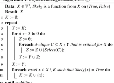
Fig. 4 provides an illustration of the scheme AsymThinningScheme. Let us consider the complex X depicted in (a). We suppose in this example that we do not keep any skeletal voxel, i.e., for any x ∈ X, we set SkelX(x) = False.
The traces of the cliques that are critical for X are represented in (b), the trace of a clique C is the face f = ∩{x ∈ C}. Thus, the set of the cliques that are critical for X is precisely composed of six 0-cliques, two 1-cliques, three 2-cliques, and one 3-clique. In (c) the four different sub-iterations of the first iteration of the scheme are illustrated (steps 4-8):
- when d = 3, only one clique is considered, the dark grey voxel is selected whatever the selection function;
- when d = 2, all the three 2-cliques are considered since none of these cliques contains the above voxel. Voxels that could be selected by a selection function are depicted in medium grey; - when d = 1, only one clique is considered, a voxel that could be selected is depicted in light grey;
(a) (b)
(c) (d)
(e) (f)
(g) (h)
Fig. 4. (a): A complex X made of precisely 12 voxels. (b): The traces of the cliques that are critical for X. (c): Voxels that have been selected by the algorithm. (d): The result Y of the first iteration. (e): The traces of the 4 cliques that are critical for Y. (f): The result of the second iteration. (g) and (h): Two other possible selections at the first iteration.
0-cliques contains at least one voxel that has been previously selected.
After these sub-iterations, we obtain the complex depicted in (d). The figures (e) and (f) illustrate the second iteration, at the end of this iteration the complex is reduced to a single voxel. In (g) and (h) two other possible selections at the first iteration are given.
Of course, the result of the scheme may depend on the choice of the selection function. This is the price to be paid if we try to obtain thin skeletons. For example, some arbitrary choices have to be made for reducing a two voxels wide ribbon to a simple curve.
Fig. 5 shows another illustration, on bigger objects, of AsymThinningScheme. Here also, for any x ∈ X, we have SkelX(x) = False (no skeletal voxel). The result is called an
ultimate asymmetric skeleton.
6. Isthmus-based asymmetric thinning
In this section, we show how to use our generic scheme AsymThinningScheme in order to get a procedure that com-putes either curve or surface skeletons. This thinning procedure preserves a constraint set K that is made of “isthmuses”.
Intuitively, a voxel x of an object X is said to be a 1-isthmus (resp. a 2-isthmus) if the neighborhood of x corresponds - up to
Fig. 5. Ultimate asymmetric skeletons obtained by using AsymThinningScheme. On the left, the object is a solid cylinder bent to form a knot. Its ultimate skeleton is a discrete curve. On the right, the object is connected and without holes and cavities. Its ultimate skeleton is a single voxel.
a thinning - to the one of a point belonging to a curve (resp. a surface) Bertrand and Couprie (2014).
We say that X ∈ V3is a 0-surface if X is precisely made of two voxels x and y such that x ∩ y = ∅.
We say that X ∈ V3is a 1-surface (or a simple closed curve) if:
i) X is connected; and ii) For each x ∈ X, N∗(x) ∩ X is a 0-surface.
Definition 6. Let X ∈ V3, let x ∈ X.
We say that x is a 1-isthmus for X if N∗(x) ∩ X is reducible to a 0-surface.
We say that x is a 2-isthmus for X if N∗(x) ∩ X is reducible to a 1-surface.
We say that x is a 2+-isthmus for X if x is a 1-isthmus or a 2-isthmus for X.
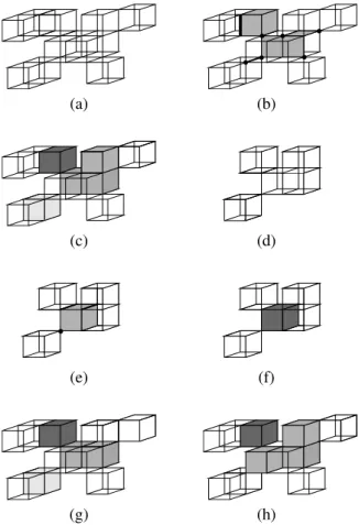
See Fig. 6 for an illustration of the notion of k-isthmus. Our aim is to thin an object, while preserving a constraint set Kthat is made of voxels that are detected as k-isthmuses during the thinning process. We obtain curve skeletons with k = 1, surface skeletons with k = 2, and surface/curve skeletons with k = 2+. These three kinds of skeletons may be obtained by usingAsymThinningScheme, with the function SkelX defined
as follows: SkelX(x) =
(
True if x is a k-isthmus for X, False otherwise,
with k being set to 1, 2, or 2+.
Observe that there is the possibility that a voxel belongs to a k-isthmus at a given step of the algorithm, but not at further steps. This is why previously detected isthmuses are stored (see lines 10-11 ofAsymThinningScheme).
In Fig. 7, we show a curvilinear skeleton and a sur-face/curvilinear skeleton obtained by our method from the same object.
x y
Fig. 6. First row: a voxel complex X. Second row: left, the set N∗(x)∩ X and
right, a 0-surface that is a thinning of N∗(x) ∩ X. Hence, x is a 1-isthmus.
Third row: left, the set N∗(y) ∩ X and right, a 1-surface that is a thinning
of N∗(y) ∩ X. Hence, x is a 2-isthmus.
7. Experiments, results and discussion
In these experiments, we used a database of 30 three-dimensional voxel objects. These objects were obtained by converting into voxel sets some 3D models freely available on the internet (mainly from the NTU 3D database, see http: //3d.csie.ntu.edu.tw/~dynamic/benchmark). Our test set can be downloaded at http://www.esiee.fr/~info/ ck/3DSkAsymTestSet.tgz. We chose these objects because they all may be well described by a curve skeleton, the branches of which can be intuitively related to object parts (for example, the skeleton of a coarse human body has typically 5 branches, one for the head and one for each limb). For each object, we manually indicated an “ideal” number of branches. Unneces-sary branches are essentially due to noise. Thus, a simple and effective criterion for assessing the robustness of a skeletoniza-tion method is to count the number of extra branches, or equiv-alently in our case, the number of extra curve extremities.
In order to compare methods, we mainly use the indicator E(X, M) = |c(X, M) − ci(X)|, where c(X, M) stands for the
num-ber of curve extremities for the result obtained from X after application of method M, and ci(X) stands for the ideal
num-ber of curve extremities to expect with the object X. Note that, for all objects in our database and all tested methods, the differ-ence was positive, in other words the methods produced more skeleton branches than expected, or just the right number. We define E(M) as the average, for all objects of the database, of E(X, M). The lower the value of E(M), the better the method M with respect to robustness.
Another useful indicator is the reconstruction ratio, defined as R(X, M) = 100×V(Re(SkV(X)(X,M),X)), where Sk(X, M) is the skele-ton obtained from object X using method M, Re(S , X) stands for the reconstruction from S (union of balls using the voxels of S as centers and the values of the distance map of X as radii), and
Fig. 7. Asymmetric skeletons obtained by using AsymThinningScheme. Left: curve skeleton. The function SkelXis based on 1-isthmuses. Right:
curve and surface skeleton. The function SkelX is based on 2+-isthmuses.
Of course, these skeletons need some filtering, see section 8 and Fig. 11.
V(X) stands for the number of voxels of X. We define R(M) as the average, for all objects of the database, of R(X, M). Of course, there is a trade-off between indicators R and E, as a noisy skeleton with many spurious branches will likely yield a high reconstruction rate. But for skeletons with comparable val-ues of E, a higher R indicates a better quality (better centering and/or longer skeleton branches).
The goal of asymmetric thinning is to provide “thin” skele-tons. This means in particular that the resulting skeletons should contain no simple voxel, apart from the curve extrem-ities. However, due to their parallel nature, most thinning al-gorithms considered in this study may leave some extra sim-ple voxels. We define our third indicator as P(X, M) = 100 ×
V(Si(Sk(X,M)))
V(Sk(X,M)) , where Si(S ) denotes the set of simple voxels of S
that are not curve extremities. We define P(M) as the average, for all objects of the database, of P(X, M). The lower the value of P(M), the better the method M with respect to thinness.
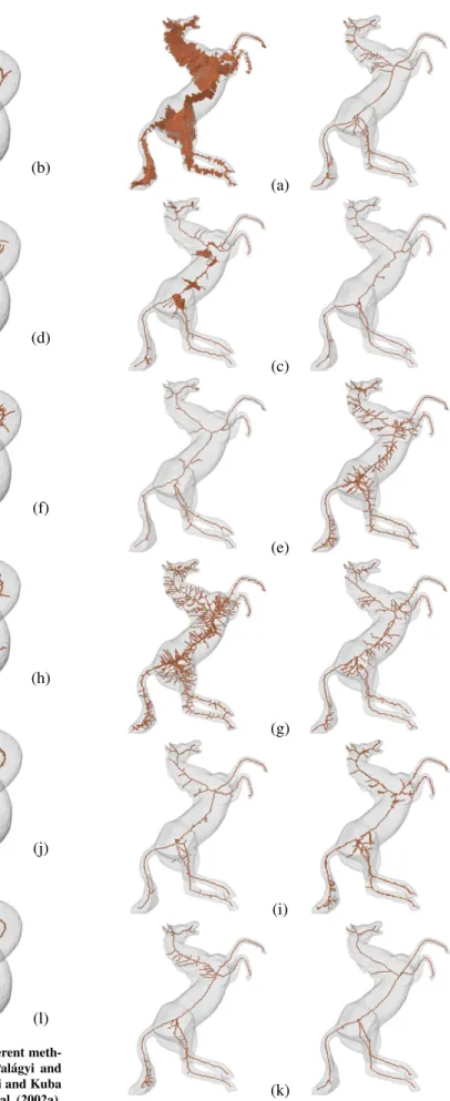
To make a fair comparison, we consider only parallel asym-metric thinning methods that produce curve skeletons of voxel objects, and that have no parameter. In particular, we do not consider the variants of the algorithms of N´emeth et al. (2010b) that involve the checking of extremity voxel neighborhoods of increasing size, as this neighborhood size is indeed a parameter. First of all, it is interesting to look at the results of different methods for a same object (see Fig. 8 and Fig. 9). We notice in particular that some methods, like Tsao and Fu (1981) and Pal´agyi and Kuba (1998), are not sufficiently powerful to pro-duce results that may be interpreted as curve skeletons (see also the ratio of remaining simple points in table 1). For the sake of space and readability, we selected only 12 methods among the 21 that took place in our experiments. See table 1 for the complete quantitative results.
(a) (b) (c) (d) (e) (f) (g) (h) (i) (j) (k) (l)
Fig. 8. Curve skeletons of a same object obtained through different meth-ods: (a) Tsao and Fu (1981), (b) Tsao and Fu (1982), (c) Pal´agyi and Kuba (1998), hybrid, (d) Pal´agyi and Kuba (1999a), (e) Pal´agyi and Kuba (1999b), (f) Ma and Wan (2000), (g) Ma et al. (2002b), (h) Ma et al. (2002a), (i) Lohou and Bertrand (2005), (j) N´emeth et al. (2010a), 2 subgrids, (k) N´emeth et al. (2010b), 8 subgrids, (l) Our new method based on isthmuses.
(a) (b) (c) (d) (e) (f) (g) (h) (i) (j) (k) (l)
Table 1. Results of our quantitative comparison (see text). The term “dir” indicates a directional algorithm, “sgr” a subgrid algorithm, and “hy-brid” an algorithm that alternates directional steps and subgrid steps. Our method AsymThinningScheme was used, either with a function SkelXthat
detects 1-isthmuses (1), or with a function that detects extremity voxels (2).
Method M E(M) R(M) P(M)
Tsao and Fu (1981), 6 dir 177.2 89.9 29.07
Tsao and Fu (1982), 6 dir 37.0 75.1 5.66
Gong and Bertrand (1990), 6 dir 134.1 92.5 28.15 Bertrand and Aktouf (1995), 8 sgr 15.6 72.6 0.13
Saha et al. (1997), 8 sgr 117.4 80.1 0.29
Pal´agyi and Kuba (1998), 6 dir 43.2 78.7 1.96 Pal´agyi and Kuba (1998), hybrid 25.7 78.0 8.28 Pal´agyi and Kuba (1999a), 8 dir 8.97 60.8 0.23 Pal´agyi and Kuba (1999b), 12 dir 9.2 51.3 0.72
Ma and Wan (2000), 6 dir 115.9 82.9 10.40
Ma et al. (2002b), 4 sgr 380.1 88.0 0.18
Ma et al. (2002a), 2 sgr 51.5 79.7 0.43
Lohou and Bertrand (2004), 12 dir 21.0 55.8 0.13 Lohou and Bertrand (2005), 6 dir 11.3 71.5 0.003 N´emeth et al. (2010a), 2 sgr 67.9 81.3 38.32
N´emeth et al. (2010b), 4 sgr 38.2 75.6 0.0
N´emeth et al. (2010b), 8 sgr 31.7 74.7 0.0
N´emeth et al. (2011), 6 dir 10.1 71.5 5.59
Raynal and Couprie (2011), 6 dir 12.9 74.3 1.56
AsymThinningScheme(1) 5.5 68.5 0.05
AsymThinningScheme(2) 6.7 68.8 0.0
This illustrates the difficulty of designing a method that keeps enough voxels in order to preserve topology, and in the same time, deletes a sufficient number of voxels in order to produce thin curve skeletons. This difficulty is indeed high when these two opposite constraints are not clearly distinguished. The strength of our approach lies in a complete separation of these constraints.
The example of Fig. 8 illustrates very well the sensitivity to contour noise of the methods. The original object is a solid cylinder bent in order to form a knot. Thus, its curve skeleton should ideally be a simple closed curve. Any extra branch of the skeleton must undoubtedly be considered as spurious. As can be seen in the figure, only our method produces a skeleton of this object that is totally free of spurious branches.
Table 1 gathers the quantitative results of our experiments, that allows us to compare the 19 other existing methods of the same class with our algorithm. We see that our method out-performs all existing methods with respect to the robustness criterion. This remains true if we use extremity voxels (vari-ant 2) instead of 1-isthmuses (vari(vari-ant 1) as skeletal voxels. We note also that, compared with the two best methods after ours, namely Pal´agyi and Kuba’s directional methods with 8 and 12 substeps, our algorithms have a better reconstruction ratio R(M) and thinness factor P(M).
8. Isthmus persistence and skeleton filtering
It is well known that the skeletonization process is highly sensitive to noise, and this is a major issue in practical appli-cations. The origin of this problem lies in the following fact: the transformation that associates its skeleton to a shape is not continuous. In practice, it means that if a small perturbation is applied on the contour of an object, then a big skeleton part may appear or disappear. See for example Attali et al. (2009) for a survey of selected studies on the stability of skeletons.
In consequence, many authors have proposed methods that aim at eliminating, or “pruning”, spurious skeleton branches or parts. These methods are essentially based on a criterion that permits to distinguish between points or parts of the skeleton, those that are due to noise from those that are robust to small perturbations.
Among the different criteria that were proposed in the liter-ature, the notion of isthmus persistence introduced in Liu et al. (2010) (see also Chaussard (2010)) yields a simple yet efficient method to filter skeletons during the thinning process. Origi-nally, this method has been formulated in the framework of 3D cubical complexes, i.e., objects made of faces of different di-mensions. In this section, we show that it can be adapted to the context of voxel complexes.
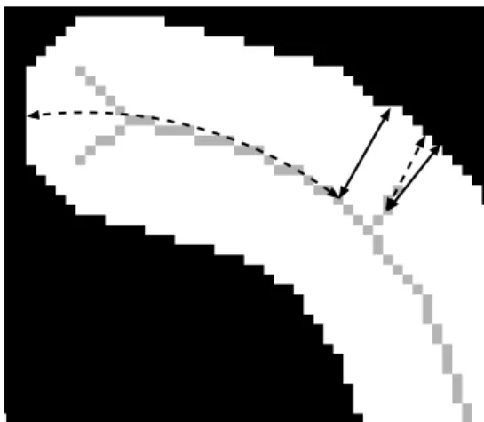
Let x be a voxel in a voxel complex X, that becomes an isth-mus for the first time at step i of the parallel thinning. Then, we define the birth date of x, denoted by b(x), as b(x) = i. In-tuitively, b(x) corresponds to the local thickness of the object around the voxel x, see Fig. 10 for an illustration in 2D.
Now, consider an isthmus voxel x that becomes, at step j of the parallel thinning process, a deletable voxel. Then, we define the death date of x, denoted by d(x), as d(x) = j.
Finally, we define the persistence of the voxel x as the dif-ference between the death date ane the birth date, that is, d(x) − b(x). It may be seen that a voxel with a high persistence value is likely to belong to a robust skeleton part, whereas a low persistence characterizes a voxel in a spurious skeleton part (Fig. 10). Therefore, skeleton filtering may be performed by keeping in the constraint set of the thinning algorithm, only the isthmuses that have a persistence greater than a given threshold.
Fig. 10. The lengths depicted with a solid line correspond to the birth dates, the dotted lines to the death dates.
In the following algorithm, k stands for the dimension of the considered isthmuses (1, 2 or 2+), and p is a parameter that
sets the persistence threshold. The function b associates to cer-tain voxels their birth date, and K is a constraint set that is dy-namically updated by adding those voxels whose persistence is greater than the threshold p (lines 12-13).
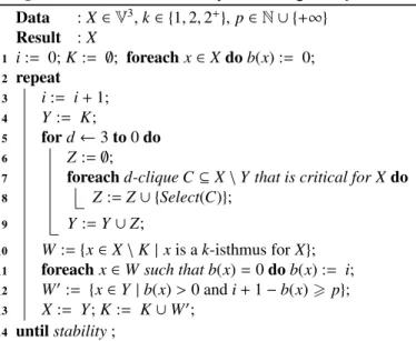
Algorithm 2: PersistenceAsymThinning(X, k, p) Data : X ∈ V3, k ∈ {1, 2, 2+}, p ∈ N ∪ {+∞} Result : X i:= 0; K := ∅; foreach x ∈ X do b(x) := 0; 1 repeat 2 i:= i + 1; 3 Y:= K; 4 for d ← 3 to 0 do 5 Z:= ∅; 6
foreach d-clique C ⊆ X \ Y that is critical for X do
7 Z:= Z ∪ {Select(C)}; 8 Y:= Y ∪ Z; 9 W:= {x ∈ X \ K | x is a k-isthmus for X}; 10
foreach x ∈ W such that b(x) = 0 do b(x) := i;
11 W′:= {x ∈ Y | b(x) > 0 and i + 1 − b(x) > p}; 12 X:= Y; K := K ∪ W′; 13 until stability ; 14
In line 11, the birth date b(x) of each new isthmus voxel x is recorded. In line 12, the test b(x) > 0 implies that the con-sidered voxel x has been recorded as an isthmus voxel. Fur-thermore, since this voxel x belongs to Y, it is not deletable, thus its death date d(x) is strictly greater than i. The condition i +1 − b(x) > p thus implies d(x) − b(x) > p, meaning that the voxel x must be added to the constraint set K (see line 13) because its persistence is greater than p.
Extreme cases for the values of the parameter p are p = 1 and p = +∞. Notice that, by the very definitions of isthmus and persistence, the persistence of any isthmus is at least one (since an isthmus is not deletable). If p = 1, then all detected isthmuses are added to the constraint set. In this case, we re-trieve the behaviour of algorithmIsthmusAsymThinnning. If p = +∞, then no voxel is added to the constraint set. In this case, the result is an ultimate asymmetric skeleton of X.
Fig. 12 illustrates the usefulness and the effectiveness of persistence-based filtering. Fig. 12(a) shows a 3D shape and its skeleton obtained by using AsymThinningScheme. In Fig. 12(b), we added some random noise to the shape contour. We clearly see that, for noisy objects, some filtering is manda-tory. We obtain satisfactory results with values of p greater than 5. See also Fig. 11.
9. Conclusion
We introduced an original generic scheme for asymmetric parallel topology-preserving thinning of 3D objects made of voxels, in the framework of critical kernels. We saw that from this scheme, one can easily derive several thinning operators having specific behaviours, simply by changing the definition
Fig. 11. Filtered skeletons of the same object as in Fig. 7. Left: curve skele-ton, p = 3. Right: curve and surface skeleskele-ton, p = 2.
of skeletal points. In particular, we showed that ultimate, curve, surface, and surface/curve skeletons can be obtained, based on the notion of 1D/2D isthmuses.
A key point, in the implementation of the algorithms pro-posed in this paper, is the detection of critical cliques and isth-mus voxels. In Bertrand and Couprie (2014), we showed that it is possible to detect critical cliques thanks to a set of masks, in linear time. Note also that the configurations of 1D and 2D isthmuses may be pre-computed by a linear-time algorithm and stored in lookup tables. Finally, based on a breadth-first strat-egy, the whole method can be implemented to run in O(n) time, where n is the number of voxels of the input 3D image.
We performed some experiments in order to compare our curve skeletonization algorithm with all methods of the same class found in the literature. The results show clearly that our method outperforms the other ones with respect to robustness.
Furthermore, we showed that an effective filtering can be eas-ily performed within our framework, thanks to the notion of persistence. In this approach, the filtering is done dynamically, with very little added cost, and is governed by a unique pa-rameter. Persistence is closely linked to the notion of isthmus, and we stress that this kind of filtering cannot be adapted to the other methods considered in our experiments.
Acknowledgments
This work has been partially supported by the “ANR-2010-BLAN-0205 KIDICO” project.
References
Attali, D., Boissonnat, J., Edelsbrunner, H., 2009. Stability and computation of the medial axis — a state-of-the-art report, in: M¨oller, T., Hamann, B., Rus-sell, B. (Eds.), Mathematical Foundations of Scientific Visualization, Com-puter Graphics, and Massive Data Exploration. Springer-Verlag, pp. 109– 125.
Bertrand, G., 1994. Simple points, topological numbers and geodesic neigh-borhoods in cubic grids. Pattern Recognition Letters 15, 1003–1011.
(a) (b)
(c) (d) (e)
Fig. 12. (a) Original shape and its curve skeleton obtained by us-ing AsymThinnus-ingScheme. (b) Noisy shape and its curve skele-ton. (c,d,e) Filtered skeletons of the noisy shape, obtained by using PersistenceAsymThinning, with parameter values 2, 5, 8 respectively.
Bertrand, G., 1999. New notions for discrete topology, in: Discrete Geometry for Computer Imagery, Springer. pp. 218–228.
Bertrand, G., 2007. On critical kernels. Comptes Rendus de l’Acad´emie des Sciences, S´erie Math. I, 363–367.
Bertrand, G., Aktouf, Z., 1995. Three-dimensional thinning algorithm using subfields, in: Vision Geometry III, SPIE. pp. 113–124.
Bertrand, G., Couprie, M., 2008. Two-dimensional thinning algorithms based on critical kernels. Journal of Mathematical Imaging and Vision 31, 35–56. Bertrand, G., Couprie, M., 2009. On parallel thinning algorithms: Minimal non-simple sets, P-simple points and critical kernels. Journal of Mathemat-ical Imaging and Vision 35, 23–35.
Bertrand, G., Couprie, M., 2014. Powerful Parallel and Symmetric 3D Thinning Schemes Based on Critical Kernels. Journal of Mathematical Imaging and Vision 48, 134–148.
Bertrand, G., Malandain, G., 1994. A new characterization of three-dimensional simple points. Pattern Recognition Letters 15, 169–175. Chaussard, J., 2010. Topological tools for discrete shape analysis. Ph.D.
dis-sertation. Universit´e Paris-Est.
Couprie, M., Bertrand, G., 2009. New characterizations of simple points in 2D, 3D and 4D discrete spaces. IEEE Transactions on Pattern Analysis and Machine Intelligence 31, 637–648.
Giblin, P., 1981. Graphs, surfaces and homology. Chapman and Hall. Gong, W., Bertrand, G., 1990. A simple parallel 3d thinning algorithm, in:
ICPR90, pp. 188–190.
Kong, T.Y., 1995. On topology preservation in 2-D and 3-D thinning.
Interna-tional Journal on Pattern Recognition and Artificial Intelligence 9, 813–844. Kong, T.Y., 1997. Topology-preserving deletion of 1’s from 2-, 3- and 4-dimensional binary images, in: Discrete Geometry for Computer Imagery, Springer. pp. 3–18.
Kong, T.Y., Rosenfeld, A., 1989. Digital topology: introduction and survey. Comp. Vision, Graphics and Image Proc. 48, 357–393.
Kovalevsky, V., 1989. Finite topology as applied to image analysis. Computer Vision, Graphics and Image Processing 46, 141–161.
Liu, L., Chambers, E.W., Letscher, D., Ju, T., 2010. A simple and robust thin-ning algorithm on cell complexes. Computer Graphics Forum 29, 2253– 2260.
Lohou, C., Bertrand, G., 2004. A 3D 12-subiteration thinning algorithm based on P-simple points. Discrete Applied Mathematics 139, 171–195. Lohou, C., Bertrand, G., 2005. A 3D 6-subiteration curve thinning algorithm
based on P-simple points. Discrete Applied Mathematics 151, 198–228. Lohou, C., Bertrand, G., 2007. Two symmetrical thinning algorithms for 3D
binary images. Pattern Recognition 40, 2301–2314.
Ma, C., Wan, S., Chang, H., 2002a. Extracting medial curves on 3D images. Pattern Recognition Letters 23, 895–904.
Ma, C.M., 1995. A 3D fully parallel thinning algorithm for generating medial faces. Pattern Recognition Letters 16, 83–87.
Ma, C.M., Sonka, M., 1996. A 3D fully parallel thinning algorithm and its applications. Computer Vision and Image Understanding 64, 420–433. Ma, C.M., Wan, S.Y., 2000. Parallel thinning algorithms on 3D (18,6) binary
images. Computer Vision and Image Understanding 80, 364–378. Ma, C.M., Wan, S.Y., Lee, J.D., 2002b. Three-dimensional topology preserving
reduction on the 4-subfields. IEEE Transactions on Pattern Analysis and Machine Intelligence 24, 1594–1605.
Manzanera, A., Bernard, T., Prˆeteux, F., Longuet, B., 2002. n-dimensional skeletonization: a unified mathematical framework. Journal of Electronic Imaging 11, 25–37.
N´emeth, G., Kardos, P., Pal´agyi, K., 2010a. Topology preserving 2-subfield 3D thinning algorithms, in: Signal Processing, Pattern Recognition and Appli-cations (SPPRA 2010). ACTA Press. volume 678, pp. 311–316.
N´emeth, G., Kardos, P., Pal´agyi, K., 2010b. Topology preserving 3D thin-ning algorithms using four and eight subfields, in: Campilho, A., Kamel, M. (Eds.), Image Analysis and Recognition. Springer Berlin / Heidelberg. volume 6111 of Lecture Notes in Computer Science, pp. 316–325. N´emeth, G., Kardos, P., Pal´agyi, K., 2011. A family of topology-preserving
3D parallel 6-subiteration thinning algorithms, in: Proc. 14th International Workshop on Combinatorial Image Analysis, IWCIA2011, Springer. pp. 17–30.
Pal´agyi, K., 2008. A 3D fully parallel surface-thinning algorithm. Theoretical Computer Science 406, 119–135.
Pal´agyi, K., Kuba, A., 1998. A 3D 6-subiteration thinning algorithm for ex-tracting medial lines. Pattern Recognition Letters , 613–627.
Pal´agyi, K., Kuba, A., 1998. A hybrid thinning algorithm for 3d medical im-ages. Journal of Computing and Information Technology 6, 149–164. Pal´agyi, K., Kuba, A., 1999a. Directional 3D thinning using 8 subiterations, in:
Discrete Geometry for Computer Imagery, Springer. pp. 325–336. Pal´agyi, K., Kuba, A., 1999b. A parallel 3D 12-subiteration thinning algorithm.
Graphical Models and Image Processing 61, 199–221.
Raynal, B., Couprie, M., 2011. Isthmus-based 6-directional parallel thinning al-gorithms, in: Discrete Geometry for Computer Imagery, Springer. pp. 141– 152.
Saha, P., Chaudhuri, B., Chanda, B., Dutta Majumder, D., 1994. Topology preservation in 3D digital space. Pattern Recognition 27, 295–300. Saha, P., Chaudhuri, B., Dutta Majumder, D., 1997. A new shape preserving
parallel thinning algorithm for 3d digital images. Pattern Recognition 30, 1939–1955.
Tsao, Y., Fu, K., 1981. A parallel thinning algorithm for 3D pictures. Computer Graphics and Image Processing 17, 315–331.
Tsao, Y., Fu, K., 1982. A 3D parallel skeletonwise thinning algorithm pictures, in: Pattern Recognition and Image Processing, pp. 678–683.
Whitehead, J., 1939. Simplicial spaces, nuclei and m-groups. Proceedings of the London Mathematical Society 45, 243–327.