Causal inference with time-series cross-sectional data : with applications to positive political economy

Causal Inference with Time-Series Cross-Sectional Data:

with Applications to Positive Political Economy

by

Yiqing Xu MASSACHUSETTS INSTI

M.A. in Economics

Peking University, 2010

JUN 13

20

LIBRARIES

ARCHNES

IN PARTIAL FULFILLMENT OF THE REQUIREMENTS FOR THE DEGREE OF DOCTOR OF PHILOSOPHY

AT THE

MASSACHUSETTS INSTITUTE OF TECHNOLOGY

TUTE

I

JUNE 2016

@

Signature of Author ...

Signature redacted

Department of Political Science April 14, 2016

Certified by ...

Accepted by ...

S ignature redacted...

Signature redacted

Ben Ross Schneider Ford International Professor of Political Science Chair, Graduate Program Committee

MITLibraries

77 Massachusetts Avenue

Cambridge, MA 02139 http://Iibraries.mit.edu/ask

DISCLAIMER NOTICE

Due to the condition of the original material, there are unavoidable flaws in this reproduction. We have made every effort possible to provide you with the best copy available.

Thank you.

The images contained in this document are of the ,best quality available.

Causal Inference with Time-Series Cross-Sectional Data:

with Applications to Positive Political Economy

by Yiqing Xu

Submitted to the Department of Political Science on April 14, 2016 in Partial Fulfillment of the Requirements

for the Degree of Doctor of Philosophy in Political Science

ABSTRACT

Time-series cross-sectional (TSCS) data are widely used in today's social sciences. Researchers often rely on two-way fixed effect models to estimate causal quantities of interest with TSCS data. However, they face the challenge that such models are not applicable when the so called "parallel trends" assumption fails, that is, the average treated counterfactual and average control outcome do not follow parallel paths.

The first chapter of this dissertation introduces the generalized synthetic control method that addresses this challenge. It imputes counterfactuals for each treated unit using control group information based on a linear interactive fixed effect model that incorporates unit-specific inter-cepts interacted with time-varying coefficients. It not only relaxes the often-violated "parallel trends" assumption, but also unifies the synthetic control method with linear fixed effect models under a simple framework.

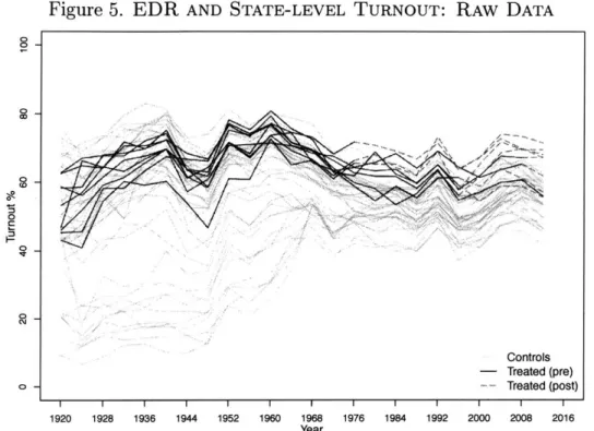
The second chapter examines the effect of Election Day Registration (EDR) laws on voter turnout in the United States. Conventional difference-in-differences approach suggests that EDR laws had almost no impact on voter turnout. Using the generalized synthetic control method, I show that EDR laws increased turnout in early adopting states but not in states that introduced them more recently.

The third chapter investigates the role of informal institutions on the quality of governance in the context of rural China. Using TSCS analysis and a regression discontinuity design, I show that village leaders from large lineage groups are associated with considerably more local public investment. This association is stronger when the groups appeared to be more cohesive. Thesis Supervisor: Teppei Yamamoto

Acknowledgment

It is hard to believe that the six-year long journey at M.I.T. is coming to an end. I still remember the excitement when I first came to Cambridge and visited M.I.T. As I was walking on the bridge connecting E52 and E62, I felt that I was so lucky to able to spend the next five, six years in this place.

Navigating through this journey has not been easy. There is simply too much to learn and there are too many things to choose from. This thesis is not only a collection of work that I have finished at M.I.T., but also represents things I have learned over the years. It would not be possible without the support of my teachers and friends, whom I would like to acknowledge here.

First and foremost, I would like to thank Professor Teppei Yamamoto, Chair of my dissertation committee. It is my honor to be his first official PhD student. Teppei is a great mentor, always caring and thoughtful. He guided me through the last three years of PhD study step by step. He spent hours with me standing in front of a whiteboard, helping me with math problems. He read my papers line by line and gave me suggestions so meticulously that I felt guilty about my sloppiness. He revised the abstract of a paper of mine over and over again and in the end I was amazed how much improvement we had made. I feel much indebted to him. He taught me not only knowledge, but also skills and know-hows required by an independent researcher.

I would like to thank Professor Jens Hainmueller, who has been extraordinarily supportive all the way along. He was very reason I began to think about the main theme of this dissertation and was always there to offer help when I encountered difficulties. Jens genuinely cares about his students and I am very lucky to be one of them. I visited Stanford last year because of him and benefited tremendously from this experience. After I received an invitation for a job interview, Jens checked with me almost everyday, giving me advice and helping me revise every single page of my slides. Working with him was also a lot of fun. I wish one day I could write and communicate as well as he does.

I also wish to thank Professors Lily Tsai and Jim Snyder, who have taught and helped me immensely. Lily was my academic advisor in the first two years. I really appreciate the freedom she gave me in terms of choosing classes and finding a path of my own. Mainly thanks to her, I recognized my huge knowledge gap in the political science literature (and especially in comparative politics). Lily is always there, helping me close that gap. I am still not there yet,

but I will always keep in mind her suggestions. Jim is a scholar I admire even before I came to M.I.T. He convinced me to come to Cambridge and M.I.T. six years ago and I never regretted this choice. The PE breakfast he used to run at M.I.T. was one of the most effective venues in which we learned how to find a good research question, how to design and execute a research project, how to present, and how to criticize each other's work. It was more challenging than most conferences and seminars we later attend.

I would like to thank my friends, teachers, and colleagues, from whom I learned a great deal. I would especially like to thank my coauthors Jennifer Pan and Jidong Chen, who are now professors at leading universities in the U.S. and China, and Professors Devin Caughey and Chris Warshaw at M.I.T., who helped me expand my scope of research. I wish to thank Pro-fessors Danny Hidalgo and In Song Kim, whom I very much enjoy working with as a teaching assistant. I have always benefited from conversations with Professors Yasheng Huang at M.I.T. Sloan and Rod MacFarquhar and Liz Perry at Harvard Government.

Finally, I want to thank my parents for supporting me throughout this journey. You give me everything and I am sorry that I have not been quite around during the past few years.

I will miss this town.

This thesis is supported by a doctoral fellowship provided by the Chiang Ching-kuo Foundation (North America). I thank the Foundation for its professionalism and generosity.

Table of Contents

Introduction

One of the main goals of social science inquiries is to establish causal relationships between real world phenomena. The primary method of establishing causalities is randomized controlled experiments. However, under many circumstances, researchers are unable to conduct experiments because of resource constraints and/or ethical concerns; nor do they always have the opportunity to exploit natural experiments. Previous researches have shown that employing designs with observational, longitudinal data, data of both space and time dimensions, is a promising way to establish causality. This thesis attempts to improve methods of causal inference with time-series cross-sectional (TSCS) data-longitudinal data with many time periods-and apply them to answer important real-world questions.

The core and methodological part of this thesis is what I call the generalized synthetic control method. It unifies fixed effects models, including difference-in-differences (DID), and the synthetic control mothed under a single framework. Specifically, it improves causal inference with TSCS data when treatment units are not randomly selected. Such cases are ample in political science. For example, researchers might be interested in the effect of a reform that took place in several US states, but those states could be funda-mentally different from the rest of the country. Conventional two-way fixed effect models may not be useful when the average treated counterfactual and average control outcome do not follow parallel paths (in which case the so called "parallel trends" assumption fails).

The generalized synthetic control method addresses this challenge. The basic idea is to take into account unobserved time-varying confounders by decomposing the error structure into lower-dimensional factors and conditioning on these factors. It imputes counterfactuals for each treated unit using control group information based on a linear

interactive fixed effect model that incorporates unit-specific intercepts interacted with time-varying coefficients. This method is in the spirit of the original synthetic control method in the sense that, like synthetic control, it uses pre-treatment periods to learn the relationships between treated and control units, based on which it predicts counterfactuals for each treated unit.

This method is widely applicable in political science. For instance, researchers can use this method to estimate the effect a country's joining an international organization on its probability of having conflicts with other countries, or to examine the effect of foreign aid on economic growth. In both cases, we cannot readily assume the parallel trends assumption to be valid. This method has several attractive features. First, because it allows the treatment to be correlated with unobserved unit and time heterogeneities, it is more robust and often more efficient than conventional fixed-effect models. Second, it generalizes the synthetic control method to the case of multiple treated units and variable treatment timing. With this method, users no longer need to find matches for each treated unit since the algorithm produces treated counterfactuals in a single run. Moreover, it addresses the inferential problem of the original synthetic control method and gives more interpretable uncertainty estimates. Finally, with a built-in cross-validation procedure, it avoids specification searches and thus is easy to implement.

The second chapter of this thesis apply the generalized synthetic control method to an empirical application in American politics. Previous researches have not reached a consensus whether Election Day Registration (EDR), a reform meant to reduce the cost of voting, contributed to an increase in voter turnout. The difficulty of causal identification lies in the fact that states that have adopted EDR laws are intrinsically different from those that have not. The two groups of states do not share parallel paths in the pre-EDR law era, suggesting that a DID approach is not a valid identification strategy. Using the new method, I find that EDR laws increased voter turnout in early adopting states, but not in states that introduced EDR as a strategy to opt out the 1993 National

Voter Registration Act or enacted EDR laws in recent years. These results are broadly consistent with evidence provided by a large literature based on individual-level cross-sectional data. They are also more credible than results from conventional fixed effects models when the "parallel trends" assumption appears to fail.

In the third chapter, I apply TSCS analysis to answer an important empirical question in comparative politics: Do informal institutions matter for local governance in envir-onments of weak democratic or bureaucratic institutions? This question is difficult to answer because of challenges in defining and measuring informal institutions and identi-fying their causal effects. In the context of rural China, I investigate the effect of lineage groups on local public goods expenditure. Using a TSCS dataset of 220 Chinese villages from 1986 to 2005, I find that village leaders from the two largest family clans in a vil-lage increased local public investment considerably. This association is stronger when the clans appeared to be more cohesive. I also find that clans helped local leaders over-come the collective action problem of financing public goods, but there is little evidence suggesting that they held local leaders accountable.

Chapter 1

The first chapter of this thesis proposes a new method for causal inference with time-series cross-sectional (TSCS) data, which I call the generalized synthetic control (GSC) method. First, I discuss the literature and provide motivations for developing a new method for causal inference with TSCS data. Then I set up the model and define the main quantity of interest, after which I introduce the GSC estimator and its implementation procedure. The following section discusses the inferential method for the GSC estimator. The last section provides a short summary. Simulation results, additional robustness checks, as well as an empirical example, are provided in the next chapter.

Motivation

Difference-in-differences (DID) is one of the most commonly used empirical designs in today's social sciences. The identifying assumptions for DID include the "parallel trends" assumption, which states that in the absence of the treatment the average outcomes of treated and control units would have followed parallel paths. This assumption is not dir-ectly testable, but researchers have more confidence in its validity when they find that the average outcomes of the treated and control units follow parallel paths in pre-treatment periods. In many cases, however, parallel pre-treatment trends are not supported by data, a clear sign that the "parallel trends" assumption is likely to fail in the post-treatment period as well. This paper attempts to deal with this problem systematically. It proposes a method that estimates the average treatment effect on the treated using time-series cross-sectional (TSCS) data when the "parallel trends" assumption is not likely to hold. The presence of unobserved time-varying confounders causes the failure of this assump-tion. There are broadly two approaches in the literature to deal with this problem. The first one is to condition on pre-treatment observables using matching methods, which may

help balance the influence of potential time-varying confounders between treatment and control groups. For example, Abadie (2005) proposes matching before DID estimations. Although this method is easy to implement, it does not guarantee parallel pre-treatment trends. The synthetic control method proposed by Abaldie, Diamond aiid lairnmuiiieller (2010 9015) goes one step further. It matches both pre-treatment covariates and out-comes between a treated unit and a set of control units and uses pre-treatment periods as criteria for good matches.' Specifically, it constructs a "synthetic control unit" as the counterfactual for the treated unit by reweighting the control units. It provides explicit weights for the control units, thus making the comparison between the treated and syn-thetic control units transparent. However, it only applies to the case of one treated unit

and the uncertainty estimates it offers are not easily interpretable.2

The second approach is to model the unobserved time-varying heterogeneities expli-citly. A widely used strategy is to add in unit-specific linear or quadratic time trends to conventional two-way fixed effects models. By doing so, researchers essentially rely upon a set of alternative identification assumptions that treatment assignment is ignorable conditional on both the fixed effects and the imposed trends (Mora and Reggio 2012). Controlling for these trends, however, often consumes a large number of degrees of free-dom and may not necessarily solve the problem if the underlying confounders are not in forms of the specified trends.

An alternative way is to model unobserved time-varying confounders semi-parametrically. For example, 13ai (2009) proposes an interactive fixed effects (IFE) model, which incorpor-ates unit-specific intercepts interacted with time-varying coefficients. The time-varying coefficients are also referred to as (latent) factors while the unit-specific intercepts are labelled as factor loadings. This approach builds upon an earlier literature on factor 'See isiao. Chiitg and Wan (2012) and Angrist, Jord and Kuersteiiier (201.3) for alternative matching methods along this line of thought.

2

To gauge the uncertainty of the estimated treatment effect, the synthetic control method compares the estimated treatment effect with the "effects" estimated from placebo tests in which the treatment is randomly assigned to a control unit.

models in quantitative fiance." The model is estimated by iteratively conducting a factor analysis of the residuals from a linear model and estimating the linear model that takes into account the influences of a fixed number of most influential factors. Pang (2010, 2(14) explores non-linear IFE models with exogenous covariates in a Bayesian multi-level framework. Stewart (2014) provides a general framework of estimating IFE models based on a Bayesian variational inference algorithm. Gobillon And Mlagnic (2013) show that IFE models out-perform the synthetic control method in DID settings when factor loadings of the treatment and control groups do not share common support."

This paper proposes a generalized synthetic control (GSC) method that links the two approaches and unifies the synthetic control method with linear fixed effects models under a simple framework, of which DID is a special case. It first estimates an IFE model using only the control group data, obtaining a fixed number of latent factors. It then estimates factor loadings for each treated unit by linearly projecting pre-treatment treated outcomes onto the space spanned by these factors. Finally, it imputes treated counterfactuals based on the estimated factors and factor loadings. The main contribution of this paper, hence, is to employ a latent factor approach to address a causal inference problem and provide valid uncertainty estimates under reasonable assumptions.

This method is in the spirit of the synthetic control method in the sense that by es-sence it is a reweighting scheme that takes pre-treatment treated outcomes as benchmarks when choosing weights for control units and uses cross-sectional correlations between treated and control units to predict treated counterfactuals. Unlike the synthetic match-ing method, however, it conducts dimension reduction prior to reweightmatch-ing such that vectors to be reweighted on are smoothed across control units. The method can also be understood as a bias correction procedure for IFE models when the treatment effect is

3_{See Campbell. Lo and NacKinay (1997) for applications of factor models in finance.}

4_{For more empirical applications of the IFE estimator, see Kii. and Oka (2014) and Gaibulloev, Sandler}

heterogeneous across units.s It treats counterfactuals of treated units as missing data and makes out-of-sample predictions for post-treatment treated outcomes based on an IFE model.

This method has several advantages. First, it generalizes the synthetic control method to cases of multiple treated units and/or variable treatment periods. Since the IFE model is estimated only once, treated counterfactuals are obtained in a single run. Users therefore no longer need to find matches of control units for each treated unit one by one.' This makes the algorithm fast and less sensitive to the idiosyncrasies of a small number of observations.

Second, the GSC method produces normal frequentist uncertainty estimates, such as standard errors and confidence intervals, and improves efficiency under correct model specifications. A parametric bootstrap procedure based on simulated treated counterfac-tuals can provide valid inference under reasonable assumptions. Since no observations are discarded from the control group, this method uses more information from the control group and thus is more efficient than the synthetic matching method when the model is correctly specified.

Third, it embeds a cross-validation scheme that selects the number of factors of the IFE model automatically, and thus is easy to implement. One advantage of the DID data structure is that treated observations in pre-treatment periods can naturally serve as a validation dataset for model selection. I show that with sufficient data, the cross-validation procedure can pick up the correct number of factors with high probability, therefore reducing the risks of over-fitting.

'When the treatment effect is heterogeneous (as it is almost always the case), an IFE model that imposes a constant treatment effect assumption gives biased estimates of the average treatment effect because the estimation of the factor space is affected by the heterogeneity in the treatment effect.

6

For examples, Aceiogli et al. (2013), who estimate the effect of Tim Geithner connections on stock market returns, conduct the synthetic control method repeatedly for each connected (treated) firm; D Ib and Zipperer (2015) estimate the effect of minimum wage policies on wage and employment by conducting the method for each of the 29 policy changes. The latter also extend Abadie. DiAmiiond muid Ha IiI1Mle lkr (2010)'s original inferential method to the case of multiple treated units using the mean percentile ranks of the estimated effects.

The GSC method has two main limitations. First, it requires more pre-treatment data than fixed effects estimators. When the number of pre-treatment periods is small, "incidental parameters" can lead to biased estimates of the treatment effects. Second, and perhaps more importantly, modelling assumptions play a heavier role with the GSC method than the original synthetic matching method. For example, if the treated and control units do not share common support in factor loadings, the synthetic matching method may simply fail to construct a synthetic control unit. Since such a problem is obvious to users, the chances that users misuse the method are small. The GSC method, however, will still impute treated counterfactuals based on model extrapolation, which may lead to erroneous conclusions. To safeguard against this risk, diagnostic checks, such as plotting the raw data and fitted values, are crucial.

Framework

Suppose Yit is the outcome of interest of unit i at time t. Let T and C denote the sets of units in treatment and control groups, respectively. The total number of units is N = Ntr + Nc0, where Nt, and Ne0 are the numbers of treated and control units,

respectively. All units are observed for T periods (from time 1 to time T). Let TO,i be the number of pre-treatment periods for unit i, which is first exposed to the treatment at time (To,i + 1) and subsequently observed for qi = T - TO,i periods. Units in the control group are never exposed to the treatment in the observed time span. For notational convenience, I assume that all treated units are first exposed to the treatment at the same time, i.e., TO,i = To and qi = q; variable treatment periods can be easily accommodated. First, we assume that Yit is given by a linear factor model.

Assumption 1 Functional form:

Yit = 6itDit + x't'3 _{+ A'ft + Eit,}

prior to time t and equals 0 otherwise (i.e., Dit = 1 when i C T and t > To and Dit = 0 otherwise).I 6

it is the heterogeneous treatment effect on unit i at time t; xit is a (k x 1)

vector of observed covariates, / = [/3i, ... , /k]' is a (k x 1) vector of unknown parameters,'

ft = [fitI ... , frt]' is an (r x 1) vector of unobserved common factors, Ai = [Al, - - -, Air]' is an (r x 1) vector of unknown factor loadings, and eit represents unobserved idiosyncratic shocks for unit i at time t and has zero mean. Assumption 1 requires that the treated and control units are affected by the same set of factors and the number of factors is fixed during the observed time periods, i.e., no structural breaks are allowed.

The factor component of the model, A'ft = Ailfit + Ai2f2t + -- - + Air frt, takes a linear,

additive form by assumption. In spite of the seemingly restrictive form, it covers a wide range of unobserved heterogeneities. First and foremost, conventional additive unit and time fixed effects are special cases. To see this, if we set

ft

and rewrite Al1 = ai and f2t = t, then Ailf1t + Ai2f2t = ai + t. Moreover, the

term also incorporates cases ranging from unit-specific linear or quadratic time trends to autoregressive components that researchers often control for when analyzing TSCS data."' In general, as long as an unobserved random variable can be decomposed into a multiplicative form, i.e., Uit = ai x bt, it can be absorbed by A'ft while it cannot capture unobserved confounders that are independent across units.

To formalize the notion of causality, I also use the notation from the potential outcomes

7_{Cases in which the treatment switches on and off (or "multiple-treatment-time") can be easily} incor-porated in this framework as long as we impose assumptions on how the treatment affects current and future outcomes. For example, one can assume that the treatment only affect the current outcome but not future outcomes (no carryover effect), as fixed effects models often do. In this paper, I do not impose such assumptions. See Imai and IKimi (2016) for a thorough discussion.

80 is assumed to be constant across space and time mainly for the purpose of fast computation in the frequentist framework. It is a limitation compared with more flexible and increasingly popular random coefficient models in Bayesian multi-level analysis.

'For this reason, additive unit and time fixed effects are not explicitly assumed in the model. A extended model that directly imposes additive two-way fixed effects is discussed in the next section.

10_{In the former case, we can set fit = t and f2t = t}2

; in the latter case, for example, we can rewrite

Yit = pYi,t-i + x'tO + Eit as Yit = Yo - pt + 4'to + vit, in which vit is an AR(1) process and p' and Yio are the unknown factor and factor loadings, respectively. See Gobilloii and Maginac (201.3) for more examples.

framework for causal inference (Neynian 1923; Ruhin 1974; Holland 1986). Let Yt(1) and Yt(O) be the potential outcomes for individual i at time t when Dit = 1 or Dit = 0, respectively. We thus have Yjt(0) =

4/3o

it +

4/3o

The individual treatment effect on treated unit i at time t is therefore 5

it = Yit (1) - Yit (0)

for any i C T,t > To.

We can rewrite the DGP of each unit as:

Y, = Di o 6, + Xj + FAj + EI, i E 1, 2, .. -Nco, Nco + 1, ... , N,

where Y = [Yl, Y2, - - , YT]'; Di = [Da, Di2,*** , DiT]' and 6i = [6 ii2, -- ,6 iT]'

(sym-bol "o" stands for point-wise product); Ei = [Ei, 6i2, - - , i6r]' are (T x 1) vectors; Xi = [Xi, zi2, -* , XiT]' is a (T x k) matrix; and F = [f, f2,-- ,fT]' is a (T x r) matrix.

The control and treated units are subscripted from 1 to Nc0 and from Nc + 1 to N,

respectively. The DGP of a control unit can be expressed as: Y = Xj/ + FAj + Ei, i E

1, 2, - Ne,. Stacking all control units together, we have:

YeO = XcoO + FA'+Esc, (1)

in which Ye, = [Y1, Y2,-.. , YN,,] and Eco = [1, E2, ... , ENeo] are (T x Nco) matrices; Xco is a three dimensional (T x Neo x p) matrix; and Aco = [A1, A2, - - , AN,] ' is a (Ne, x r)

matrix, hence, the products Xc0o and FA' are also (T x Neo) matrices. To identify

/,

and Aco in Equation (1), more constraints are needed. Following Bai (2003, 2009), I add two sets of constraints on the factors and factor loadings: (1) all factor are normalized,

and (2) they are orthogonal to each other, i.e.:

F'F/T = I, and A'OAcO = diagonal. "

"These constraints do not lead to loss of generality because for an arbitrary pair of matrices F and

AcO, we can find an (r x r) invertible matrix A such that (FA)'(FA)/T = Ir and (A- 1Aco)'A- 1Ac is a diagonal matrix. To see this, we can then rewrite A'F as A)F, in which F = FA and Aj = A- 1Aj for

units in both the treatment and control groups such that F and AcO satisfy the above constraints. The

total number of constraints is r2, the dimension of the matrix space where A belongs. It is worth noting that although the original factors F may not be identifiable, the space spanned by F, a r-dimensional subspace of in the T-dimensional space, is identified under the above constraints because for any vector in the subspace spanned by P, it is also in the subspace spanned by the original factors F.

For the moment, the number of factors r is assumed to be known. In the next section, I propose a cross-validation procedure that automates the choice of r.

The main quantity of interest of this paper is the average treatment effect on the treated (ATT) at time t (when t > To):

ATTt,t>To = E[Yit(1) - Yit()|Dit = 1] = E[6it|Dit = 1]. 12

Because Yit(1) is observed for treated units in post-treatment periods, the main object-ive of this paper is to construct counterfactuals for each treated unit in post-treatment periods, i.e., Yit(O) for i E T and t > To. The problem of causal inference indeed turns into a problem of forecasting missing data.'

Assumptions for causal identification. In addition to the functional form assumption (Assumption 1), three assumptions are required for the identification of the quantities of interest. Among them, the assumption of strict exogeneity is the most important.

Assumption 2 Strict exogeneity.

it _L DjsxjsAjfs, Vij,t,s.

Assumption 2 means that the error term of any unit at any time period is independent of treatment assignment, observed covariates, and unobserved cross-sectional and temporal heterogeneities of all units (including itself) at all periods. We call it a strict exogeneity assumption. It implies that treatment assignment is ignorable to potential outcomes after we condition on observed covariates and r orthogonal, unobserved latent factors, i.e.,

{Yi(1), Yt(O)} .L Ditixit, Ai,

ft,

1 2

For a clear and detailed explanation of quantities of interest in TSCS analysis, see l31ackwell and, Glynn (2015). Using their terminology, this paper intends to estimate the Average Treatment History Effect on the Treated given two specific treatment histories: E[Yit(gt) - Yit(q?)Ji,t_1 = at_1] in which a? = (0, ... , 0), ai = (0, . . . , 0, 1, . . . , 1) with To zeros and (t -To) ones indicate the histories of treatment

statuses. I keep the current notation for simplicity.

"The idea of predicting treated counterfactuals in a DID setup is also explored by Broersin et al.

and conditional mean independence, i.e., E[EitIDit, xit, Aj, ft] = E[eitlxit, AX, ft] = 0. Note that because Eit is independent of Di, and xi, for all (t, s), Assumption 2 rules out the possibility that past outcomes may affect future treatments, which is allowed by the so called "sequential exogeneity" assumption."

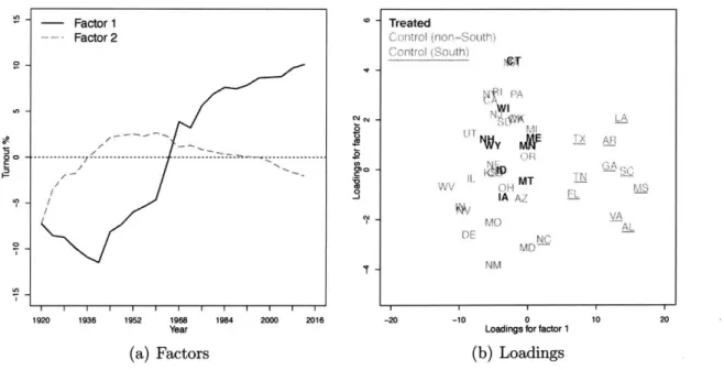
Assumption 2 is arguably weaker than the strict exogeneity assumption required by fixed effects models when decomposable time-varying confounders are at present. These confounders are decomposable if they can take forms of heterogeneous impacts of a com-mon trend or a series of comcom-mon shocks. For instance, suppose a law is passed in a state because the public opinion in that state becomes more liberal. Because changing ideologies are often cross-sectionally correlated across states, a latent factor may be able to capture shifting ideology at the national level; the national shifts may have a larger impact on a state that has a tradition of mass liberalism or has a higher proportion of manufacturing workers than a state that is historically conservative. Controlling for this unobserved confounder, therefore, can alleviate the concern that the passage of the law is endogenous to changing ideology of a state's constituents to a great extent.

When such a confounder exists, with two-ways fixed effects models we need to assume that (Eit + Aift) _LL Djs, xj, aj, I , Vi,

j,

time-varying confounder for unit i at time t, fixed effect for unit

j,

j

Identifying the treatment effects also requires the following assumptions.

Assumption 3 Weak serial dependence of the error terms.

14_{A directed acyclic graph (DAG) representation is provided in the Appendix (Figure 1). See Blackwell}

anid Glynn (2015) and Imai and Kim (2016) for discussions on the difference between the strict ignorability and sequential ignorability assumptions. What is unique here is that we conditional on unobserved factors and factor loadings.

Assumption 4 Regularity conditions.

Assumptions 3 and 4 (see Appendix for details) are needed for the consistent estimation of 3 and the space spanned by F (or F'F/T). Similar, though slightly weaker, assumptions are made in fBai (2009) and Moon and Weidner (2018). Assumption A allows weak serial correlations but rules out strong serial dependence, such as unit root processes; errors of different units are uncorrelated. A sufficient condition for Assumption 3 to hold is that the error terms are not only independent of covariates, factors and factor loadings, but also independent both across units and over time, which is assumed in Aibadie, )iamond

and Ilainmiieller (2010). Assumption 4 specifies moment conditions that ensure the convergence of the estimator.

For valid inference based on a block bootstrap procedure discussed in the next section, we also need to Assumption 5 (see Appendix for details). Heteroskedasticity across time, however, is allowed.

Assumption 5 The error terms are cross-sectionally independent and homoscedastic.

Remark 1: Assumptions 3 and 5 suggest that the error terms Eit can be serially correl-ated. Assumption 2 rules out dynamic models with lagged dependent variables, however, this is mainly for the purpose of simplifying proofs (Bai 2009, p. 1243). As long as the error terms are not serially correlated, the propose method can accommodate dynamic models.

Estimation Strategy

In this section, I first propose a generalized synthetic control (GSC) estimator for treat-ment effect of each treated unit. It is essentially an out-of-sample prediction method based on Bai (2009)'s factor augmented model.

The GSC estimator for the treatment effect on treated unit i at time t is given by the difference between the actual outcome and its estimated counterfactual: 6

-(O), in which Y;t(O) is imputed with three steps. In the first step, we estimate an IFE model using only the control group data and obtain F, F, Ac₀:

Step 1. _{S t e p 1}

(/3,

Z(Y

. ,F ,A co iE C

s.t. 'F/T = I, andXo co = diagonal.

Appendix C explains in detail how such a model is estimated. The second step estimates factor loadings for each treated unit by minimizing the mean squared error of the predicted treated outcome in pre-treatment periods:

Step 2.

A

/3

F

12)

= (F0'F0_)-1_F 0_'(Yi0 _{- XiM),}

i

E

in which / and P0 are from the first-step estimation and the superscripts "0"s denote the pre-treatment periods. In the third step, we calculate treated counterfactuals based on /, F, and

as:

Step 3. Yjt(O) = x't3 +

Z'ft

An estimator for ATT therefore is: ATt =- E T[Yt(l) - Yt(0)] for t > To.

Remark 2: In Appendix E, we show that, under Assumption 1-4, the bias of the GSC shrinks to zero as the sample size grows, i.e. E,(ATTt D, X, A, F) -s ATTt as Nco, To

-0 (Nt, is taken as given)." Intuitively, both large NeO and large To are necessary for the convergences of

/

'5D = [Dj, D2, - - -, DN] is a (T x N) matrix, X is a three dimensional (T x N x p) matrix; and

fixed-effect models.

Model selection. In practice, researchers may have limited knowledge of the exact number of factors to be included in the model. Therefore, I develop a cross-validation procedure to select models before estimating the causal effect. It relies on the control group information as well as information from the treatment group in pre-treatment periods. Algorithm 1 describes the details of this procedure.

Algorithm 1 (Cross-validating the number of factors) A leave-one-out-cross-validation procedure that selects the number of factors takes the following steps:

Step 1. Start with a given number of factors r, estimate an IFE model using the control group data {Yi, Xi}EC, obtaining 4 and F;

Step 2. Start a cross-validation loop that goes through all To pre-treatment periods: a) In round s E {1, - --, To}, hold back data of all treated units at time s.

Run an OLS regression using the rest of the pre-treatment data, obtaining factor loadings for each treated unit i:

Ai,-s = (F'F!8)-F2',(Y0₈ - X9'_,I), Vi E T,

in which the subscripts "-s" stands for all pre-treatment periods except for

S.

b) Predict the treated outcomes at time s using

Y(0)j

+

A',_j

fis(O)

End of the cross-validation loop;

Step 3. Calculate the mean square prediction error (MSPE) given r,

TO

MSPE(r) = e s/To.

s=1 iET

Step 4. Repeat Steps 1-3 with different r's and obtain corresponding MSPEs. Step 5. Choose r* that minimizes the MSPE.

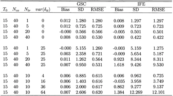
The basic idea of the above procedure is to hold back a small amount of data (e.g. one pre-treatment period of the treatment group) and use the rest of data to predict the held-back information. The algorithm then chooses the model that on average makes the most accurate predictions. A TSCS dataset with a DID data structure allows us to do so because (1) there exists a set of control units that are never exposed to the treatment and therefore can serve as the basis for estimating time-varying factors and (2) the pre-treatment periods of treated units constitute a natural validation set for candidate models. This procedure is computationally inexpensive because with each r, the IFE model is estimated only once (Step 1). Other steps involves merely simple calculations. In the next chapter, we conduct Monte Carlo exercises and show that the above procedure performs well in term of choosing the correct number of factors even with relatively small datasets.

Remark 3: Our framework can also accommodate DGPs that directly incorporate ad-ditive fixed effects, known time trends, and exogenous time-invariant covariates, such as:

Yit= itDit + x13 + -yi'lt + zOt + A'ft + ai + t + Eit, (2)

in which it is a (q x 1) vector of known time trends that may affect each unit differently; -7y is (q x 1) unit-specific unknown parameters; zi is a (m x 1) vector of observed time-invariant covariates; Ot is a (m x 1) vector of unknown parameters; ai and & are additive individual and time fixed effects, respectively." Appendix D describes the estimation procedure of this extended model.

16_{As mentioned in Section , Equation (2) can be represented by the equation specified in Assumption 1} when we set A = y f =, 1 it, A = zi, ft = Ot, A = aj, ft = 1, and A) = 1, fi = (. However, if we know that the model specified in Equation (2) is correct, explicitly including additive fixed effects and time-invariant covariates in the model improves efficiency. Such a model, although requiring more data, relies on an identification assumption that is arguably more appealing than Assumption 2 since time-invariant heterogeneities, universal shocks over time, differential impacts of known time trends, and differential trends caused by observed time-invariant covariates, are all being explicitly conditioned on, i.e., {Yt(1), Yi(0)} _LL Dit 1xit, 1t, zi, aj, t, Aj, ft Vi, t.

Inference

I rely on a parametric bootstrap procedure to obtain the uncertainty estimates of the GSC estimator." When the sample size is large, when Nt, is large in particular, a simple non-parametric bootstrap procedure can provide valid uncertainty estimates. When the sample size is small, especially when Nt, is small, we are unable to approximate the DGP of the treatment group by resampling the data non-parametrically. In this case, we simply lack the information of the joint distribution of (Xi, Ai, 6i) for the treatment group. However, we can obtain uncertainty estimates conditional on observed covariates and unobserved factors and factor loadings using a parametric bootstrap procedure via re-sampling the errors."8 Our goals is to estimate the conditional variance of ATT estimator, i.e.,

Var,(ATTt D, X, A, F) = Var,

(-

Since (Di, Xi, Ai, 6i) are taken as given, the only remaining random variable that is not being conditioned on is Ej, which are assumed to be independent of treatment assignment, observed covariates, factors and factor loadings (Assumption 2). We can interpret Ej as measurement errors or sources of variations in the outcome that we cannot explain but are unrelated to treatment assignment.Y

In the parametric bootstrap procedure, we simulate treated counterfactuals and control units based on the following re-sampling scheme:

1(0) = Xi + FAi + Ei, Vi E C;

Y1(0) =Xz + FAi + E2P, Vi E T.

"Under certain restrictive conditions, such as independent, identically and normally distributed errors, it is possible to derive the analytical asymptotic distribution of the GSC estimator, a necessary step for future research.

18By _{re-sampling entire time-series of error terms, we preserve the serial correlation within the units,}

thus avoiding underestimating the standard errors due to serial correlations (Beck ai1(d l'atz 1995).

19Eit may be correlated with Ai when the errors are serially correlated because )i is estimated using the pre-treatment data.

in which Y' (0) is a vector of simulated treated counterfactuals or control outcomes; Xi3 + FAj is the estimated conditional mean; and Ej and 57 are re-sampled errors for unit i, depending on whether it belongs to the treatment or control group. Ej and 4 are drawn from different empirical distributions because 3 are F are estimated using only the control group information; hence, X43 + FA3 predicts Xj/ + FAj better for a control unit than for a treated unit (as a result, the variance of Ei is usually bigger than that of Ej). Ei is the in-sample error of the IFE model fitted to the control group data, and therefore is drawn from the empirical distribution of the residuals of the IFE model, while ej can be

seen as the prediction error of the IFE model for treated counterfactuals."

Although we cannot observe treated counterfactuals, Yit(0) is observed for all control units. With the assumptions that treated and control units follow the same factor model (Assumption 1) and the error terms are independent and homoscedastic across space (Assumption 5), we can use a cross-validation method to simulate eP based on the control group data (Efroin 2012). Specifically, each time we leave one control unit out (to be taken as a "fake" treat unit) and use the rest of the control units to predict the outcome of left-out unit. The difference between the predicted and observed outcomes is a prediction error of the IFE model. EP is drawn from the empirical distributions of the prediction errors. Under Assumptions 1-5, this procedure provides valid uncertainty estimates for the proposed method without making particular distributional assumptions of the error terms. Algorithm 2 describes the entire procedure in detail.

20_{The treated outcome for unit i, thus can be drawn from Y(1) = Y (0)+6i. We do not directly observe} 6_j,

but since it is taken as given (a set of fixed numbers), its presence will not affect the uncertainty estimates

of ATTt. Hence, in the bootstrap procedure, I use ki(0) for both the treatment and control groups to

form bootstrapped samples (set Ji = 0, for all i E T). We will add back ATTt when constructing confidence intervals.

Algorithm 2 (Inference) A parametric bootstrap procedure that gives the uncertainty estimates of the ATT is described as follows:

Step 1. Start a loop that runs B1 times:

a) In round m e

{1,

},

b) Re-sample the rest of control group with replacement of size Nc, and form

a new sample with one "treated" unit and NeO re-sampled control units; c) Apply the GSC method to the new sample, obtaining a vector of prediction

error;

s(

End of the loop, collecting P = { (2) --- (B 1)

Step 2. Apply the GSC method to the original data, obtaining: (1) ATTt for all t > To, (2) estimated coefficients: 3, F, Aco, and AJJET, and (3) the fitted values and residuals of the control units: Y f = {Y1(O), Y2(0), .. ,

Y

{el, e2, .- , Nc}.

Step 3. Start a bootstrap loop that runs B2 times:

a) In round k E {l, ...

,

i E C (k) = _{Y() +, jET}

in which each vector of ji and 9' are randomly selected from sets e and₃

eP, respectively, and Y(O) = XZ/ + FAi. Note that the simulated treated

counterfactuals do not contain the treatment effect.

b) Apply the GSC method to S(k) and obtain a new ATT estimate; add

(k) ATTt,t>To to it, obtaining the bootstrapped estimate ATTt,t>To.

End of the bootstrap loop.

Step 4. Compute the variance of ATTt,t>T using

1--- (k) B (U) 2

Var(ATTt | D, X, A, F) = k (Ak B = E IAi)t

and its confidence interval using the conventional percentile method (Ekfron an11(d Tibshiranri '1993).

Conclusion

In this chapter, I propose the generalized synthetic control (GSC) method for causal in-ference with TSCS data. It attempts to address the challenge that the "parallel trends" assumption often fails when researchers apply fixed effects models to estimate the causal effect of a certain treatment. The GSC method estimates the individual treatment effect on each treated unit semi-parametrically. Specifically, it imputes treated counterfac-tuals based on a linear interactive fixed effects model that incorporates time-varying coefficients (factors) interacted with unit-specific intercepts (factor loadings). A built-in cross-validation scheme automatically selects the model, reducing the risks of over-fitting. This method is in spirit of the original synthetic control method in that it uses data from pre-treatment periods as benchmarks to customize a re-weighting scheme of control units in order to make the best possible predictions for treated counterfactuals. It generalizes the synthetic control method in two aspects. First, it allows multiple treated units and differential treatment timing. Second, it offers uncertainty estimates, such as standard errors and confidence intervals, that are easy to interpret.

Two caveats are worth emphasizing when applying this method. First, insufficient data (with either a small To or a small Nc0) cause bias in the estimation of the treatment

effect.2 _{Second, excessive extrapolations based on imprecisely estimated factors and} factor loading can lead to erroneous results. To avoid this problem, I recommend the following diagnostics upon using this method: (1) plot raw data of treated and control outcomes as well as imputed counterfactuals and check whether the imputed values are within reasonable intervals; (2) plot estimated factor loadings of both treated and control units and check the overlap.22 When excessive extrapolations appear to happen, we recommend users to include a smaller number of factors or switch back to the conventional DID framework.

21Users _{should be cautious about using this method when To < 10 and N,}

0 < 40.

Appendix: Technical Details

A. A Directed Acyclic Graph (DAG)

Figure 1.. A DAG ILLUSTRATION

I-T0-1 0 IA YTO-1

1

0

00

Note: Unit indices are dropped for simplicity. Vector pt represents unobserved time-varying confounders. If Assumption 1 holds, pt (or pit) can be expressed as A'ft. We allow Di to be correlated with xi,,,<t and pis,,<t. In fact, we also allow it to be correlated with xj2,,<t and pjs,,<t when

j

B. Technical Assumptions

Assumptions 3-5 are shown below.

Assumption 3 Weak serial dependence of the error terms:

1. E(Ei tE ) = o-i,ts, Jo-i,ts 15 &j for all (t, s) such that 1 E 5 M.

2. For every (t, s), EIN- 1/2 _Z:

1[eiseit - E(Ei8Eit)]I4 < M.

3. T2N Ethy u~ EijIcov (Eitsis, EjuEjv)| ZtSuvZ o(~~~ jlKMadTN M and -coeis, 2 Et's Zi,j,k,l 1COV(FitEjt, EkElsih8)I

M.

4. E(Eitsj,) = 0, for all i f j, (t, s).

Assumption 4 Regularity conditions: 1. Elet 18 < M.

2. E||xit|14 _{< M: Let = {F:F'F/T = I}. We assume infFEF D(F)}

which D(F) =

I

A' (A' oAco)

Ak-3. El|ft|1 4 K M < oo and j E 1ftft' 4 EF for some r x r positive definite matrix

EF, as T0 -+ oc.

4. Ej|Ai 14 K M < oc and A'OAcO/No 4 EN for some r x r positive definite matrix EN, as Nc, -- oc.

Assumption 5 The error terms are cross-sectionally independent and homoscedastic. 1. eit _LL Ej, for all j # i, (t, s).

2. E(ejtEi8) = o-t, M, for all (t, s).

C. Estimating an Interactive Fixed-effect Model

As in Equation (1), I assume that the control units follow an interactive fixed-effect model:

YeO = Xco# + FA' + Eco,

The least square objective function is

Neo

SSR(O, F, Aco) = (Yi - XiO - FAi)'(Y - Xi/ - FAi).

i=1

The goal is to estimate

/,

F'F/T = I, and A' Aco = diagonal.

A unique solution (3, F, Aco) to this problem exists. To find the solution, Bai (2009) proposed an iteration scheme that can lead to the unique solution starting from some initial value of

/

NcO- NcO

#(F, A) = Xi~ X X '(Y - F,\ ),

and given

#,

+ i:

[NT - c(Y- Xi3)(Y - X /)']F = FVNOT,

Ac=

}(Y

in which VNcoT is a diagonal matrix that consists for the first r largest eigenvalues of the

(Nc, x Ne,) matrix N _' (Y - Xi/)(Y - Xi /)' and VNeOT = coA co

N~No 0

D. Estimation Procedure for an Extended Model

Without loss of generality, we re-write Equation (2) as

Yit= &Dit + x/t3 + -yi'lt + z,&t + A'ft + ai + t + p + Eit,

in which p is the mean of control group outcomes, which allows us to impose two re-strictions: EN ai = 0 and E *O = 0. As before, we use three steps to impute the counterfactuals for treated units. It can be written as

Y = 6, o Di + X,3+ L7 + Oz, + Fhi + ailT + + + T +Ei,

in which L = [11, 12,- iT]', a (T x q) matrix;

e

and E = [ 2, - - - , T]', a (T x 1) vector. In the first step, we estimate an extended IFE

model using only the control group data and obtain /,F,Ao, B,

E,

Step 1. 01 _, 6, $, CO, {$}, {ai}, = argmin E EIjj. iEC

in which ej = Y - X43 - Lie- (zi - FAi - &i1T -- - lT. The details of the estimation strategy can be found in Bai (2009) Sections 8 and 10.

The second step estimates factor loadings, as well as additive unit fixed effects, for each treated unit by minimizing the mean squared error of the treated units in the pre-treatment period:

Step 2. i i) = _{argmin e'ei}

(ii A. &i)'

=

(G'

)-1

[LT

),

in which ei = Y0 - X? - Lo0I - O0zi - 0 AI - di - &? - f;

3,

E,

matrix.

In the third step, we calculate the counterfactual based on

/,

+,

E. Proofs of Main Results

I use the Frobenius norm throughout this paper, i.e., for any vector or matrix M, its norm is defined as ||M|| = /tr(M'M). I establish four lemmas before getting to the main results.

Lemma 3 (i) T-1/2 I P0 I = 0,(1); (ii) T (F01' 0)-1|1 = 0,(1). Proof: (i). Because tr(F'F/T) = r,

T- -Poll T- 2 tr( 0 0) < T 1

/2 tr(F'F) = Vr.

(ii). Denote

Q

||ftf'll = 0,(1) and there are only qj items in the summation,

11Q11

O(1).

Q

(P

_Q

Since

Q

Lemma 4 |j3 - 011 = Op(Nc1) + Op(T-1)+o

((NcoT)

Proof: Bai (2009) shows that under Assumptions 3 and 4. and when T/N2 -+ 0:

/ - / =D(F)- 1 NCO E[XIMF 1 1 1 + N _{Nco T} (-+ o/NT_pNc where D(F) Nc0T NCO Z , NCO - 11:aikXkMF]Ei MFXi - - MFXkaik, NCO k=1 1 _A'cOAC Nco (X- Vj'F FF T (T )

)

1_{Ak, V a X , Q= - Ec" E(ekE' ). Therefore, /} (3) NCO Nco -D(P)- 1 _ i=1 k=1

and aik - ' AO/Nco)

is an asymptotically unbiased estimator for 3 when both T and Nc, are large and

I!/11,3

/2)

Lemma 5

Denote H =

(AVAc)

(i). ||ft - H-1ft|| = C + Op(T 1/2

(ii). |ift - ft'( fO/0)-1'oIFI = -1/2) + Op(T- 1_/2₎

Proof: (i). The main logic of this proof follows Bai (2009) Proposition A.1 (p. Because

NeO

-(Yi Xi)(Y - ') F = FVNoT

and Yj - Xj/ = Xt(/3 -

f)

have: .VNCOT =NT No +NcoT E=

(03

/3)(/

3)'X,

ZEiAF'F

with the last term on the right-hand side equal to NT c* FA A'F'F. Denote G = 1

ENT

+ F

J