Less is more : efficient hardware design through Approximate Logic Synthesis

(1)

through Approximate Logic Synthesis

Doctoral Dissertation submitted to the

Faculty of Informatics of the Università della Svizzera Italiana in partial fulfillment of the requirements for the degree of

Doctor of Philosophy

presented by

Ilaria Scarabottolo

under the supervision of

Prof. Laura Pozzi

(2)

(3)

Prof. George A. Constantinides Imperial College London, United Kingdom Prof. Jörg Henkel Karlsruhe Institute of Technology, Germany Prof. Akash Kumar Technische Universität Dresden, Germany Prof. Cesare Alippi Università della Svizzera italiana, Switzerland Prof. Antonio Carzaniga Università della Svizzera italiana, Switzerland Prof. Laura Pozzi Università della Svizzera italiana, Switzerland

Dissertation accepted on 15 October 2020

Research Advisor PhD Program Director

Prof. Laura Pozzi Prof. Walter Binder, Prof. Silvia Santini

(4)

ted previously, in whole or in part, to qualify for any other academic award; and the content of the thesis is the result of work which has been carried out since the official commencement date of the approved research program.

Ilaria Scarabottolo

Lugano, 15 October 2020

(5)

remains to be done.

Marie Curie

(6)

(7)

As energy efficiency becomes a crucial concern in almost every kind of digital application, Approximate Computing gains popularity as a potential answer to this ever-growing energy quest.

Approximate Computing is a design paradigm particularly suited for error-resilient applications, where small losses in accuracy do not represent a signifi-cant reduction in the quality of the result. In these scenarios, energy consump-tion and resources employment (such as electric power, or circuit area) can be significantly improved at the expense of a slight reduction in output accuracy.

While Approximate Computing can be applied at different levels, my research focuses on the design of approximate hardware. In particular, my work explores Approximate Logic Synthesis, where the hardware functionality is automatically tuned to obtain more efficient counterparts, while always controlling the entailed error. Functional modifications include, among others, removal or substitution of gates and signals. A fundamental prerequisite for the application of these modifications is an accurate error model of the circuit under exam.

My Ph.D. research work has deeply concentrated on the derivation of ac-curate error models of a circuit. These can, in turn, guide Approximate Logic Synthesis algorithms to optimal solutions and avoid expensive, time-consuming simulations. A precise error model allows to fully explore the design space and, potentially, adjust the desired level of accuracy even at runtime. I have also contributed to the state of the art in ALS techniques by devising a circuit pruning algorithm that produces efficient approximate circuits for given error constraints. The innovative aspect of my work is that it exploits circuit topology and graph partitioning to identify circuit portions that impact to a smaller extent on the final output. With this information, ALS algorithms can improve their efficiency by acting first on those less-influent portions. Indeed, this error characterisation proves to be very effective in guiding and modeling approximate synthesis.

(8)

(9)

This thesis is the result of several years of work, although technical research rep-resents only a small fraction of it. These have been years of excitement, learning, self-questioning, doubts about the future, pride, and great personal development. I cannot start but from thanking my research advisor Prof. Laura Pozzi, who has been much more than that throughout these years. Thank you Laura, for all your precious advice, your ever-present support and your motivation in pursu-ing my objectives. What I’d like to thank you most for, though, is the constant reminder you gave me on my professional and personal value, and on the impor-tance of acknowledging it.

I often joke about the fact that I’d have never earned a Ph.D. without Dr. Lorenzo Ferretti, and I wonder how far this is from reality. Thank you Lorenzo for always being willing to help me with my endless questions, and for all the fun time we have spent together.

I will never thank my family enough for the unconditional support they have always given me since my earliest days, and which of course did not fade for a second during these past few years.

Finally, I’d like to thank all my closest friends. Thank you for all the joy and laughter, for reminding me that no problem is as tough as it seems, and for celebrating this great milestone like no other.

(10)

(11)

Contents ix

List of Figures xi

List of Tables xiii

1 What is Approximate Computing? 1

1.1 Approximate circuits . . . 3

1.2 Approximate Computing potential: a case study for multiple ap-proximation levels . . . 4

2 Approximate Logic Synthesis: algorithm categorization and error mod-eling 7 2.1 ALS algorithms . . . 7

2.1.1 ALS structural netlist transformation . . . 10

2.1.2 ALS logic rewriting based methods . . . 13

2.2 Error modeling for guiding ALS . . . 15

2.2.1 Error Metrics . . . 17

2.2.2 Methods for Error Modeling . . . 20

3 Circuit Carving: exhaustively exploring approximations 23 3.1 Introduction . . . 23

3.2 Problem formulation . . . 24

3.2.1 Exploration Algorithm . . . 25

3.2.2 Error modeling . . . 27

3.3 Experimental evaluation . . . 29

3.3.1 Performance of inexact circuits . . . 29

3.3.2 Effectiveness of Search Space Pruning . . . 30 ix

(12)

4 A formal framework for error modeling 33

4.1 Error model formal definition . . . 34

4.2 P&P-Monotonicity . . . 38

4.2.1 Propagation mechanism . . . 39

4.2.2 Non-monotonic outputs . . . 41

4.2.3 Non-strict monotonic outputs . . . 42

4.2.4 Final error model derivation . . . 43

4.3 P&P-Intervals . . . 43

4.3.1 Primary output intervals . . . 44

4.3.2 Input interval derivation and propagation . . . 45

4.4 Sum propagation . . . 48

4.5 Graph partitioning . . . 49

4.5.1 Time complexity analysis . . . 51

4.6 Performance of the proposed algorithms . . . 52

4.6.1 P&P-Intervals values Ii . . . 53

4.6.2 Weight values comparison . . . 54

4.6.3 Online adders . . . 57

4.6.4 Faster vs slower circuits . . . 57

4.6.5 Maximum number of inputs per subgraph . . . 60

4.7 Effectiveness of error modeling for ALS . . . 61

5 Dealing with expected error 65 5.1 Problem definition . . . 65

5.2 Maximum error propagation . . . 68

5.3 Average error propagation . . . 69

5.4 Preliminary results and comparisons . . . 70

6 Achievements and future work 75 6.1 Publications . . . 75

6.2 Ongoing research . . . 76

6.2.1 Collaborations with Prof. S. Reda . . . 76

6.2.2 Exploiting the primary inputs characteristics . . . 77

6.2.3 Re-thinking partitioning . . . 78

6.2.4 Approximate Neural Networks . . . 79

6.2.5 Circuit Carving reformulation: heuristics for scalability . . 79

(13)

1.1 Approximate Computing taxonomy. . . 2

2.1 Approximate Logic Synthesis techniques: main categories. . . 8

2.2 Common ALS flow in the state of the art. . . 9

2.3 GLP[1] algorithm. . . 11

2.4 SASIMI[2] algorithm. . . 12

2.5 SALSA[3] algorithm. . . 13

2.6 BLASYS[4] algorithm. . . 15

2.7 Error modeling for ALS. . . 17

2.8 EDAP reduction in an 8-bit multiplier. . . 18

3.1 Circuit Carving definition. . . 25

3.2 Closure of a cut. . . 26

3.3 A full-adder labelled with its weights. . . 28

3.4 Weight propagation in a ripple-carry adder. . . 29

3.5 EDAP reduction for CC vs GLP. . . 31

3.6 Effect of pruning criteria on the number of recursive calls. . . 32

4.1 Strengths and weaknesses of SoA in error modeling. . . 34

4.2 Partition and Propagate method description. . . 35

4.3 Approximate circuits with gate outputs set to a constant. . . 36

4.4 Label propagation model. . . 37

4.5 P&P subsumes multiple error modeling strategies. . . 38

4.6 Propagation matrix derivation. . . 40

4.7 Non-monotonic output bits propagation. . . 41

4.8 Non-strict monotonic output bits propagation. . . 42

4.9 PO intervals assignment for a ripple-carry adder. . . 44

4.10 Interval computation for the inputs of a generic subgraph. . . 46

4.11 Detailed computation of Figure 4.10a. . . 46

4.12 External fan-outs in partitioning. . . 47 xi

(14)

4.13 Sum propagation in a DAG. . . 49

4.14 Extreme partitions. . . 50

4.15 Two-phase partitioning. . . 51

4.16 Intervals and weights retrieved by PP-Int. . . 54

4.17 Weight comparison in small benchmarks. . . 55

4.18 Weights comparison in adders, multipliers and euclidean distance. 56 4.19 Weights comparison for online adders. . . 58

4.20 Weights comparison for SAD with different delay constraints. . . . 59

4.21 Effect of maximum number of inputs per subgraph on weights. . . 61

4.22 EDAP reduction for GLP guided by sum propagation or PP-Mon. . 63

5.1 Gate outputs set to a constant, as in Figure 4.3. . . 66

5.2 Label propagation model, as in Figure 4.4. . . 67

5.3 Interval computation for expected error. . . 68

5.4 Expected weights forADDER8. . . 71

5.5 Expected weights forMULT8. . . 72

(15)

2.1 Summary of the ALS works described, where NT stands for Netlist Transformation, and BR for Boolean Rewriting. . . 16 4.1 Summary of the three algorithms subsumed by the Partition and

Propagate framework. . . 48 4.2 Characteristics of Benchmarks employed in[5]. . . 53 4.3 Influence of threshold T on resulting partitions, in terms of

num-ber of resulting subgraphs, infeasible subgraph ratio, and average distance from exact weights (when available). . . 60 5.1 Accuracy of the proposed methods against Monte Carlo

Simula-tion onADDER8. . . 71

5.2 Accuracy of the proposed methods against Monte Carlo Simula-tion onMULT8. . . 73

(16)

(17)

What is Approximate Computing?

Technology has now manifestly become a pervasive aspect of social, industrial and economical life. The constant growth of the amount of data exchanged, the energy required to maintain IT services and the astonishing diffusion of mobile devices require a fast and reactive performance improvement on one side, and highlight challenging issues regarding energy supply on the other. Indeed, en-ergy efficiency should nowadays be regarded as a most crucial concern in every kind of application.

At the same time, several energy-hungry applications are gaining so much popularity that their role is becoming fundamental in shaping our society, and their environmental impact cannot be ignored. Some examples are image pro-cessing, machine learning, robotics, wireless sensor networks and, in general, digital signal processing. In traditional computing, exactness of result has al-ways been a cornerstone, but this exactness is not needed anymore in most of these applications; nonetheless, today these are still implemented on platforms and accelerators born under the traditional paradigm of full precision and relia-bility.

Approximate Computing (AC) represents a valid instrument to answer the constantly growing need for high performance at low energy cost of error-resilient applications, since it can lead to substantial energy savings in exchange for small losses in the output quality. As a simple example, in image processing a small quality loss in digital pictures cannot even be perceived by human eyes. The key idea under Approximate Computing is to relax requirements on exactness, in favour of improved energy efficiency, which in turn manifests in reduced hard-ware area and resource employment, or faster execution time.

Thanks to the growing diffusion of error-resilient applications, research in Approximate Computing has flourished in the past few years, spanning through

(18)

Functional simplification latency area/power accuracy (a) (b) (c) Approximate software Approximate architecture Approximate circuit AC Voltage overscaling

Figure 1.1. (a) Accuracy represents a new dimension for circuit synthesis . (b) Approximate Computing (AC) techniques taxonomy. (c) A simple example of functional approximation for circuits: some gates, along with their wired connections, are removed from the original circuit (above), resulting in a smaller inexact circuit (below).

different levels of the hardware/software stack [6, 7]. A first, rough division of AC techniques is represented by the three main categories of Figure 1.1b: approximate software development, approximate architecture exploration, and approximate circuit design[8].

An example of software, or program-level approximation[9,10] is loop perfo-ration[11], where some iterations of a loop are skipped, either deterministically or randomly; the degree of perforation influences the accuracy of the final result. Another example belonging to the same category is thread fusion, where differ-ent threads are combined by merging two dynamic instances of the same static instruction into a single one[12]. Pattern reduction [13] is yet another possibil-ity: here, different patterns which are usually found in parallel programs, such as map or reduction, are identified and associated with a specific approximation to optimise the overall performance.

At the architectural level, approximate storage and processors may be em-ployed. Approximate processors architectures can either run traditional code on a processor designed to execute some specific instructions in approximate mode, or turn approximable segments of traditional code into a neurally in-spired algorithm running on accelerators. In both cases, a compiler or manual intervention by a programmer are necessary to annotate approximable code seg-ments [14, 15]. Memory and storage can also be exploited to trade accuracy for performance[16–18] by relaxing the requirements on storage precision,

(19)

protec-tion from particle strikes or RAM energy supply.

Finally, in approximate circuits, hardware is intrinsically designed to compute inexact operations. My research focuses on this level of approximation, which is further detailed in the next section.

1.1 Approximate circuits

Traditionally, circuit design has adopted several strategies to balance the trade-off existing between area (or power) and latency. Quicker circuits can hardly be obtained without increasing their size and their global power consumption. Approximate Computing adds a third dimension to the area-latency trade-off: the accuracy of the circuit output (Figure 1.1a), offering a substantial number of new possibilities to designers and engineers struggling with their demanding requirements.

The large family of approximate circuit design techniques can be divided into the two subcategories of Figure 1.1b: overscaling and functional. Overscaling aims at lowering a circuit supply voltage without reducing the corresponding op-erational frequency, thus reducing its static and dynamic energy while inducing timing errors [14, 19, 20]. However, these timing errors may result in uncon-trollably large computational errors, limiting the usability of these solutions[8]. Workaround to this problem are redesign techniques, such as the ones proposed in[21], or careful considerations on the statistical distribution of inputs [22].

In functional approximation, instead, the original boolean function executed by a circuit is modified with the purpose of trading accuracy for performance. Figure 1.1c illustrates a simple example: some gates of a generic circuit are cut to obtain an approximate version, which will compute erroneous values for a subset of the circuit inputs. If this error is limited, and can be tolerated by the application of interest, the original circuit can be replaced by its smaller, more efficient approximate version[1,23].

Many approaches belonging to this category focus on the design of specific approximate arithmetic units, e.g. adders [24–29], multipliers [30–35], or di-viders[36–38]. Other works [39, 40] present algorithms that allow to automat-ically explore the energy-quality trade-off, but again limit the analysis to adders and multipliers only. Unlike these hand-crafted or circuit-specific designs, many research contributions developed wider-scope generic approximate circuit design techniques, that can be applied to any logic circuit without a-priori knowledge of its functionality[2–5,23,41–44]; my research work also belongs to this latter category.

(20)

Moreover, these circuits constitute the basic building blocks for large-scale applications[45–47] such as, for instance, neural networks [48–51], and several works study how the error can be distributed [52] or can propagate [53–57] among different approximate circuits in a larger system.

1.2 Approximate Computing potential: a case study for

multiple approximation levels

In Agrawal et al.[58] the authors explore the combined effect of approximations introduced at different levels, in order to demonstrate the potential of Approxi-mate Computing in enhancing the performance of error-resilient applications.

To represent different approximation levels, the authors chose to apply simul-taneously loop perforation, reduced arithmetic precision and relaxation of thread synchronisation. In reduced precision, variables and data structures of a program are represented with fewer bits than the original integer or floating point repre-sentation, allowing to employ smaller circuits and, hence, using cheaper and less consuming hardware. Thread synchronisation instead is employed to guarantee that different threads reach execution checkpoints in a predictable manner, or share the correct values of global variables; however, synchronisation can be sys-tematically relaxed to improve performance.

The three above mentioned approximation techniques are applied to common image processing applications, such as Synthetic Aperture Radar (SAR) and Wide Area Motion Imagery (WAMI), or commonly used machine learning techniques, such as K-means Clustering and Deep Neural Networks, and, finally, Robot Lo-calization.

Their results confirm and validate the interest in Approximate Computing: indeed, without loss of accuracy (which means detecting the correct objects in image recognition, or identifying the same clusters in K-means), they were able to perforate hot loops with an average factor of 50%, with a proportional decrease of the execution time. Moreover, data bit width was reduced from 32 or even 64 bits to a range of 10 – 16 bits. As for parallel applications, they were able to halve the execution time through relaxed synchronisation. However, the most important result is that concurrent application of these three techniques further improved the overall performance.

Their conclusion, which I strongly agree with, is that "As the benefits of

ap-proximate computing are not restricted to a small class of applications, these results motivate a re-thinking of the general purpose processor architecture to natively

(21)

sup-port different kinds of approximation to better realise the potential of approximate computing.".

My PhD research work has focused on approximations at hardware level, al-ways with a view to a subsequent integration in larger systems, where potentials of approximations are exploited at all levels. Indeed, works as [58] further en-courage research in approximate hardware synthesis, since they prove that no level has more potential than the others, but rather the wise combination of ap-proximations may represent a key to sustainable development.

(22)

(23)

Approximate Logic Synthesis: algorithm

categorization and error modeling

Given an intended functionality, established methodologies for hardware de-sign focus on achieving good trade-offs between performance metrics (e.g. la-tency, throughput) and cost (energy and resource requirements). Hence, higher-performance circuits can only be obtained by increasing their size or power bud-get, while the relationship between inputs and output values is kept invariant. Approximate Logic Synthesis (ALS) expands the scope of this process by adding an extra dimension to the design space of possible solutions: that of the tolerated implementation inaccuracy. ALS, indeed, indicates the process of synthesising in-exact hardware starting from an in-exact Boolean formulation.

Approximate hardware components realized with ALS can, at the same time, offer remarkable gains in area and efficiency and significant performance in-creases with respect to their exact counterparts, in exchange for small losses in output quality. ALS is hence the embodiment, at the hardware design level, of Approximate Computing (AC). Approximate circuit synthesis is particularly attractive since approximate circuits are employed as basic blocks for realizing application-specific accelerators, which are a highly relevant component of mod-ern Systems-on-Chips[59].

The large family of algorithms that functionally modify a circuit are reunited under the domain of Approximate Logic Synthesis (ALS).

2.1 ALS algorithms

The transformation of a generic Boolean function f into its approximate coun-terpart ˜f can be performed in different ways.

(24)

i_n ... i₀ o₁o₀ 0 0 ... 0 0 0 ... 1 ... 1 1 ... 0 1 1 ... 1 0 1 1 1 ... 1 0 0 1 in ... i0 o1 o0 0 0 ... 0 0 0 ... 1 ... 1 1 ... 0 1 1 ... 1 0 0 0 1 ... 1 0 1 1 module C(o1,..,in);

...

assign o1 = a + b

assign o2 = a * b

... endmodule

module C(o1,..,in);

... assign o1= a | b assign o2= a * b ... endmodule

(a)

(b)

(c)

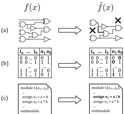
Figure 2.1. Possible functional simplification approaches are illustrated: a generic Boolean function f is transformed into ˜f , either acting on a

synthe-sised netlist, for instance at gate-level (a), or on its truth table (b). Finally, the circuit at behavioural level can be simplified by approximate high-level synthesis (c).

Three main classes can be identified for such approaches, illustrated in Figure 2.1: Netlist transformation, Boolean rewriting and Approximate high-level

synthe-sis.

In Netlist transformation (Figure 2.1.a), the Boolean function f is already mapped into a netlist, i.e., a list of components such as Boolean gates imple-menting simple functions, for instance AND,ORandNOT. Approaches belonging to this category start from these netlists, and transform them by removing some nodes, or by substituting some wires with others, hence reducing the circuit size and power consumption. My research work has focused on this category of tech-niques.

Boolean rewriting approaches act on the function truth table, which repre-sents a higher level of abstraction: no choice of employed electrical components has been made yet, only the list of input combinations of f and the corresponding outputs is available. Therefore, this description is independent from the netlist

(25)

approximate design exact design QoR evaluation ALS method

Figure 2.2. Common ALS flow in the state of the art: after the application of an ALS method, the approximate circuit is evaluated to verify that the induced error does not exceed the predefined limit. The result of this test is the final approximate design.

selected to implement the function, generating a specific circuit. Methods be-longing to this category, illustrated in section 2.1.2, modify the values of such outputs for a subset of the input combinations, as illustrated in Figure 2.1.b: in the output columns, some values in bold have been flipped w.r.t. the original truth table.

Finally, Approximate high-level synthesis focuses on the highest level of ab-straction for ALS, where the function is described at behavioural level, such as in RTL Verilog or C language. An example fragment of such code is depicted in Figure 2.1.c, where a portion of C code shows how output values are computed from the function inputs by providing a mathematical expression, instead of list-ing all possible input combinations. These functions can be approximated as in the example, where the sum is transformed into a logicalOR.

Independently from the approach chosen among those described above, the process of synthesizing an approximate circuit is exemplified in Figure 2.2: an ALS method is applied to the exact design, leading to a smaller – and more effi-cient – circuit. In the simple example of the figure, representing a netlist trans-formation approach, two gates are removed from the circuit. Before obtaining the final approximate design, a QoR evaluation phase is necessary: the circuit needs to be tested in order to verify that the error does not exceed the tolerated limit. We will see that an earlier error modeling phase is fundamental for pre-dicting the effect of functional transformations and guide ALS methods: such preliminary step represents a major focus of my work.

The next sections report the principal works in the state of the art for the two first algorithm classes of Figure 2.1, namely netlist transformation and Boolean rewriting. Approximate high-level synthesis, instead, will not be further investi-gated, since its higher level of abstraction makes it less relevant in the discussion of this thesis.

(26)

2.1.1 ALS structural netlist transformation

Among methods that implement structural netlist transformation, three main categories can be distinguished: greedy heuristics, stochastic netlist transforma-tions, and exhaustive exploration.

Shin et al. [60] employ a greedy strategy for generic circuit simplification, where a set of stuck-at-faults are injected in the circuit, and a heuristic is em-ployed to iteratively choose the SAF that maximizes a given figure of merit (e.g., area reduction), simplify the circuit forward and backward, and repeat the pro-cess until the error constraint is violated.

GLP by Schlachter et al.[1] presents another greedy iterative algorithm for circuit simplification. The proposed framework, depicted in Figure 2.3, is simple but effective. The exact circuit is represented as a direct acyclic graph and nodes are pruned according to two main criteria: the node significance, which repre-sents the impact of that node on the final output, and the node activity or toggle count. According to the application characteristics, nodes can be pruned starting from those with lower significance, lower activity, or a combination of the two: the significance-activity product (SAP). Node activity is obtained through gate-level hardware simulation, while significance is computed in a reverse topologi-cal graph traversal, starting from the primary outputs arithmetic bit-significance, then assigning to each node i the significanceσ_i:

σi=X σd esc(i),

where d esc(i) are all direct descendants of node i.

After nodes have been ranked according to the desired metric, the GLP frame-work iteratively removes a node from the original circuit, setting its output to a constant; it then resynthesizes the circuit and simulates it with a Monte Carlo process to verify that the error constraints on error rate and mean relative error have not been violated. This, indeed, represents the QoR validation phase de-picted in Figure 2.2. After each iteration of gate removal, GLP recomputes SAP for node ranking, until the error threshold is reached.

Computing node activity can take a considerable amount of time (15 to 20 minutes for a 32-bit adder with 5 million input combinations). However, it allows the selection between a wider range of performance-accuracy trade-offs for the same amount of tolerated error. Therefore, significance-only node ranking is preferred for a first, fast design, while SAP ranking can be employed for fine tuning.

(27)

remove one gate from the circuit

simulate the obtained circuit error threshold reached? YES Approximate circuit NO 1 2 4 8 16 1 3 4 4 12 16 15 28

Figure 2.3. GLP [1] framework. Gates are removed from a generic circuit starting from the least significant, until the allowed error threshold is reached.

Venkataramani et al.[2] propose another greedy strategy called SASIMI (Sub-stitute And SIMplIfy). In SASIMI, functional approximation is performed by iden-tifying pairs of signals that assume the same value with high probability, and substitute one with the other. When the target signal is replaced, the gates be-longing exclusively to its generating cone of logic are removed from the circuit, while others can be downsized, as illustrated in Figure 2.4. Clearly, the error in-duced by a potential substitution must be considered in the choice of the target signal. This error can be estimated through a Monte Carlo process that assess the error rate and average absolute error magnitude on a subset of all possible circuit inputs, which are assumed to be uniformly distributed. The algorithm takes as input the original circuit and a target error, then iteratively performs the selection of the best candidate signal pair, the substitution and consequent circuit simplification, followed by QoR evaluation. Once the target error constraint is reached, the iterative algorithm stops.

Liu et al. [61] argue that the assumption of uniform distribution of input data is seldom correct. Therefore, they propose SCALS: Statistically Certified Approximate Logic Synthesis, an iterative framework where statistical hypothe-sis testing is employed to estimate the errors obtained on the circuit outputs after an approximate transformation. This approach guarantees that the population behaviour is indeed a faithful representation of the actual data distribution. In SCALS, the transformation space is explored stochastically, which means consid-ering possible transformations at random, instead of employing fixed heuristics, so as to maximize the number of design points tackled.

(28)

TS SS pri m ary input s pri m ary out put s

original circuit

pri m ary input s pri m ary out put s

approximate circuit

SS pruned gates down-sized gates

Figure 2.4. In SASIMI [2], a target signal (TS) is substituted with another circuit signal (SS). Gates belonging to TS cone of logic are either removed or downsized.

In a similar direction, Vasicek and Sekanina propose EvoApprox, a genetic al-gorithm to mutate the circuit into approximate versions by swapping gates with wire connections[62]. Circuits are represented as direct acyclic graphs, whose nodes can be Boolean gates or more complex components according to the tech-nology library chosen. The nodes are contained in a two-dimensions grid, the

chromosome, which is randomly modified to explore new design points. This

mutation evolves using a fitness function, which leads to better approximation over runtime. After computing area and error of the initial population, the al-gorithm iteratively selects the best-scored circuit, generatesλ offspring from the parent through mutation, and evaluates the new population. To evaluate the error obtained at each mutation, full-simulation is employed for small circuits, while for larger circuits the authors resort to more complex techniques such as SAT or BDD-based evaluation.

Using And-Inverter-Graphs as the circuit representation, Chandrasekharan et

al.[63] propose an algorithm for approximate AIG re-writing that guarantees the

bounds of approximation errors introduced in the approximate circuit. First, the critical paths are identified in the AIG, where the critical paths are the paths from the primary inputs to the primary outputs with the largest number of nodes. After this step, cut enumeration on the selected paths is used to identify potential cuts. A SAT solver is then employed to compare the original AIG and the approximate AIGs to check wether the error constraint is violated, hence guaranteeing the error bound.

As opposed to other works surveyed in this section, Circuit Carving[23] does not employ iterative approximations towards inexact logic synthesis. It instead resorts to exhaustive exploration of all possible nodes subsets that can be

(29)

re-inputs accurate outputs approximate outputs

i

1

, . . . , i

n 1/0 original circuit approximate circuit QoR ~

Figure 2.5. In SALSA a QoR circuit is constructed to compare the outputs of exact and approximate circuits [3]. Observabilitydon’t cares of the approximate

circuit are used to minimize the approximate circuit logic.

moved from the exact circuit, among which the most convenient will be chosen. The best candidate sub-circuit is the largest one (in terms of number of gates) that does not overcome the identified error threshold. This latter work will be described in detail in Chapter 3.

2.1.2 ALS logic rewriting based methods

ALS using Boolean rewriting can be categorized as a general approach in which the logic of the circuit is first captured in a formal Boolean representation, then it is manipulated to yield an approximate Boolean representation; this, in turn, is synthesized to a gate-based netlist. In this approach, the approximations are captured into Boolean expressions too, then employed to relax the Boolean min-imization of the original circuit [3, 64,65].

One of the earliest works to employ this approach is SALSA [3]. In SALSA, a QoR circuit is first constructed by comparing the outputs of the original circuit and the approximate circuit using a comparator, as depicted in Figure 2.5. To simplify the logic of the approximate circuit, SALSA computes the observability

don’t cares for each one of the outputs of the approximate circuit with respect

to the primary outputs of the QoR circuit. For each output of the approximate circuit, these don’t cares are the set of primary input combinations for which the outputs of the QoR circuit are insensitive to the output of the approximate circuit – in short, approximation effects do not impact the final QoR. This set of don’t

carescan be then used to minimize the approximate circuit using standard logic

synthesis techniques[66].

SALSA has been extended in ASLAN[67] to handle sequential circuits, where errors arise over multiple sequential cycles. ASLAN employs a circuit block

(30)

explo-ration method to identify the impact of approximating the combinational blocks, then uses a gradient-descent approach to find good approximations for the entire circuit.

In contrast to SALSA’s global minimization approach, Wu and Qian[65] pro-pose a local minimization approach to simplify a circuit by substituting the Boolean expressions of the internal circuit nodes with approximate expressions that re-quire less logic (for instance, by dropping some literals). Since a circuit can have millions of internal expressions, each with a number of possible ways to re-write approximately, a knapsack formulation is constructed and solved to identify the best set of nodes to approximate in order to maximize value (i.e., total area re-duction) under weight constraints (i.e., maximum error).

BLASYS [4] introduces a new formal method in approximate logic synthe-sis [68, 69]. In BLASYS the operation of a circuit is captured by a matrix that represents the output side of the circuit’s truth table. To create an approximate circuit from a given circuit, Boolean matrix factorization is used, where an input matrix M is factored into two matrices B and C such that M ≈ BC and the dis-tance|M − BC|2 is minimized. In Boolean Matrix Factorization (BMF),

multipli-cations are performed using logical AND operations and additions are performed using logical OR operations. After the matrix representing the circuit is factored, a new approximate circuit is created by synthesizing (1) the circuit representing the matrix B, which is referred to as the compressor circuit, and (2) the circuit rep-resenting the matrix C, which is referred to as the decompressor circuit, wherein

C operates on the outputs of B by ORing them. Since the compressor has fewer outputs than the original circuit, it typically leads to a synthesized circuit with less design area and power consumption.

Since the construction of the matrix that represents the truth table is limited by the number of primary inputs of the circuit, BLASYS incorporates a hyper-graph partitioning method that breaks down a large circuit into a number of subcircuits, so that BMF can be applied to each subcircuit. The original subcir-cuit is substituted by its approximate version, then, the QoR and design area or power are evaluated for the entire circuit, as displayed in Figure 2.6. Monte Carlo evaluation is used to identify which subcircuit is most resilient and, hence, should be factorized first.

(31)

circuit

QoR and

power eval

truth

table

BMF

synthesis

approximate

designs

partition

Figure 2.6. BLASYS flow [4]. An input circuit is first partitioned into subcir-cuits with a reasonable number of inputs for each subcircuit. The truth table of every subcircuit is then evaluated followed by Boolean Matrix Factorization (BMF), the result is then synthesized to create an approximate subcircuit. The QoR and physical metrics (e.g. power or area) of the entire circuit are then evaluated.

2.2 Error modeling for guiding ALS

In the past section, the most important and commonly used ALS strategies were described. My PhD work also focused on an additional aspect of approximate circuits design: that of error modeling for guiding such strategies.

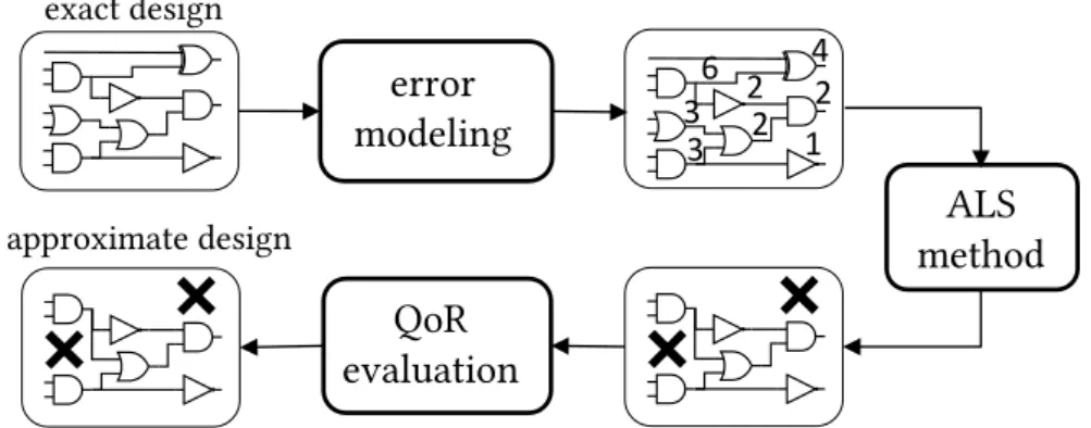
Figure 2.7 illustrates the Approximate Logic Synthesis flow that is followed in this thesis, which augments and improves the state of the art depicted in Figure 2.2. Here, the ALS core method is preceded by an error modeling phase.

Indeed, before applying a given approximation to an exact design, it is es-sential to estimate how much that transformation will impact on the final result. Therefore, an error modeling phase must be present, with the aim of annotating a circuit (or a Boolean) specification with a notion of error. This step provides an estimate – which can be more or less accurate, depending on the approach – of the potential error introduced by a given circuit simplification, which in turn

guidesALS methods in identifying the least error-prone transformation, or set of

transformations.

The importance of the presence of the error modeling phase is showcased in Figure 2.8, which illustrates the performance of an approximate circuit obtained by the GLP method [1] when guided by an accurate error modeling algorithm,

(32)

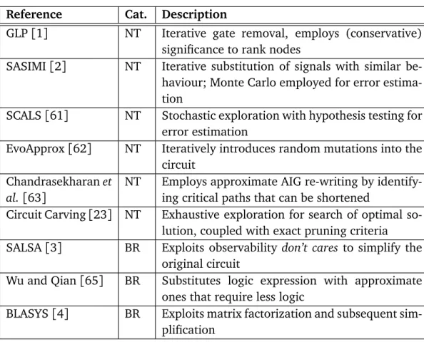
Table 2.1. Summary of the ALS works described, where NT stands for Netlist Transformation, and BR for Boolean Rewriting.

Reference Cat. Description

GLP[1] NT Iterative gate removal, employs (conservative) significance to rank nodes

SASIMI[2] NT Iterative substitution of signals with similar be-haviour; Monte Carlo employed for error estima-tion

SCALS[61] NT Stochastic exploration with hypothesis testing for error estimation

EvoApprox[62] NT Iteratively introduces random mutations into the circuit

Chandrasekharan et

al.[63]

NT Employs approximate AIG re-writing by identify-ing critical paths that can be shortened

Circuit Carving[23] NT Exhaustive exploration for search of optimal so-lution, coupled with exact pruning criteria SALSA[3] BR Exploits observability don’t cares to simplify the

original circuit

Wu and Qian[65] BR Substitutes logic expression with approximate ones that require less logic

BLASYS[4] BR Exploits matrix factorization and subsequent sim-plification

called PP-Mon[5], as opposed to its original implementation, which instead em-ploys a highly conservative error modeling strategy. Indeed, when guided by PP-Mon, GLP retrieves much smaller, faster and more efficient circuits for the same amount of tolerated error, as expressed by the Energy, Delay and Area Product (EDAP) on the y-axis.

Several ALS algorithms do not rely on the error modeling phase, such as Vasicek et al.[62], where a genetic programming technique is employed to ran-domly mutate the circuit and explore the search space without a priori notion of the induced error; however, the execution time and final QoR of these algorithms could highly benefit from an accurate error modeling phase.

Other works instead, such as Circuit Carving[23], compute a tight bound on maximum error in the first phase, and then the resulting simplified circuits do not need to undergo the QoR evaluation phase, as they are already guaranteed to not overtake such bound.

(33)

ALS

method

error

modeling

₁2 4 6 2 2 3 3

QoR

evaluation

approximate design exact design

Figure 2.7. A phase of error modeling can precede Approximate Logic Syn-thesis, with the aim of decorating a circuit (or a Boolean specification) with a notion of error, and hence guiding subsequent logic-simplification decisions. Then, the phase of QoR evaluation completes the process to verify whether output quality constraints are satisfied in the synthesised approximate circuit.

In the next section, the most commonly used error metrics for both error evaluation phases will be described, since their formal definition allows to un-derstand precisely how different algorithms of the state of the art approach error estimation. Next, the principal strategies for error modeling of the state of the art are described.

2.2.1 Error Metrics

When performing error profiling, a first step is to appropriately encode the bits at the output according to the intended representation (e.g., as signed or un-signed numbers). Hence, a difference d between an exact and approximate im-plemented Boolean functions ( f and ˜f, respectively) can be computed between two outputs for the same inputs:

d(f (x), ˜f(x)) = ||f (x) − ˜f(x)||

Then, an input-independent distance D must be derived from all values of d according to a metric. Alternative choices for such metric are influenced by sev-eral factors: the nature of the application in which the approximate hardware will be employed, its criticality, etc. For example, Ma et al. [69] and Venkatara-mani et al. [3] employ the Hamming Distance as a measure of d, defined as the number of bit flips in ˜f w.r.t. the original f .

(34)

Figure 2.8. Energy, delay and area (EDAP) reduction for different error con-straints in an 8-bit multiplier. For the same level of tolerated error, GLP guided by PP-Mon (red) obtains much smaller, faster and more efficient cir-cuits than its original implementation (green), which is guided by a simpler error modeling approach, called sum propagation.

defined. Referring again to the Hamming distance, one could be interested in the maximum or average Hamming distance over the inputs of f .

When, as done in[1,5,23,63], the focus is on controlling the Maximum Error (i.e., worst case distance) that occurs when a circuit is approximated, D is defined as:

max

x∈X(d(f (x), ˜f(x)))

expressing the maximum value of the difference between f and ˜f, being X the set of all possible circuit inputs and x a generic input.

Several Approximate Logic Synthesis techniques[1,2,4,61,65,70,71] moni-tor average case distance (Mean Absolute Error) induced on the output, instead of focusing on potential outliers, expressed as

Ex{d( f (x), ˜f(x))}

where the expectation is taken over the input data. If inputs are uniformly dis-tributed, the expression above becomes

(35)

1 |X |

X

x∈X

d(f (x), ˜f(x))

where |X | denotes the input set cardinality (i.e. the number of possible inputs). A related metric is the Mean Squared Error, in which distance terms are squared:

1 |X |

X

x∈X

(d(f (x), ˜f(x)))2

Distances are instead normalised by the (exact) output values size|| f || when considering the Average Relative Error Magnitude as an error metric:

1 |X | X x∈X d(f (x), ˜f(x)) || f (x)||

Moreover, it is often of interest to know how often errors occur in approxi-mate circuits, regardless of their magnitude. The Error Rate is a common metric that captures this phenomenon. For a generic circuit, given W = {x ∈ X |f (x) 6=

˜

f(x)} the set of inputs for which the approximate function computes an

erro-neous output, the Error rate is defined as: |W | |X |

It is of course possible for a given Approximate Logic Synthesis approach to consider more than one error metric. Indeed, in [3, 42, 60, 63, 64, 67, 72], both maximum error and average error are taken into account.

Some works introduce further metrics for error estimation that also consider the structure of the circuit being simplified, in addition to its functionality. No-tably, Zhang et al.[73] adopt the notion of Approximate Efficiency, defined as the ratio between the gain (in terms of Energy-Delay Product, E DP) deriving from the simplification of a node and the corresponding induced error: ∆EDP/D. The underlying assumption is that, if two nodes generate the same error in the final output when pruned from the original circuit, the one leading to higher benefits should be pruned first.

The works described in Chapter 3 and 4 mainly focus on maximum error estimation and control. However, Chapter 5 describes how these methods can be adapted to evaluate mean absolute error.

(36)

2.2.2 Methods for Error Modeling

Finally, there exist several possibilities to quantify the error metrics introduced above, each presenting some strengths and weaknesses:

Exact error evaluation. A precise computation of the error caused by a cir-cuit modification requires exhaustive evaluation for all possible input combina-tions. This number grows exponentially with the number of inputs, and hence such computation cannot scale to large circuits. SAT-solver based techniques were proposed [42] in order to help accelerating exhaustive evaluations; how-ever, exhaustiveness necessarily becomes intractable at some point, as the circuit size increases. Hence, the need arises for methods to efficiently calculate error estimates (in the case of average errors and error rates) and error bounds (for maximum errors).

Average error estimation. A widespread strategy to estimate average er-rors is to simulate a circuit for a subset of its inputs, randomly chosen through Monte Carlo selection [42], resulting in an unbiased statistical estimate of D. Nonetheless, even a Monte Carlo implementation can become computationally intractable for large circuits if carried out in a straightforward way, because it necessitates distinct evaluations, at each simplification step, for all candidate ap-proximate transformations. Su et al. [74] devise a technique that effectively lowers the computational effort entailed. The complexity of their algorithm, based on change propagation matrices that track the effects of an internal node to the primary outputs, is O (MOT ), where M is the size of the Monte Carlo in-put set, O the number of primary outin-put, and T is the size of the set of possible approximate transformations. A naïve Monte Carlo alternative has complexity O (M N T ), where N is the number of nodes in the circuit, which is usually much larger than the number of its primary outputs. However, T grows exponentially with the size of the circuit and, hence, for large circuits it may still be too heavy to derive accurate estimates of the error.

Bounding maximum errors. Monte Carlo-based approaches are not employ-able when maximum error thresholds must be provided, as they can not account for outliers. As described in Section 2.1.1, GLP by Schlachter et al.[1] introduces an algorithm to compute error guarantees, which assigns to each node in a circuit the sum of the significance of all its reachable outputs (where the significance of the output bit i is equal to 2i). This strategy is overly conservative, as it assumes that a node simplification can affect all reachable outputs simultaneously for at least one input combination (all ones becoming zeros, and vice-versa). In fact,

(37)

masking effects very often reduce the magnitude of perturbations caused by in-exact transformations, preventing all outputs to assume erroneous values at the same time.

Chapter 4 summarises the main characteristics of these methods, along with the presentation of an approach I devised that improves on the state of the art by concentrating the strengths of the three, and limiting their weaknesses.

The next chapter, instead, illustrates my work Circuit Carving, an ALS method that employs exact evaluation to guide structural netlist modification. The accu-racy on the induced error estimation combined with the exhaustive nature of the algorithm generate highly performant approximate circuits.

(38)

(39)

Circuit Carving: exhaustively exploring

approximations

3.1 Introduction

One of the first works of my PhD is an ALS algorithm called Circuit Carving (CC). This algorithm belongs to the category of structural netlist transformation, described in Chapter 2, but it presents a fundamental difference w.r.t. the other techniques in the state of the art: instead of employing heuristics for netlist mod-ification, it resorts to pruned exhaustive exploration in order to identify optimal solutions.

Having as input a generic combinatorial netlist, Circuit Carving identifies its largest sub-circuit that can be discarded, carved out of the original one, without violating a user-specified error constraint. As opposed to several works, which are based on iterative simplifications on the input circuit, the approximation problem is casted as a binary search tree exploration which exploits accurate knowledge of the circuit gate-level error distribution. While this formulation has exponential complexity, the scalability of the proposed method is improved by implementing search-pruning criteria that exploit the circuit topology in order to effectively reduce the exploration time.

The key contributions of this work can be summarised as follows:

• The description of a novel methodology, called Circuit Carving, for the de-sign of inexact digital circuits, which explores the search space of the exact circuit subsets.

• The introduction of pruning conditions that can effectively decrease the mentioned search space, and hence increase the framework scalability, by

(40)

disregarding search space regions that cannot contain candidate to optimal solutions.

• The employment of induction on identical blocks for error modeling of large circuits.

3.2 Problem formulation

The digital logic implementing a boolean function can be represented as a Direct Acyclic Graph (DAG)(N, E), where each node n_i∈ N represents a gate. An edge (ni, nj) ∈ E represents a connection from node ni to node nj, in that the output

of node ni is used by node nj.

Nodes are annotated with weights w_n_i, indicating the maximum difference visible at the circuit outputs, when setting the output of the node n_ito a constant value. The weight of an edge is equal to that of its destination node.

A cut (N_C, E_C), with N_C ⊂ N , EC ⊂ E, identifies a subgraph of the original

graph. An example of cut is shown by the dashed line in Figure 3.1a. The set

O(C) of the outgoing edges of a cut is defined as

O(C) := {(n_i, nj) ∈ EC | ni ∈ NC∧ nj /∈ NC}

If the outgoing edges of a cut are set to a constant value, 0 or 1, then the circuitry contained in the cut does not contribute to the circuit logic anymore, and the cut can therefore be suppressed. The resulting graph is, hence, a candidate inexact circuit.

The weight of a cut wC is defined as the sum of the weights of its outgoing

edges, and represents the maximal error introduced by removing from the exact circuit the gates corresponding to the nodes in C. In Figure 3.1a, cut C1 has

two outgoing edges, with weight 8 and 4 respectively, therefore wC1 = 12; the

methodologies that can be employed to derive such weights are explained later on, in Section 3.2.2; for now one shall assume these values known.

Circuit Carving (CC) aims at finding the largest cut(NC, EC) such that wC ≤ T ,

4

n

5

(a)

(b)

C

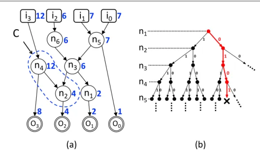
2 4 1 8 4 2 6 6 6 7 7 7 12 12

Figure 3.1. a) Example of a graph, and of a cut C within it. Labels besides

nodes represent their weight. The weight of cut C is 12 (sum of the differences

of its outgoing edges). b) The binary search path corresponding to cut C,

outlined in bold, red. Ifw_C > T, the search in this path stops and the algorithm

backtracks to the previous node.

3.2.1 Exploration Algorithm

To find such cut, the algorithm explores a search tree representing all subsets of graph(N, E). Each level of the exploration represents the inclusion (1-branch) or exclusion (0-branch) of node ni in a cut. Therefore, each cut(NC, EC) is

repre-sented by its corresponding path in the binary tree; Figure 3.1b shows the path corresponding to cut C of Figure 3.1a.

Since this formulation has worst-case exponential complexity, pruning crite-ria are necessary to reduce the search space and obtain a more scalable frame-work.

A cut is valid if its weight wC is not larger than T . Validity can be exploited

as a pruning criterion when node exploration is performed in reverse topological order, i.e., for all edges(u, v) ∈ E, v is explored before u (as done in Figure 3.1a). In this way, wC monotonically increases w.r.t. the exploration depth, because any

outgoing edge of a cut cannot be recovered. If at some level i the cut weight overcomes the pre-defined error threshold T , the inclusion of further nodes in the cut cannot result in a valid candidate, and the search can be stopped (as in Figure 3.1b, considering an error threshold T smaller than 12). This criterion is called validity and its effectiveness is quantified in Section 3.3.2.

(42)

closure, of a cut. Let us define the set of all parents of node n: P_n= {x | ∃(x, n) ∈

E_{}, and the set of all children Q}_n = {x | ∃(n, x) ∈ E}. A cut is closed if for all

nodes of the original graph it holds that: ¨

∀x ∈ Pn. x ∈ NC⇒ n ∈ NC

∀x ∈ Qn. x ∈ NC ⇒ n ∈ NC

2 O1 O2 O3

i

3

n

₃

Figure 3.2. a) Cut C2 is not closed, and cut C L(C2) represents its closure. b)

Exploration path for cutC₂. Sincen₃ _{∈ C L(C}₂), branch 0 from n₃ in Figure 3.2b is not explored.

The concept of closure is crucial for reducing the exploration space: only closed cuts must be considered as candidates, since non-closed cuts are, by defini-tion, sub-optimal. Therefore, the computation of closure C L(C) can be exploited to prune the search. In fact, whenever the algorithm is exploring a non-closed cut C, at level i, it computes its closure and verifies whether the next node ni+1

in the search belongs to C L(C). If it is so, it means that the current cut must be expanded to include node n_i₊₁, otherwise it could never represent a solution

(43)

to the problem. Hence, the 0-branch at node n_i₊₁ can be disregarded. An ex-ample of this criterion at work is shown in Figure 3.2b, where the 0-branches at nodes n3and n6are not explored. This pruning criterion is called closure, and its

effectiveness is also quantified in Section 3.3.2.

The third and last pruning criterion considers the number of gates included in the maximum cut found so far. If, at some level i, the sum of the nodes still to be considered plus the nodes already included in the cut is less than the size of the best candidate already found, the algorithm avoids exploring any further. This is the residual gain pruning criterion and its effectiveness is also quantified in Section 3.3.2.

The three aforementioned pruning criteria contribute to reducing the binary search tree exploration run-time by orders of magnitude, making the CC frame-work more scalable. However, for large circuits and large error values, the com-plexity of the exponential search may still result in unreasonable execution times. In these cases, an upper bound can be added on the number of recursive calls to limit the execution time and, of course, foregoing optimality. Results in Sec-tion 3.3.1 demonstrate that, even when the number of recursions is bounded, the CC framework is tangibly more performant when compared to the state of the art.

3.2.2 Error modeling

A preliminary step to the binary search tree exploration consists in identifying and assigning weights wn to all nodes n ∈ N . This process will be formally

defined and described in Chapter 4 , which presents different strategies for error modeling. In this Section, I present one of these strategies, whose strengths and weaknesses will be discussed in Chapter 4.

First, output nodes weights are set to their bit significance (as can be seen in Figure 3.1a: output o0 has weight 1, o1 has weight 2, o2 has weight 4 and so

on) and then weights are propagated upward. A conservative way to implement upward propagation is, for every gate having fanout more than one (such as n3

in Figure 3.1a), to compute the weight as the sum of the weights of its outgoing edges. This represents an upper bound for gate weight, since it would be impos-sible, when removing a gate, to produce a difference on the output larger than the sum of the bits reachable from that gate.

The exact values of weights for single gates, instead, can be obtained through exhaustive simulation. To do so, each gate is set to a constant value and the circuit deprived of that gate is simulated for all its input values; its output is then compared with the exact output, and w_n_i is set as the maximum obtained

(44)

abcin 2n+12n 000 001 010 011 100 101 110 111 00 01 01 10 01 10 10 11 (a) (b)

a

b

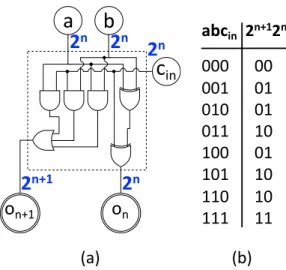
Figure 3.3. a) A full-adder labelled with its weights. b) Its truth table.

error. While node weight values are exact, our definition of cut weight w_C as the sum of its outgoing edges is still a conservative estimate. This is because, as in the example of Figure 3.3a, in many practical cases the removal of a cut cannot influence all its reachable outputs simultaneously.

Whenever the number of circuit inputs is too large to allow exhaustive gate-level simulation, two possible strategies can be adopted. The first one consists in running the simulations on a random subset of the circuit inputs instead of the whole set, but this would invalidate the exactness of the error modeling method. Otherwise, the graph topology can be exploited to infer, when possible, weight-propagation rules.

An example of the latter strategy application is the full-adder, depicted in Figure 3.3a. Consider the last full-adder of a ripple carry chain (output weights, therefore, 2n+1 and 2n); it can be observed from its truth table in Figure 3.3b that by setting to a constant value one bit in {a, b, cin}, while leaving the other

two unchanged, the maximum obtainable difference is 2n_{. Therefore, the three}

inputs of the full adder are labelled with the weight of the less significant output bit, i.e., 2n. Since this property holds for any of the previous full-adders of the carry chain, this weight can be propagated to derive the weights for a ripple carry adder of arbitrary length (Figure 3.4).

(45)

2n+1 ₂n ₂n-1 ₂n-2 ₂n-3 2n ₂n 2n 2n-1₂n-1 2n-1 2n-2₂n-2 2n-2 2n-3₂n-3

…

Figure 3.4. A 4-bit ripple carry adder with error modeling derived from weight-propagation.

3.3 Experimental evaluation

3.3.1 Performance of inexact circuits

To assess the performance of Circuit Carving, the approximate circuits obtained by it have been compared with those obtained by GLP [1], a greedy strategy belonging to the state of the art, and described in Chapter 2. In GLP, weights (called node significance in their work) are assigned through (conservative) sum propagation. Then, a greedy selection of nodes to be removed from the circuit is performed, and resulting netlists are iteratively simulated — for a subset of combinations of the inputs — to check for correctness. Nodes to be removed are chosen starting from those with lower weight. In practice, the GLP method corresponds to choosing a single path in the search space, without backtracking, as opposed to the entire exploration aware of the exact weights performed by Circuit Carving. This makes CC more computationally expensive, but also more effective, in terms of finding larger sub-circuits to be eliminated from the exact circuit.

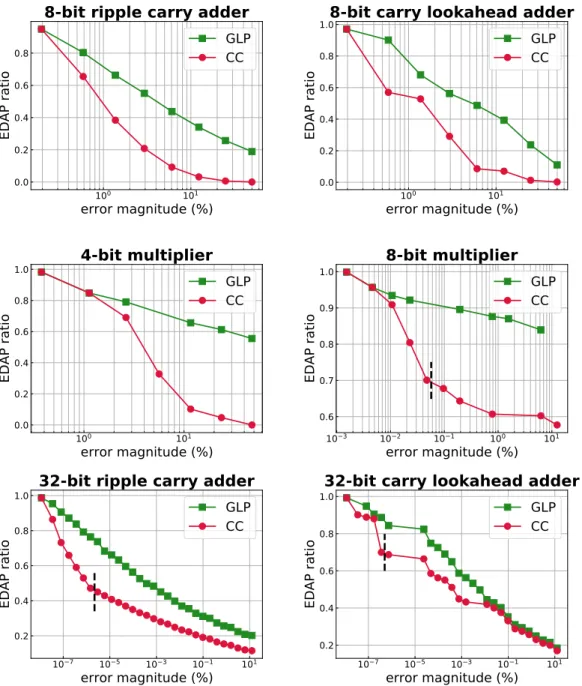
The trade-offs between performance and maximum tolerable error, for the inexact implementations designed with CC and GLP, can be observed in Figure 3.5. The figure of merit on the vertical axis is the Energy-Delay-Area Product (EDAP), normalized with respect to the corresponding exact circuit. The choice of evaluating EDAP, as opposed to only area savings, is to provide a more com-prehensive view on the result quality, as well as a fair comparison with the state of the art. The horizontal axis, error magnitude, indicates the maximum absolute error constraint, as a percentage of the maximum output of the circuit.

The figure showcases how the CC framework consistently achieves better re-sults across all benchmarks when compared to GLP, i.e.: it derives circuits with smaller EDAP for the same error constraint. As an example, CC reduces the EDAP

(46)

of an 8-bit multiplier by 40% when an error magnitude of 1% (i.e., an error of 1% of the maximum output) is tolerated, while GLP only leads to a∼10% EDAP reduction in that case.

Note that, for the smaller benchmarks processed in Figure 3.5, namely the 8-bit adders and the 4-bit multiplier, binary search tree exploration algorithm scaled for all possible error values. However, for the larger benchmarks, while exploration did terminate for small error values, it did not terminate — within a threshold of one hour of computation — for larger error values. The divide is shown by the vertical, dashed line in the graphs of the 32-bit adders and the 8-bit multiplier. For the points to the right of the vertical dashed line, where complete exploration was not performed, the best result achieved at the time of termination is reported. It can be seen that the CC methodology, even when stopped short of finishing the exploration, still finds larger subgraphs to be re-moved, resulting in approximate circuits with lower EDAP, when compared to GLP.

3.3.2 Effectiveness of Search Space Pruning

To quantify the effectiveness of the three search space pruning criteria (validity,

closure and residual gain), the exploration algorithm was run on the 8-bit

rip-ple carry adder benchmark, each time turning off some of the criteria, and the number of calls required to complete exploration in each case was plotted. Note that, since the criteria are exact, when they are turned off the solution found at the end of exploration is the same — but at the cost of more recursive calls being performed. Results are shown in Figure 3.6, which reports the number of recursive calls (capped at 109_{) required when different combinations of the three}

criteria were used.

The data shows that exploration does not terminate within 109calls when the

validitycondition is not considered. Compared to validity alone and for an error

magnitude of 5%, the combination of validity and closure results in a reduction of the search space of ∼10X, while applying validity and residual gain reduces it by ∼30X. When all three pruning criteria are used, a search space reduction of∼600X is achieved. For larger errors, the difference between curves increases even more, to several orders of magnitude, and finally, for extremely large er-ror values (which correspond to removing almost the whole circuit) exploration correctly converges extremely fast when the residual gain criterion is turned on. This work was published as a full paper at the DATE (Design, Automation and Test in Europe) conference in 2018[23].

CC

Figure 3.5. Energy-Delay-Area Product (EDAP) of the inexact circuits derived from our methodology and from the greedy approach of Schlachter et al. [1], varying the error constraint. EDAP values are normalized with respect to the exact implementations.

(48)

10-1 100 101 102

error magnitude (%)

101 103 105 107 109

# of c

alls

Eﬃciency of pruning criteria for 8-bit RCA

{2,3}

{1} {1,2} {1,3} {1,2,3}

Figure 3.6. Number of recursive calls in the binary search tree exploration algo-rithm, when different combinations of pruning criteria are applied: 1) validity, 2) closure and 3) residual gain.

(49)

A formal framework for error modeling

The previous chapters have introduced the idea that an accurate error model is fundamental for the performance of Approximate Logic Synthesis. Indeed, my latter research has focused on the definition and identification of algorithms for error modeling.

The strategies adopted so far to obtain an error model are of three different types: Monte Carlo sampling of the circuit inputs and simulation over the re-sulting input subset is a first possibility [2, 4, 74]. However, the accuracy of the weights obtained through this strategy relies entirely on the size of the sample and, most importantly, the obtained results do not guarantee any bound on the induced error.

Other works exhaustively evaluate such weights, either explicitly by fully sim-ulating the circuit, as in Circuit Carving [23], or implicitly by employing SAT-solvers [42]. While these strategies derive exact weights, they clearly present scalability problems when applied to large circuits, since their complexity is ex-ponential in the number of the circuit inputs.

Finally, conservative bounds can be adopted to estimate such weights by us-ing sum propagation, where node weights are assigned to the sum of all their children weights. However, such overly conservative weights have proven to provide poor guidance to the ALS method applied subsequently, as illustrated by my work [5], detailed later in this chapter. To sum up, each of these methods presents both strengths and weaknesses, outlined in Figure 4.1.

The approach proposed in this chapter introduces a powerful alternative to these methods. As in other state of the art algorithms, the circuit is represented as a Directed Acyclic Graph (DAG), and the final purpose is again to derive an error model which identifies bounds on the maximum error induced on the circuit output if a gate is removed from the circuit.