Carbon isotope ratios suggest no additional methane from boreal wetlands during the rapid Greenland Interstadial 21.2

HAL Id: hal-01805160

https://hal.archives-ouvertes.fr/hal-01805160

Submitted on 5 May 2021

HAL is a multi-disciplinary open access

archive for the deposit and dissemination of

sci-entific research documents, whether they are

pub-lished or not. The documents may come from

teaching and research institutions in France or

abroad, or from public or private research centers.

L’archive ouverte pluridisciplinaire HAL, est

destinée au dépôt et à la diffusion de documents

scientifiques de niveau recherche, publiés ou non,

émanant des établissements d’enseignement et de

recherche français ou étrangers, des laboratoires

publics ou privés.

Interstadial 21.2

Peter Sperlich, Hinrich Schaefer, Sara Mikaloff Fletcher, Myriam Guillevic,

Keith Lassey, Célia Sapart, Thomas Röckmann, Thomas Blunier

To cite this version:

Peter Sperlich, Hinrich Schaefer, Sara Mikaloff Fletcher, Myriam Guillevic, Keith Lassey, et al..

Car-bon isotope ratios suggest no additional methane from boreal wetlands during the rapid Greenland

Interstadial 21.2. Global Biogeochemical Cycles, American Geophysical Union, 2015, 29 (11), pp.1962

- 1976. �10.1002/2014GB005007�. �hal-01805160�

Carbon isotope ratios suggest no additional methane

from boreal wetlands during the rapid

Greenland Interstadial 21.2

Peter Sperlich1,2,3_{, Hinrich Schaefer}3_{, Sara E. Mikaloff Fletcher}3_{, Myriam Guillevic}1,4,5_,

Keith Lassey3,6_{, Célia J. Sapart}7,8_{, Thomas Röckmann}7_{, and Thomas Blunier}1

1_{Centre for Ice and Climate, University of Copenhagen, Copenhagen, Denmark,}2_{Max-Planck-Institute for}

Biogeochemistry, Jena, Germany,3_{National Institute of Water and Atmospheric Research, Wellington, New Zealand,} 4_{Laboratoire des Sciences du Climat et de l’Environnement, Gif sur Yvette, France,}5_{Now at Swiss Federal Institute of} Metrology, Bern-Wabern, Switzerland,6_{Lassey Research and Education Ltd, Lower Hutt, New Zealand,}7_{Institute for} Marine and Atmospheric Research Utrecht, Utrecht University, Utrecht, Netherlands,8_{Now at Laboratoire de Glaciologie,} Université Libre de Bruxelles, Brussels, Belgium

Abstract

4) to investigate the CH4mixing ratio anomaly during Greenland Interstadial (GI) 21.2 (85,000 years before present). This extraordinarily rapid event occurred within 150 years, comprising a CH4mixing ratio pulse of 150 ppb (∼25%). Our new measurements disclose a concomitant shift in𝛿13_C-CH

4of 1‰. Keeling plot analyses reveal the𝛿13C of the additional CH4source constituting the CH4anomaly as −56.8 ± 2.8‰, which we confirm by means of a previously published box model. We propose tropical wetlands as the most probable additional CH4source during GI-21.2 and present independent evidence that suggests that tropical wetlands in South America and Asia have played a key role. We find no evidence that boreal CH4sources, such as permafrost degradation, contributed significantly to the atmospheric CH4increase, despite the pronounced warming in the Northern Hemisphere during GI-21.2.

1. Introduction

Methane (CH4) is a strong greenhouse gas that is accumulating in Earth’s atmosphere due to human activity. Currently, CH4contributes 20% of the anthropogenic increase in radiative forcing since 1750 [e.g., Forster et al., 2007] and plays a significant role in recent and projected variations of global temperature, sea level, and sea ice extent [e.g., Meehl et al., 2007]. Reconstructions of atmospheric CH4mixing ratios (mixing ratios of all gases are indicated by [...] in the following) from ice core samples show distinct variations from decadal [e.g., Grachev

et al., 2007; Chappellaz et al., 2013; Mitchell et al., 2013] to orbital timescales [e.g., Loulergue et al., 2008]. Rapid

[CH₄] increases of the order of 150–300 ppb occurred over decades to centuries in association with Northern Hemispheric warm events [e.g., Brook et al., 1996; Grachev et al., 2007]. We use the most recent nomenclature after Rasmussen et al. [2014] and name the cold periods “Greenland Stadial” (GS) and the intermittent warm events “Greenland Interstadial” (GI).

High-resolution data sets show that some GI events were preceded by sharp precursor events of high ampli-tude, e.g., GI-21.2 [e.g., Grachev et al., 2007; Capron et al., 2010; Boch et al., 2011; Vallelonga et al., 2012;

Chappellaz et al., 2013; Deplazes et al., 2013]. The rapid GI-21.2 event about 85,000 years before 2000 A.D. (b2k)

comprised a [CH4] spike of ∼150 ppb that occurred within ∼150 years (Figure 1). This extraordinary event is marked by the highest [CH4] growth rate recorded in Greenland ice cores [Chappellaz et al., 2013]. Rapid [CH4] changes of this magnitude and timescale are of particular interest for studies on the biogeochemistry of CH4 and the sensitivity of CH4source fluxes to climate change.

Atmospheric chemistry models suggest that the [CH₄] variability during GI events was mostly driven by varia-tions in the sources of CH4rather than the sinks [Levine et al., 2012]. Atmospheric CH4sources have distinct iso-topic compositions in both𝛿13_{C and𝛿}2_{H that depend on the source processes and the CH}

4precursor material [e.g., Quay et al., 1999; Whiticar and Schaefer, 2007]. Observations of𝛿13_C-CH

4or𝛿2H-CH4can therefore con-strain CH4source flux reconstructions, which can then be interpreted in the context of climate variability [e.g., Ferretti et al., 2005; Schaefer et al., 2006; Sowers, 2006; Fischer et al., 2008; Bock et al., 2010; Sapart et al., 2012].

RESEARCH ARTICLE

10.1002/2014GB005007

Key Points:

• We present a𝛿13C-CH₄record of the rapid CH₄variation 85ka before present

• We apply Keeling plot analysis and validate the results against a box model

• We propose that tropical wetland emissions caused the observed CH₄anomaly

Correspondence to: P. Sperlich,

peter.sperlich@niwa.co.nz

Citation:

Sperlich, P., H. Schaefer, S. E. Mikaloff Fletcher, M. Guillevic, K. Lassey, C. J. Sapart, T. Röckmann, and T. Blunier (2015), Carbon isotope ratios sug-gest no additional methane from boreal wetlands during the rapid Greenland Interstadial 21.2, Global

Biogeochem. Cycles, 29, 1962–1976,

doi:10.1002/2014GB005007. Received 7 OCT 2014 Accepted 27 SEP 2015

Accepted article online 1 OCT 2015 Published online 30 NOV 2015

©2015. American Geophysical Union. All Rights Reserved.

Figure 1. [CH₄] spline fits for NEEM (blue) and NGRIP (black). Circles on the lines and bars at the bottom of the plot highlight the locations of the𝛿13_C-CH

4samples relative to [CH4].

Isotope records of CH₄suggest tropical and/or boreal wetland source flux variations as main drivers of the [CH₄] variability [e.g., Sowers, 2006; Fischer et al., 2008; Mischler et al., 2009; Bock et al., 2010; Möller et al., 2013]. Furthermore, isotopic evidence clearly demonstates that CH4hydrate destabilization was not the primary CH4source that caused the [CH4] variability during the last deglaciation [Sowers, 2006], GI-7 and GI-8 [Bock et al., 2010].

Most studies that analyzed the isotopic variability of CH4in ice core samples use mass balance calculations in box models [e.g., Ferretti et al., 2005; Schaefer et al., 2006; Sowers, 2006; Fischer et al., 2008; Mischler et al., 2009;

Bock et al., 2010; Sapart et al., 2012]. Here we investigate the change in𝛿13_C-CH

4that is associated with the [CH4] anomaly of GI-21.2 using Keeling plot analysis (KPA) [Keeling, 1958]. KPA is technically a two-component mixing model that provides the𝛿13_C-CH

4of an additional CH4source, which in our case is the source of the [CH₄] anomaly of GI-21.2. We present a Monte Carlo technique that considers both the analytical and data processing errors as well as a potential sampling bias in order to estimate the uncertainty of the KPA. Then, we compare the𝛿13_C-CH

4result from the KPA to the result from the forward stepping box model of Lassey et al. [2007] and show that the two methods agree well within the uncertainty of the KPA.

Recently, Möller et al. [2013] suggested that 𝛿13_C-CH

4 and [CH4] vary independently on millennial to glacial-interglacial timescales, which also questions the suitability of mass balance calculations for CH4source reconstructions on the timescales of our study period. We therefore test alternative scenarios where the

𝛿13_C-CH

4excursion of GI-21.2 is superimposed on a long-term𝛿13C-CH4trend that is controlled by [CO2]. We argue that KPA and mass balance calculations can be used in our study period when the effect of possible

𝛿13_C-CH

4background scenarios is carefully considered.

To our knowledge, this is the first time KPA is applied to studies of CH4in ice core samples. Therefore, we first review assumptions and necessary conditions for the use of KPA and then explain the processes that need to be considered in order to reconstruct the𝛿13_{C of an additional CH}

4source from ice core samples. Finally, we discuss and evaluate CH₄emission scenarios in the context of other, independent climate records.

2. Methods

2.1. Measurement Techniques

Our analytical technique for𝛿13_C-CH

4analysis is described in detail by Sperlich et al. [2013]. In short, cleaned ice core samples are melted in a vacuum system from which the liberated air sample is extracted. A helium carrier gas stream transports the sample through the analytical system to isolate CH₄and to combust it into CO₂before it is measured for𝛿13_{C on an isotope ratio mass spectrometer. Our𝛿}13_{C results are reported on the} Vienna Peedee Belemnite isotope scale, using the referencing technique described by Sperlich et al. [2012]. The analytical uncertainty of the𝛿13_C-CH

4measurements is 0.09‰. Our analytical method is free of kryp-ton artifacts which have recently been identified as a major problem in𝛿13_C-CH

4measurements [Schmitt et al., 2013].

Optical measurement techniques were recently applied to measure [CH4] in ice core samples [Stowasser et al., 2012] and provided a continuous record of unprecedented temporal resolution and precision from the NEEM ice core [Chappellaz et al., 2013]. This new method presents the [CH4] of GI-21.2 in unprecedented detail. Discrete [CH4] measurements from the NGRIP ice core show the anomaly of GI-21.2 in comparable magni-tude [Baumgartner et al., 2014]. We fitted two splines to the [CH4] records from Chappellaz et al. [2013] and Baumgartner et al. [2014] to calculate the mean [CH₄] of our𝛿13_C-CH

4samples (Figure 1). The spline of the NEEM data includes a 25 year smoothing filter, while replicate measurements of [CH₄] in the NGRIP record were averaged to avoid artifacts. The NEEM and the NGRIP spline fit show a slightly different timing for GI-21.2. However, timing offsets between the records can be corrected for because [CH₄] varies synchronously in the atmosphere [Blunier et al., 2007]. The higher temporal resolution of the NEEM [CH₄] record justifies to transfer the NGRIP [CH₄] data to the NEEM timescale for GI-21.2. Therefore, we used the NEEM spline in our box model calculations (section 2.6).

2.2. Ice Core Samples for𝜹13_C-CH

4Measurements

The rapid GI-21.2 event is recorded within only ∼1.5 m in the NEEM ice core [Chappellaz et al., 2013]. Because the number of available ice core samples from GI-21.2 and GS-22 is extremely limited (0.55 m ice per sample), we used samples from both the NEEM and NGRIP ice cores for𝛿13_C-CH

4analysis. We measured four samples of the stadial period preceding GI-21.2 (GI-22), when [CH4] was stable. We analyzed two samples of GI-21.2 and six younger samples of the strong [CH₄] variation of GI-21.1e (Figure 2). The age interval that is integrated within each of our𝛿13_C-CH

4samples from GS-22 and GI-21.2 is displayed in relation to the [CH4] history in Figure 1. Together, our two GI-21.2 samples integrate more than 50% of the event, including the [CH₄] peak and the highest rates of [CH₄] change.

2.3. Applied Corrections on𝜹13_C-CH

4Measurements All 𝛿13_C-CH

4 measurements are corrected for firn diffusion fractionation after Buizert et al. [2013]. This correction depends on the physical properties of the respective gas species, its relative growth rate, and a site-specific time-dependent factor, which is determined by the diffusive column height. The firn diffusion fractionation is generally smaller at Greenlandic than at central Antarctic sites. Our firn diffusion correction reaches maximum values of 0.34‰ during GI-21.2. This semiempirical method is published with a general, relative uncertainty of 30% for Greenland ice cores.

We also correct the𝛿13_C-CH

4and [CH4] data for the disequilibrium effect [Tans, 1997] that we determined with the box model of Lassey et al. [2007]. The disequilibrium effect for both𝛿13_C-CH

4and [CH4] is most pronounced for our GI-21.2 samples, where it accounts for up to 0.12‰ and 24 ppb, respectively. We discuss the relevance of this correction on our KPA results in section 3.1.

2.4. Assumptions for the Analysis of𝜹13_C-CH

4During Greenland Interstadial 21.2 Using Mass Balance Calculations

Because the limited amount of sample ice restricts the temporal data resolution, even our high-resolution record with an average resolution of one sample per 380 years includes a data gap of ∼1000 years, just before the onset of the GI-21.2 event. This requires an assumption as to the timing of the𝛿13_C-CH

4variation before the GI-21.2 event, which is critical for the analysis.

We can think of three different𝛿13_C-CH

4background scenarios: 1. The variation of𝛿13_C-CH

4is correlated with [CH4]; i.e., the𝛿13C-CH4background does not change before the onset of GI-21.2 (Figure 2c). This scenario is in agreement with most of the existing publications on

𝛿13_C-CH

4in ice core samples [e.g., Ferretti et al., 2005; Schaefer et al., 2006; Sowers, 2006; Fischer et al., 2008; Mischler et al., 2009; Bock et al., 2010; Sapart et al., 2012]. In particular, Melton et al. [2012] recently reported

a variation in𝛿13_C-CH

4in correspondence to a rapid change in [CH4]. In the following, we will refer to this as the [CH4]-correlated background scenario.

2. The𝛿13_C-CH

4is controlled by [CO2] on millennial to glacial timescales (Figure 2b) as recently published by Möller et al. [2013]. We will name this the [CO2]-correlated background scenario throughout this study. 3. A𝛿13_C-CH

4depletion that is continuous from the last measured pre-event value to the peak of GI-21.2 (Figure 2a).

Other evolutions of the𝛿13_C-CH

4 background cannot be ruled out but are highly speculative. We reject scenario 3 (as well as other𝛿13_C-CH

4background histories), because there is no mechanistic explanation for a𝛿13_C-CH

Figure 2. 𝛿13C-CH₄background scenarios: (leftyaxes) [CH₄], grey lines [Chappellaz et al., 2013]; (rightyaxes)𝛿13C-CH₄, filled symbols. Figures 2a–2c show the discussed scenarios of the𝛿13C-CH₄background during the sample gap between 85–86 ka b2k and the GI-21.2 event. (a) The𝛿13C-CH₄as direct (orange) line between measurements. (b) [CO₂] [Bereiter

et al., 2012],𝛿13C-CH4reconstruction based on the [CO2]-correlated background (red line) as determined by the

regression (red, dashed line); two arrows indicate the time lag between [CO2] and𝛿13C-CH4that averages to∼1270

years. (c)_𝛿13_C-CH

4reconstruction based on the [CH4]-correlated background scenario (red line). (d) The𝛿13C-CH4

measurements from NGRIP and NEEM ice cores. Note the good agreement between the 86 ka samples from both ice cores and the13_{C enrichment with decreasing [CH}

4] at the end of the GI-21.2 event. Green triangles (Figure 2d) indicate

points to match [CH₄] from the EPICA Dronning Maud Land (EDML) ice core [Schilt et al., 2010] and NEEM to transfer [CO₂] from the EDML gas age scale to GICC05_modelext [Blunier et al., 2007].

Also, the𝛿13_C-CH

4peak and decline of GI-21.2 indicate that the𝛿13C-CH4signal is indeed a positive excursion and not just part of a longer-term trend. Changes in [CH4] indicate variations in CH4emissions (assuming no or small sink variability). These necessarily incur changes in𝛿13_C-CH

4of the total source and consequently the atmosphere, except for the unlikely case that all sources change by the same relative amounts. Therefore, the coinciding excursions in [CH4] and𝛿13C-CH4can be analyzed for the underlying source changes [Ferretti et al., 2005; Schaefer et al., 2006; Sowers, 2006; Fischer et al., 2008; Mischler et al., 2009; Bock et al., 2010; Sapart et al., 2012]. The [CO2]-correlated𝛿13C-CH4variability [Möller et al., 2013] must also be taken into account. However, this can only explain a part of the GI-21.2𝛿13_C-CH

4excursion. A significant𝛿13C-CH4deviation linked to the [CH4] peak is evident even if superimposed on a longer-term, [CO2]-correlated trend in𝛿13C-CH4 (Figure 2b). Therefore, we hypothesize that scenarios 1 and 2 represent the outer bounds for the possible

evolution of the𝛿13_C-CH

4background, in agreement with previous publications. The𝛿13C-CH4excursion that is superimposed on the background trends can be analyzed with KPA and mass balance calculations because of its short duration of GI-21.2 and the likelihood of little variability in𝛿13_C-CH

4background. We present separate solutions for scenarios 1 and 2. Because there is no evidence to prefer either the [CH4]- or the [CO2]-correlated background scenario, we use the average of both analyses and their propagate uncertainty. Furthermore, we argue that our measurements and samples are appropriate to reconstruct the atmospheric variability of GI-21.2. Air is subject to mixing and diffusion processes in the firn column, before air is per-manently trapped in the ice [e.g., Buizert et al., 2012], which smoothes the recorded atmospheric signal. Ice core studies are therefore liable to underestimate atmospheric variability. However, previous studies showed excellent agreement between overlapping𝛿13_C-CH

4measurements in atmospheric, firn-air, and ice core sam-ples [Francey et al., 1999; Ferretti et al., 2005] (note that potential disagreements between multiple𝛿13_C-CH

4 firn-air records are largely based on analytical artifacts and laboratory offsets [Sapart et al., 2013] that may range in the order of 0.5‰ [Sapart et al., 2011]). The ice core samples from Ferretti et al. [2005] originated from a high-accumulation site where firn smoothing window is smaller than in central Greenland (≤20 years [Ferretti et al., 2005] versus≤80 years with mean of ∼25 years [Spahni et al., 2003]). Furthermore, the [CH4] growth rate was significantly larger during the time period studied by Ferretti et al. [2005] compared to that of GI-21.2 (5–17 ppb/yr [Etheridge et al., 1998] versus 2.5 ppb/yr [Chappellaz et al., 2013]), where a larger growth rate increases the impact of firn column effects. Therefore, we expect that firn smoothing has a neg-ligible effect on our record. Our two samples of the GI-21.2 event integrate about 50% of the [CH₄] variability (Figure 1), which might dampen the atmospheric signal. Because we average [CH₄] over the exact time period that is integrated in each𝛿13_C-CH

4sample for the KPA, we expect that the impact of the sample integration on the KPA result is not significant.

It is furthermore important to note that our𝛿13_C-CH

4samples integrate 40–70 years between sample top and bottom. For the KPA, we use [CH₄] and𝛿13_C-CH

4of identical ice cores and average [CH4] over the time period that is integrated in each𝛿13_C-CH

4sample. Because of this time integration, our analysis resolves variations as 40–70 year averages.

2.5. Keeling Plot Analysis

2.5.1. Keeling Plot Analysis for CH4Source Determination in Atmospheric Samples

For the KPA, the isotopic composition of a group of samples is plotted versus its inverse mixing ratio. The intercept of the linear regression with the y axis indicates the average isotopic signature of a trace gas source [Keeling, 1958]. This technique represents a two-component mixing model with background air and one addi-tional source of analyte gas as the only principal components [Pataki et al., 2003]. Pataki et al. [2003] express the global atmospheric budget as

c_a= c_b+ c_s (1)

where ca, cb, and csrepresent the CH4mixing ratios as measured in the atmosphere, the background atmo-sphere, and the term due to the additional source, respectively. While c_a and c_bare directly measured,

c_s can be calculated after equation (1), because we assume that the background is well defined by the measurements of c_b.

Referring to the isotopic composition of each term by𝛿13_{C, the mass balance calculation} 𝛿13_C

aca=𝛿13Cbcb+𝛿13Cscs (2) allows to calculate the𝛿13_C

sof the additional CH4source that accounts for csin the present-day atmosphere [e.g., Fisher et al., 2011].

2.5.2. Keeling Plot Analysis for CH₄Source Analysis in Ice Core Samples

Unlike for direct atmospheric measurements (e.g., in the vicinity of CH₄point sources), KPA on𝛿13_C-CH 4in ice core samples does not provide the isotopic composition of an additional CH4source directly, because two additional mechanisms have to be taken into account. There are the atmospheric disequilibrium effect [e.g.,

Tans, 1997] and the impact of the atmospheric sink fractionation (𝜀) on the 𝛿13_{C of the additional CH} 4source. Every ice core measurement needs to be corrected for the average disequilibrium effect per sample, which can be determined with a box model based on measured [CH4] and𝛿13C-CH4time series, resulting in𝛿13Ca−corr, 𝛿13_C

Figure 3. Keeling plots with uncertainties. (left) Keeling Plot with two measurements from GI-21.2 (blue circles) and

[CH₄]-correlated background as represented by four measurements from GS-22 (black circles). (right) Keeling Plot of [CO2]-correlated background, similar to Figure 3 (left) except that the two black circles indicate the two artificial data

points. Red lines represent the linear fit; grey and yellow shading illustrate the 95 and 99% confidence intervals of the linear fit as determined by the Monte Carlo analysis, respectively. Dotted lines indicate the least squares uncertainty; dashed lines indicate the uncertainty estimate of the “quasi” bootstrap.

fractionation of a similar magnitude as𝛿13_C

aand𝛿13Cb. By solving equation (2) for𝛿13Csand accounting for the disequilibrium effect correction and the sink weighted isotope fractionation (𝜀tot), we get

𝛿13_C s=

(𝛿13_C

a−corr× ca−corr−𝛿13Cb−corr× cb−corr) cs × ( 1 + 𝜀tot 1000 ) +𝜀_tot (3)

and are able to calculate the𝛿13_{C of the additional CH}

4source in ice core samples. 2.5.3. The Isotopic Fractionation of the Total CH4Sink in Keeling Plot Analysis

Literature values of𝜀totvary from −7.7‰ [Lassey et al., 2007] to −5.4‰ [Mischler et al., 2009], while it has been suggested to scale𝜀totto [CH4] on glacial-interglacial timescales [Schaefer and Whiticar, 2008]. The determina-tion of𝜀totdepends on the isotope fractionation of the respective CH4sinks and their relative contribution to the total sink fluxes. Note that both factors are likely to have varied on glacial-interglacial timescales and that the cumulative effect on𝜀_toton glacial timescales is not well understood [e.g., Schaefer and Whiticar, 2008;

Levine et al., 2012]. The weak correlation between [CH₄] and𝛿13_C-CH

4on millennial to glacial timescales [Möller et al., 2013] further suggests that the forcing of [CH4] on𝜀totis not controlling𝛿13C-CH4. We apply the𝜀totof −7.0‰ that Schaefer and Whiticar [2008] calculated for the preindustrial Holocene and discuss the effect of different𝜀totscenarios on our results in section 3.1.

2.5.4. Uncertainty Estimate of Least Squares Fit in Keeling Plot Analysis

A linear regression is used to calculate the slope and intercept of the KPA. This is often undertaken using a least squares fit, where the confidence interval of the fit is calculated based on the uncertainty of both slope and intercept, the degrees of freedom (n − 2), and the according quantiles of a Student’s t distribution at the chosen confidence level (Figure 3). We see two disadvantages of the least squares uncertainty in our case: 1. It requires homoscedasticity, whereas the residuals of our linear fit show a bimodal distribution of the

variance with clusters during the background period (GS-22) and during GI-21.2. The residuals of GI-21.2 data are larger by a factor of 2. Violating the precondition of homogenous variance of the residuals might therefore produce a data-specific bias, which we cannot investigate further because of the limited number of samples.

2. The least squares uncertainty neither considers the analytical uncertainty of 0.09‰ nor the uncertainty of the firn diffusion correction. The latter accounts for 0.11‰ in both GI-21.2 samples and for≤ 0.01‰ in all samples from GS-22 and GI-21.1e. The combined analytical uncertainty is thus clustered with higher uncertainties during GI-21.2, which is not reflected in the least squares scenario. We address these issues with a Monte Carlo estimate of the uncertainty.

2.5.5. Uncertainty Estimate of Keeling Plot Analysis Using Monte Carlo Technique

We designed a Monte Carlo simulation to determine 95 and 99% confidence intervals for least squares linear regressions based on the propagated uncertainties of each data point. In this approach, we randomly perturbed all data points independently, then performed a regression on the perturbed data, and repeated this process 10,000 times.

We calculated the perturbations as the sum of two perturbations, one based on a Gaussian distribution with a standard deviation equal to the measurement uncertainty (0.09‰) and one with a standard deviation equal to the data point specific uncertainty of the firn diffusion correction (0.01–0.11‰). These two perturbations were calculated independently, such that they might have an additive impact for some iterations and a cancel-ing effect for others. The 95 and 99% confidence intervals were then calculated as the 2.5–97.5 and 0.5–99.5 percentile values of the resulting regression curves. Because we have only two data points from GI-21.2, we constructed a quasi bootstrap method to account for errors from sampling bias. Here the same Monte Carlo routine used the background data of the four GI-22 samples, but it was assigned either one or the other data point of GI-21.2 twice, each time in combination with a new randomized uncertainty. This quasi bootstrap method calculates another two sets of 10,000 regressions for each case, that either of our two GI-21.2 samples represents the true value better than both values together. We show the 95 and 99% confidence intervals of the complete data set and furthermore the uppermost and lowermost 99% confidence interval boundaries of the quasi bootstrap in Figure 3. Note that the range between the latter two compares well to the uncertain-ties of the least squares method (section 2.5.4). We consider the Monte Carlo approach to be the more robust uncertainty estimate for several reasons: (1) It enables to calculate 95 and 99% of the linear fits that can all be seen as best scenarios within the uncertainty of our data. Therefore, it provides valuable, structural informa-tion of the uncertainty range. (2) It is free of assumpinforma-tions regarding the distribuinforma-tion of the residuals. (3) The quasi bootstrap method quantifies the sampling bias.

2.5.6. Determining the [CO2]-Correlated𝜹13C-CH4Background Scenario for Keeling Plot Analysis of GI-21.2

Möller et al. [2013] show the surprisingly strong correlation between𝛿13_C-CH

4and [CO2] during the last 160 ka and highlight periods when the correlation seems to break down, including the period after the onset of GI-21.1. The latter occurs during the 2300 year data gap in their record between 80.3 and 82.6 ka b2k Before the sample at 82.6 ka b2k, i.e., during our study period,𝛿13_C-CH

4and [CO2] seem to correlate [Möller et al., 2013, Figure 1]. However, the average temporal resolution of 1660 years in this part of the record from Möller

et al. [2013] complicates the precise timing of the correlation breakdown. Our data of this period are of higher

temporal resolution and show a correlation between the𝛿13_C-CH

4background and [CO2] during GS-22 and the early part of GI-21.1e, if we allow for an average time lag between [CO2] and𝛿13C-CH4of ∼1270 years (Figure 2b). Interestingly, this time lag is in agreement with Burckel et al. [2015], who found that changes in the Atlantic Meridional Overturning Circulation (AMOC) preceded precipitation changes in tropical South America during the last glacial period by 500–1700 years. This could provide an additional mechanistic clue to the correlation between [CO₂] and𝛿13_C-CH

4as interpreted by Möller et al. [2013], as the AMOC is related to changes in atmospheric [CO₂] [Bereiter et al., 2012] and the precipitation in South America to tropical CH₄ emissions, where the latter impact𝛿13_C-CH

4(Table 2). Note that independently of a precise determination of the time lag, the correlation between𝛿13_C-CH

4and [CO2] during the period just before and after GI-21.2 is evident. Therefore, the assumption of the [CO2]-correlated background scenario with monotonous𝛿13C-CH4 depletion around GI-21.2 is justified.

In order to determine the [CO2]-correlated𝛿13C-CH4background scenario, we use three of our measurements from GI-21.1e that are≤2000 years younger than GI-21.2. We fitted a regression through these three data points from GI-21.1e and the latest two measurements of GS-22 (red dashed line in Figure 2b). The resulting [CO2]-correlated background scenario for GI-21.2 and GS-22 is indicated by the thick red line in Figure 2b. Then, we calculated the𝛿13_C-CH

4in two points from just before and just after GI-21.2 based on the regression (black crosses in Figure 2b) and determined the corresponding [CH₄] data from Chappellaz et al. [2013] (Table 1). The two generated data pairs simulate a hypothetical background scenario for the case that the [CO₂]-correlated trend in𝛿13_C-CH

4represents the atmospheric𝛿13C-CH4variation around GI-21.2 more accurately than the [CH4]-correlated background (thick red line in Figure 2c). A KPA was then performed using the two artificial data points as background and our measured data from GI-21.2. This experiment highlights two important results: (1) GI-21.2 shows a significant𝛿13_C-CH

4event even when superimposed on a long-term𝛿13C-CH4 trend (Table 1). (2) Using both background scenarios for KPA leads to similar CH4source signatures that agree within the uncertainty estimate (Figure 3). In this study, the backgound assumption does not impact on our interpretation of the KPA result.

2.6. Configuration of a Box Model to Test Results From Keeling Plot Analysis

We configured the box model of Lassey et al. [2007] so that a base source and an additional source can be implemented in order to compare KPA and box model outputs. Specifically, the KPA assumes that atmosphere,

Table 1.𝛿13C-CH4and [CH4] Data Used for Keeling Plot Analysisa

Ice Core Age(ka b2k) _𝛿13_C-CH

4(‰) [CH4](ppb) NEEM 85.003 −47.83 635 NGRIP 85.036 −48.12 581 NGRIP 86.068 −46.85 472 NEEM 86.083 −46.84 444 NGRIP 86.964 −47.09 469 NEEM 87.301 −46.77 463 — 84.950 −47.56b ₅₅₃c — 85.150 −47.43b ₄₉₆c

a_{Columns 1–4 show sample site, mean gas age on the GICC05 time scale [Wolff}

et al., 2010].𝛿13C-CH₄after correction for firn diffusion fractionation, and mean [CH₄] per𝛿13C-CH₄sample, respectively.

b_{Artificial𝛿}13_C-CH

4values for [CO2]-correlated background (Figure 2b). c_[CH

4] values for [CO2]-correlated background from Chappellaz et al. [2013].

sources, and sink are in equilibrium, whereas the box model accounts for disequilibrium effects as discussed by

Tans [1997]. The CH₄source flux in the box model is set to reconstruct a smoothed spline fit (25 year smoothing window) of the NEEM [CH4] record from Chappellaz et al. [2013] (Figure 4a). The background source is config-ured to simulate the atmospheric [CH4] history during GS-22 by varying the source fluxes of background CH4 while a constant𝛿13_{C is assigned (Figure 4d). The𝛿}13_{C of background CH}

4was estimated as −53.6‰ by aver-aging the𝛿13_C-CH

4of our samples from GS-22 and correcting them for𝜀totof −7.0‰ (equation (3)). The onset of the GI-21.2 event occurs in the year 85,100 b2k in our [CH4] spline fit. The box model is configured to use a constant flux of the background source (fixed at the 85,100 b2k value) thereafter and to match the atmo-spheric [CH₄] history of GI-21.2 by varying the flux of the additional CH₄source (Figure 4e) with a𝛿13_C-CH

4 that can be varied. The𝛿13_C-CH

4value of the additional source is chosen so that the atmospheric𝛿13C-CH4 history is in best agreement with our two𝛿13_C-CH

4measurements from GI-21.2 (red circles in Figure 4e). We defined best agreement such that the difference to the modeled𝛿13_C-CH

4history is identical for both of our 𝛿13_C-CH

4samples. The box model solves for the𝛿13C of the additional CH4during GI-21.2, which we compare to the𝛿13_C-CH

4result of the KPA. We also apply the𝛿13C-CH4background of the [CO2]-correlated scenario in a box model run to compare the results to the KPA.

In addition, the box model is used to estimate the disequilibrium effect that results from changes in CH₄source fluxes and the𝛿13_{C of CH}

4sources [Tans, 1997]. The impact of the disequilibrium effect on𝛿13C scales with 𝜀tot, where a stronger sink fractionation causes a stronger disequilibrium. The disequilibrium effect variation during GS-22 and GI-21.2 is shown in Figures 4b and 4c. It is used to correct both the𝛿13_{C and the mean [CH}

4] of our𝛿13_C-CH

4samples for the KPA (equation (3)) and has a small impact on our KPA result.

3. Results

3.1. Results From Keeling Plot Analysis

Our 𝛿13_C-CH

4 measurements, the corresponding [CH4] data, and the two pairs of artificial data for the [CO2]-correlated background scenario are shown in Table 1. The KPA with [CH4]-correlated𝛿13C-CH4 back-ground intersects the y axis at −57.4‰ (Figure 3, left). We derive a conservative uncertainty estimate of ±2‰ from the 99% interval of the quasi bootstrap technique (section 2.5.5). The KPA for the [CO₂]-correlated back-ground scenario intersects the y axis at −56.1±2‰ (Figure 3, right). The difference between the two KPA results is 1.3‰, which is well within the uncertainty. The good agreement between KPA using both back-ground scenarios suggests that the assumption regarding the backback-ground variation of𝛿13_C-CH

4during GS-22 is not critical for our interpretation of the results.

Applying the𝜀totof −5.4‰ from Mischler et al. [2009] to our analysis would shift the KPA results by 1.5‰ toward more enriched𝛿13_{C values. Scaling𝜀}

totto [CH4] due to changes in the soil sink flux as suggested by Schaefer and Whiticar [2008] would result in an𝜀_totfor GS-22 and GI-21.2 of −5.9‰ and −6.5‰, respectively, if all other sink fluxes and𝜀 values remained constant. This would increase the difference in 𝛿13_{C between the}

Figure 4. Box model data. (a) The [CH₄] input data [Chappellaz et al., 2013] with GI-21.2 highlighted in green. (b and c) The calculated disequilibrium effect for [CH₄] and𝛿13C-CH₄, respectively. (d and e) The calculated CH₄fluxes of the background source and the additional source during GI-21.2, respectively. (f ) The𝛿13C-CH₄output from the box model in comparison to our𝛿13C-CH₄measurements before (red circles) and after (grey circles) the disequilibrium correction.

𝜀tot-corrected GS-22 and GI-21.2 data by 0.6‰ and shift the𝛿13C of the total sources toward more enriched values. The scaled𝜀totscenario would deplete the KPA results by 1.3‰. Note that none of these𝜀totscenarios would change our KPA results beyond the uncertainty envelope of ±2‰ and would therefore not change our interpretation of the results.

Applying the disequilibrium correction (equation (3)) shifts the KPA results by 0.4‰ toward stronger𝛿13_C enrichment, which is a small effect compared to the KPA uncertainty of ±2‰.

3.2. Comparing the Results From Keeling Plot Analysis and Box Model

The box model resulted in a𝛿13_{C of the additional source that is 0.6‰ more depleted in𝛿}13_{C than the KPA} result of the [CH₄]-correlated𝛿13_C-CH

4background. For the [CO2]-correlated background scenario, the box model result is 0.4‰ more enriched in𝛿13_{C. The difference between KPA and box model results is of different} sign for both scenarios but well within the ±2‰ uncertainty of the KPA. The disagreement between KPA and box model is partly due to the different methods used to determine the mathematical solution. While the KPA result is determined by a least squares fit that considers all data points from GI-21.2 and GS-22, the box model result depends on an equal mismatch between the modeled𝛿13_C-CH

Table 2. Average𝛿13_{C Isotope Ratios of Categorized CH} 4Sourcesa Source 𝛿13C-CH₄(‰) Tropical wetlands −58b Boreal wetlands −63b CH₄hydrates −62.5b Aerobic C3 −58c Aerobic C4 −50c Termites −70d Geological −40e Biomass burning −25d Thermokarst lakes −70f

a_{The data represent average values with an uncertainty of}

2–5‰ [e.g., Quay et al., 1999] or even larger for CH4 hydrates

[e.g., Kvenvolden, 1995].

b_{From Whiticar and Schaefer [2007] for glacial periods.} c_{From Keppler et al. [2006].}

d_{From Mikaloff Fletcher et al. [2004].} e_{From Denman et al. [2007].} f_{From Walter et al. [2008].}

points. Furthermore, the [CH4] at the begin-ning of the GI-21.2 event is ∼20 ppb higher than the mean [CH4] of the background samples from GS-22. To compensate this larger proportion of 𝛿13_C-enriched back-ground CH₄in the box model, the𝛿13_{C of the} additional CH₄has to be more depleted. Note that this is not the case for the box model test with the [CO₂]-correlated background, which may explain the change of sign in the difference.

3.3. Averaging the Keeling Plot Analyses Results of Both Background Assumptions for Interpretation

For our interpretation, we average the KPA results using the [CH4]- and the [CO2]-correlated background scenarios to −56.8±2.8‰. The averaged result consid-ers both background scenarios as equally possible solutions within the propagated uncertainty range.

4. Discussion

4.1. Applicability of Keeling Plot Analysis to Study the Variation of𝜹13_C-CH

4in Ice Core Samples We use KPA for the analyis of𝛿13_C-CH

4in ice core samples and derive results that agree with a forward stepping box model within the uncertainty of the KPA. For most accurate results, the KPA requires the disequi-librium correction, which can be calculated using a suitable box model in addition to the KPA. However, the disequilibrium correction did not change our KPA results significantly. The disequilibrium effect could be rel-atively small in our analysis because each of our𝛿13_C-CH

4samples averages a large part of the GI-21.2 event; hence, extreme values of the disequilibrium effect are smoothed out. This could be different for the analy-sis of samples with a similar but longer-lasting [CH4] gradient or samples that integrate a shorter period of time. However, the [CH₄] growth rate during GI.21.2 is to date the highest observed for natural [CH₄] variabil-ity [Chappellaz et al., 2013]. Therefore, it seems unlikely that the disequilibrium effect will have a significant impact on a KPA that is performed on other ice core samples during other periods of time.

Besides the fact that KPA can serve as a fast approach for𝛿13_C-CH

4analysis, it has the advantage over a box model that it is independent of a gas age scale, as KPA only requires the combination of CH4and𝛿13C-CH4 data. This avoids uncertainties from dating issues that may arise when data sets from more than one ice core are merged for analysis.

4.2. CH4Source Identification From Keeling Plot Analysis Result

Our averaged KPA result of −56.8±2.8‰ is in best agreement with the𝛿13_{C that Whiticar and Schaefer [2007]} reconstructed for CH₄emissions from tropical wetlands during the glacial period (Table 2). Note that aerobic formation of CH₄in C3 plants is a theoretical solution; however, the process and its relevance are not well understood and can therefore not be discussed in the context of rapid climate changes.

Our preferred solution is that tropical wetland emissions were the most important contributors to the [CH4] anomaly of GI-21.2. This result is supported by Baumgartner et al. [2014], who found that high growth rates, as reported for GI-21.2 [Chappellaz et al., 2013], are associated with an Intertropical Convergence Zone (ITCZ) position that enhances CH₄emissions from tropical Asia. Another method to constrain the spatial distribution of CH₄emissions is the relative Inter-Polar Difference (rIPD) of CH₄[e.g., Chappellaz et al., 1997; Brook et al., 2000; Baumgartner et al., 2014], which is strongly influenced by solar insolation [e.g., Baumgartner et al., 2014]. Because no rIPD reconstruction exists specifically for GI-21.2, we assume that the rIPD of the directly following GI-21.1e is indicative for GI-21.2. This assumption is justified by a maximum insolation gradient between 30∘N and 60∘N during both GI-21.1e and GI-21.2, with higher insolation in the lower latitudes [Laskar et al., 2004].

The rIPD during GI-21.1e appears to be of medium amplitude with ∼7.5%, which indicates the dominance of tropical Northern Hemisphere CH4sources [Baumgartner et al., 2014].

Predominant contributions from13_{C-depleted CH}

4sources like boreal wetlands would have to be compen-sated by emissions from13_{C-enriched CH}

4sources (such as pyrogenic CH4) to match the isotope budget. Such a scenario cannot be ruled out by our data but is not consistent with the geographic constraints for the addi-tional CH4emissions described above. The KPA precludes either biomass burning or termites as main CH4 source for the GI-21.2 anomaly (Table 2). Interestingly, an outstanding CH4emission pulse from geological mantle sources can also be ruled out, as this CH₄source is significantly more enriched in13_{C [e.g., Etiope and} Lollar, 2013]. The wide𝛿13_{C range of marine hydrate-bound CH}

4between −57 and −73‰ [e.g., Kvenvolden, 1995] with the additional potential for postemission enrichment by microbial oxidation in the water column [e.g., Whiticar and Faber, 1986] does not rule out CH4hydrate destabilization as the cause of the [CH4] anomaly during GI-21.2.

To investigate this further, we calculate a Rayleigh distillation as described by Schaefer et al. [2006] and find a theoretical CH4hydrate emission scenario in which ∼47% of released CH4is oxidized in sediment and water column while the remaining ∼53% reach the atmosphere in agreement with our KPA result. However, this partitioning between CH₄oxidation and release to the atmosphere is in strong disagreement with the obser-vations of Yvon-Lewis et al. [2011], who show that only 0.01% of the CH4that was released during the “Deep Water Horizon” spill arrived in the atmosphere. Based on𝛿2_H-CH

4data, Sowers [2006] and Bock et al. [2010] proved that marine hydrate destabilization did not cause the [CH4] increase during the last deglaciation and of GI-7 and GI-8, respectively. For the above mentioned reasons, we assume that it is unlikely that CH₄released from marine hydrates has caused the [CH₄] variability during GI-21.2.

In general, it is important to remember that the complex biogeochemistry of natural CH4sources leads to wide𝛿13_{C ranges within each source category, thereby limiting the constraining power of𝛿}13_C-CH

4 recon-structions. In the following, we compare our hypothesis that mostly tropical CH₄sources have caused the [CH4] anomaly during GI-21.2 to independent evidence.

5. Comparison to Independent Climate Records

The strong temperature variability as recorded in Greenland ice cores during the last glacial (e.g., NGRIP

community members [2004] and Figure 5c) is associated with changes in both atmospheric and ocean

cir-culation [e.g., Chiang and Friedman, 2012]. Variations in both are of hemispheric extent and are related to the location of the ITCZ [Chiang and Friedman, 2012; Burckel et al., 2015]. The ITCZ location is critical for the regulation of monsoon system intensities by controlling the meridional transport of heat and moisture [Chiang and Friedman, 2012; Burckel et al., 2015], which are the main controlling measures of CH₄emissions [Guo et al., 2012]. Thus, the ITCZ location determines the meridional distribution of CH4source regions and thereby the partitioning of CH4emissions from the Northern and Southern Hemispheres [e.g., Guo et al., 2012; Baumgartner et al., 2014]. In the following, we discuss the variation of climate proxies in a geographical context

in order to test our hypothesis that the CH4excursion during GI-21.2 was predominantly caused by increased CH₄emissions from tropical wetlands.

5.1. South American Monsoon Systems During Greenland Interstadial 21.2

Wang et al. [2004], Cruz et al. [2005], and Deplazes et al. [2013] reconstruct large-scale precipitation variations

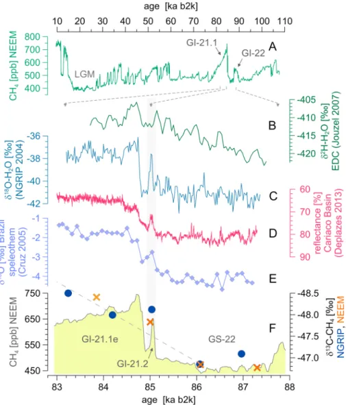
in South American rainforest systems: During GS-22, the Atlantic rainforest section of southern South America experienced a wet interval [Wang et al., 2004; Cruz et al., 2005] (Figure 5e), thereby enhancing CH4emissions from this region in the Southern Hemisphere. At the same time, marine sediment reflectivity records from the Cariaco Basin indicate that the climate in the much larger Amazonian rainforest system was in a dryer phase [Deplazes et al., 2013] (Figure 5d), which can be expected to reduce CH₄emissions from the Amazonian region. After GS-22, the large-scale precipitation pattern over South America changed significantly, most likely driven by solar insolation and changes in ocean circulation [Wang et al., 2004; Burckel et al., 2015]. The transition between the two states is resolved in both the Caricao Basin sediments [Deplazes et al., 2013] and the sub-tropical speleothem records from south Brazil [Cruz et al., 2005], where both records indicate a wetter climate period in the Amazonian rainforest systems during GI-21.2 (Figures 5d and 5e). Deplazes et al. [2013] propose a strong precipitation increase in the Amazonian rainforest that coincided with the temperature and [CH4] anomaly of GI-21.2, thereby linking Greenlandic and South American climate. The ITCZ controlled precipita-tion pattern in South America [Wang et al., 2004; Cruz et al., 2005; Deplazes et al., 2013] may result in a change

Figure 5.𝛿13C-CH₄in comparison to independent climate data. (a) [CH₄] during last glacial [Chappellaz et al., 2013] on the topxaxis. Figures 5b–5f refer to the bottomxaxis. The grey bar highlights the GI-21.2 event. (b) Antarctic and (c) Greenlandic water isotope ratios (Jouzel et al. [2007] and NGRIP [2004], respectively). (d) Reflectivity record of Cariaco Basin [Deplazes et al., 2013] and (e)𝛿18O from south Brazilian speleothems [Cruz et al., 2005]. (f ) Left axis [CH4] and right

axis (inverted)𝛿13C-CH4from NGRIP (circles) and NEEM (crosses). All data are shown on the GICC05_modelext timescale

[Wolff et al., 2010]._𝛿18_{O Figure 5e is adjusted by +0.55ka to align GI-21.2, which is in line with Cruz et al. [2005].}

of the dominant South American CH4source regions from the smaller Atlantic to the much larger Amazonian region between GS-22 and GI-21.2, possibly triggering CH4fluxes from Amazonian wetland sources to cause the [CH₄] anomaly of GI-21.2.

5.2. Asian Monsoon Systems During Greenland Interstadial 21.2

Pausata et al. [2011], Deplazes et al. [2013], and Mohtadi et al. [2014] propose a teleconnection pattern where

North Atlantic cold periods coincided with dryer conditions in the tropical Indian monsoon realm, mediated by changes in atmospheric circulation. Speleothem records of Wang et al. [2001, 2008] provide geological evi-dence that link Greenland climate with the transport of heat and moisture in the distant East Asian monsoon region. A further geological argument for a tight coupling between Greenland temperature and the Asian monsoon system is suggested by Ruth et al. [2007], according to which the lower dust concentration observed in Greenland ice cores during GI-21.2 [e.g., Rasmussen et al., 2014] indicates an intensification of the Asian monsoon system. The above mentioned studies suggest warmer and wetter climate in the Asian monsoon region during GI-21.2, where both factors potentially raise tropical wetland CH4emissions [e.g., Brook et al., 1996; Guo et al., 2012].

5.3. Potential for Boreal and Pyrogenic CH₄Emissions During Greenland Interstadial 21.2

Guo et al. [2012] describe that enhanced monsoon system strength (sections 5.1 and 5.2) increases the

merid-ional transport of heat and moisture into the extratropics, thereby strengthening boreal CH4emissions. Also, high Northern Hemisphere summer insolation [Laskar et al., 2004] and the relatively warm polar temperatures [EPICA, 2006] during GI-21.2 had the potential to enhance CH4emissions from boreal wetlands [e.g., Brook et al., 1996]. However, the CH4of boreal wetland sources is relatively depleted in13C and ranges around −63‰ (Table 2). Moreover, McCalley et al. [2014] report a further, systematic𝛿13_{C depletion of CH}

4emissions from newly degrading permafrost soils, which we cannot rule out during the rapid Northern Hemisphere warming of GI-21.2 [NGRIP, 2004]. Therefore, our result of −56.8±2.8‰ precludes boreal wetland emissions as the pre-dominant CH₄source causing the [CH₄] anomaly of GI-21.2 (Table 2). Increased boreal CH₄emissions would have to be compensated by13_{C-enriched pyrogenic CH}

4emissions (−25‰) during the period integrated per 𝛿13_C-CH

4sample to match our reconstructed𝛿13C-CH4. Daniau et al. [2007] analyzed charcoal records and found increased wildfire intensity in Europe during interstadial periods of the last glacial period, which would be consistent with this scenario.

On the contrary, charcoal records from lower latitudes suggest minimum wildfire intensities during our study period [e.g., Bird and Cali, 1998; Wang et al., 2005; Kershaw et al., 2007]. Given that Thonicke et al. [2005] report a consistent latitudinal pattern of highest charcoal counts and pyrogenic CH4emissions in the lower latitudes and found that this pattern was more pronounced during the LGM, the lack of evidence for increased tropi-cal burning during our study period suggests that global pyrogenic CH4formation was small. Consequently, CH4emissions from boreal wetland sources must have been small as well to meet the𝛿13C-CH4constraint. This finding strengthens our interpretation that tropical wetlands were the most important CH₄sources that caused the [CH₄] anomaly of GI-21.2.

6. Conclusions

We present an approach to use Keeling plot analysis to investigate the variability of CH4sources in ice core samples, based on𝛿13_C-CH

4and [CH4] measurements during GI-21.2. Our Keeling plot analysis includes a correction for the disequilibrium effect, based on information from a time stepping box model. The result of the Keeling plot analysis agrees with the box model results within 0.6‰, which is well within the uncertainty of the Keeling plot analysis (±2‰) for either of the background scenarios.

The average𝛿13_C-CH

4of the source causing the rapid [CH4] variability is best matched by enhanced CH4 emis-sions from tropical wetlands. Our conclusion is supported by a range of independent climate records, which suggest wetter and warmer climate in tropical Amazonian and Asian CH4source ecosystems. Increases in both boreal wetlands and biomass burning were only possible if their relative contributions produced the𝛿13_{C of} CH₄sources suggested by the KPA. Because charcoal records from lower latitudes suggest that the wildfire intensity during our study period was low, a strong response of boreal CH₄sources to the rapid GI-21.2 event seems unlikely. The hypothesis that boreal CH4sources showed a low sensitivity to the short but rapid tem-perature increase of GI-21.2 [e.g., NGRIP, 2004; Capron et al., 2010; Boch et al., 2011] is an interesting finding in the light of global warming and the associated potential for CH4emissions from boreal sources such as per-mafrost (note that GI-21.2 is not a complete analogue for present-day climate conditions). Further research including climate-vegetation modeling and atmospheric observations at highest spatiotemporal resolution is needed to provide reliable scenarios of vegetation dynamics and related changes in isotope ratios of CH4 emissions in order to fully exploit the information provided by CH₄isotope records from ice cores.

References

Baumgartner, M., et al. (2014), NGRIP CH4concentration from 120 to 10 kyr before present and its relation to a𝛿15N temperature

reconstruction from the same ice core, Clim. Past, 10, 903–920.

Bereiter, B., D. Lüthi, M. Siegrist, S. Schüpbach, T. F. Stocker, and H. Fischer (2012), Mode change of millennial CO₂variability during the last glacial cycle associated with a bipolar marine carbon seesaw, Proc. Natl. Acad. Sci. U.S.A., 109(25), 9755–9760.

Bird, M. I., and J. A. Cali (1998), A million-year record of fire in sub-Saharan Africa, Nature, 394, 767–769.

Blunier, T., R. Spahni, J. M. Barnola, J. Chappellaz, L. Loulergue, and J. Schwander (2007), Synchronization of ice core records via atmospheric gases, Clim. Past, 3(2), 325–330.

Boch, R., H. Cheng, C. Spotl, R. L. Edwards, X. Wang, and P. Hauselmann (2011), NALPS: A precisely dated European climate record 120–60 ka, Clim. Past, 7(4), 1247–1259.

Bock, M., J. Schmitt, L. Möller, R. Spahni, T. Blunier, and H. Fischer (2010), Hydrogen isotopes preclude marine hydrate CH₄emissions at the onset of Dansgaard-Oeschger events, Science, 328(5986), 1686–1689.

Acknowledgments

We thank everyone involved in logistics, field work, and ice core processing and analysis in the laboratories and during the field cam-paigns at NEEM and NGRIP. We would also like to thank Willi A. Brand and Martin Heimann for insightful discus-sions on CH₄isotopes and KPA as well as the two anonymous review-ers and the Editor for their valuable comments. We acknowledge the availability of data we used for our analysis and Figures. The [CH₄] (NEEM) reconstructions were provided by Thomas Blunier (blunier@nbi.ku.dk). All other data were obtained from the following sources:𝛿18O (NGRIP): World Data Center for Paleoclimatology and NOAA Paleoclimatology Program (ftp://ftp.ncdc.noaa.gov/pub/data/ paleo/icecore/greenland/summit/ ngrip/isotopes/ngrip-d18o-50yr.txt);

𝛿2_{H (EDC): NOAA national climatic}

data center (http://www.ncdc.noaa. gov/paleo/pubs/jouzel2007/ jouzel2007.html); CO₂(EDML): NOAA national climatic data center (ftp://ftp.ncdc.noaa.gov/pub/data/ paleo/icecore/antarctica/edml-talos2012co2.txt); CH₄(EDML): World Data Center for Paleoclimatology and NOAA Paleoclimatology Program (ftp://ftp.ncdc.noaa.gov/pub/data/ paleo/icecore/antarctica/maud/ edml-ch4-140k.txt); Marine sediment reflectance (Cariaco Basin): Pangaea, (http://doi.pangaea.de/10.1594/ PANGAEA.815882); and𝛿18O (speleothems): World Data Center for Paleoclimatology and NOAA Paleoclimatology Program (ftp://ftp.ncdc.noaa.gov/pub/data/ paleo/speleothem/southamerica/ brazil/botuvera2005.txt). This work is a contribution to the NGRIP ice core project, which is directed and organized by the Ice and Climate Research Group at the Niels Bohr Institute, University of Copenhagen. It is being supported by funding agencies in Denmark (SNF), Belgium (FNRS-CFB), France (IPEV, INSU/CNRS and ANR NEEM), Germany (AWI), Iceland (RannIs), Japan (MEXT), Sweden (SPRS), Switzerland (SNF), and the U.S. (NSF). NEEM is directed and organized by the Centre of Ice and Climate at the Niels Bohr Institute and U.S. NSF, Office of Polar Programs. It is supported by funding agencies and institutions in Belgium (FNRS-CFB and FWO), Canada (NRCan/GSC), China (CAS), Denmark (FI), France (IPEV, CNRS/INSU, CEA, and ANR), Germany (AWI), Iceland (RannIs), Japan (NIPR), South Korea (KOPRI), the Netherlands (NWO/ALW), Sweden (VR), Switzerland (SNF), the United Kingdom (NERC), and the U.S. (U.S. NSF, Office of Polar Programs). The research leading to these results has received funding from the European

Brook, E. J., T. Sowers, and J. Orchardo (1996), Rapid variations in atmospheric methane concentration during the past 110,000 years,

Science, 273(5278), 1087–1091.

Brook, E. J., S. Harder, J. Severinghaus, E. J. Steig, and C. M. Sucher (2000), On the origin and timing of rapid changes in atmospheric methane during the last glacial period, Global Biogeochem. Cycles, 14(2), 559–572.

Buizert, C., et al. (2012), Gas transport in firn: Multiple-tracer characterisation and model intercomparison for NEEM, Northern Greenland,

Atmos. Chem. Phys., 12(9), 4259–4277.

Buizert, C., T. Sowers, and T. Blunier (2013), Assessment of diffusive isotopic fractionation in polar firn, and application to ice core trace gas records, Earth Planet. Sci. Lett., 361, 110–119.

Burckel, P., C. Waelbroeck, J. M. Gherardi, S. Pichat, H. Arz, J. Lippold, T. Dokken, and F. Thil (2015), Atlantic Ocean circulation changes preceded millennial tropical South America rainfall events during the last glacial, Geophys. Res. Lett., 42, 411–418.

Capron, E., et al. (2010), Millennial and sub-millennial scale climatic variations recorded in polar ice cores over the last glacial period,

Clim. Past, 6(3), 345–365.

Chappellaz, J., T. Blunier, S. Kints, A. Dällenbach, J. M. Barnola, J. Schwander, D. Raynaud, and B. Stauffer (1997), Changes in the atmospheric CH₄gradient between Greenland and Antarctica during the Holocene, J. Geophys. Res. Atmos., 102(D13), 15987–15997.

Chappellaz, J., et al. (2013), High-resolution glacial and deglacial record of atmospheric methane by continuous-flow and laser spectrometer analysis along the NEEM ice core, Clim. Past, 9, 2579–2593.

Chiang, J. C., and A. R. Friedman (2012), Extratropical cooling, interhemispheric thermal gradients, and tropical climate change, Annu. Rev.

Earth Pl. Sc., 40, 383–412.

Cruz, F. W., S. J. Burns, I. Karmann, W. D. Sharp, M. Vuille, A. O. Cardoso, J. A. Ferrari, P. L. S. Dias, and O. Viana (2005), Insolation-driven changes in atmospheric circulation over the past 116,000 years in subtropical Brazil, Nature, 434(7029), 63–66.

Daniau, A. L., M. F. Sanchez-Goni, L. Beaufort, F. Laggoun-Defarge, M. F. Loutre, and J. Duprat (2007), Dansgaard-Oeschger climatic variability revealed by fire emissions in southwestern Iberia, Quat. Sci. Rev., 26, 1369–1383.

Denman, K. L., et al. (2007), Couplings between changes in the climate system and biogeochemistry, in Climate Change 2007: The Physical

Science Basis. Contribution of Working Group I to the Fourth Assessment Report of the Intergovernmental Panel on Climate Change, edited

by S. Solomon et al., pp. 499–587, Cambridge Univ. Press, Cambridge, U. K., and New York.

Deplazes, G., et al. (2013), Links between tropical rainfall and North Atlantic climate during the last glacial period, Nat. Geosci., 6(3), 213–217.

EPICA community members (2006), One-to-one coupling of glacial climate variability in Greenland and Antarctica, Nature, 444(7116), 195–198.

Etheridge, D. M., L. P. Steele, R. J. Francey, and R. L. Langenfelds (1998), Atmospheric methane between 1000 A.D. and present: Evidence of anthropogenic emissions and climatic variability, J. Geophys. Res., 103(D13), 15,979–15,993.

Etiope, G., and B. S. Lollar (2013), Abiotic methane on Earth, Rev. Geophys., 51(2), 276–299.

Ferretti, D. F., et al. (2005), Unexpected changes to the global methane budget over the past 2000 years, Science, 309(5741), 1714–1717. Fischer, H., et al. (2008), Changing boreal methane sources and constant biomass burning during the last termination, Nature, 452(7189),

864–867.

Fisher, R. E., et al. (2011), Arctic methane sources: Isotopic evidence for atmospheric inputs, Geophys. Res. Lett., 38, L21803, doi:10.1029/2011GL049319.

Forster, P., et al. (2007), Changes in atmospheric constituents and in radiative forcing, in Climate Change 2007: The Physical Science Basis.

Contribution of Working Group I to the Fourth Assessment Report of the Intergovernmental Panel on Climate Change, edited by S. Solomon

et al., pp. 129–234, Cambridge Univ. Press, Cambridge, U. K., and New York.

Francey, R. J., M. R. Manning, C. E. Allison, S. A. Coram, D. M. Etheridge, R. L. Langenfelds, D. C. Lowe, and L. P. Steele (1999), A history of𝛿13C in atmospheric CH₄from the Cape Grim Air Archive and Antarctic firn air, J. Geophys. Res. Atmos., 104(D19), 23,631–23,643.

Grachev, A. M., E. J. Brook, and J. P. Severinghaus (2007), Abrupt changes in atmospheric methane at the MIS 5b-5a transition, Geophys. Res.

Lett., 34, L20703, doi:10.1029/2007GL029799.

Guo, Z. T., X. Zhou, and H. B. Wu (2012), Glacial-interglacial water cycle, global monsoon and atmospheric methane changes, Clim. Dynam.,

39(5), 1073–1092.

Jouzel, J., et al. (2007), Orbital and millennial Antarctic climate variability over the past 800,000 years, Science, 317(5839), 793–796. Keeling, C. D. (1958), The concentration and isotopic abundances of atmospheric carbon dioxide in rural areas, Geochim. Cosmochim. Ac.,

13, 322–334.

Keppler, F., J. T. G. Hamilton, M. Brass, and T. Röckmann (2006), Methane emissions from terrestrial plants under aerobic conditions,

Nature, 439(7073), 187–191.

Kershaw, P. A., S. C. Bretherton, and S. van der Kaars (2007), A complete pollen record of the last 230 ka from Lynch’s Crater, north-eastern Australia, Palaeogeogr. Palaeocl., 251, 23–45.

Kvenvolden, K. A. (1995), A review of the geochemistry of methane in natural gas hydrate, Org. Geochem., 23, 997–1008.

Laskar, J., P. Robutel, F. Joutel, M. Gastineau, A. C. M. Correia, and B. Levrard (2004), A long-term numerical solution for the insolation quantities of the Earth, Astron. Astrophys., 428, 261–285.

Lassey, K. R., D. M. Etheridge, D. C. Lowe, A. M. Smith, and D. F. Ferretti (2007), Centennial evolution of the atmospheric methane budget: What do the carbon isotopes tell us?, Atmos. Chem. Phys., 7, 2119–2139.

Levine, J. G., E. W. Wolff, P. O. Hopcroft, and P. J. Valdes (2012), Controls on the tropospheric oxidizing capacity during an idealized Dansgaard-Oeschger event, and their implications for the rapid rises in atmospheric methane during the last glacial period,

Geophys. Res. Lett., 39, L12805, doi:10.1029/2012GL051866.

Loulergue, L., A. Schilt, R. Spahni, V. Masson-Delmotte, T. Blunier, B. Lemieux, J. M. Barnola, D. Raynaud, T. F. Stocker, and J. Chappellaz (2008), Orbital and millennial-scale features of atmospheric CH₄over the past 800,000 years, Nature, 453(7193), 383–386.

McCalley, C. K., B. J. Woodcroft, S. B. Hodgkins, R. A. Wehr, E.-H. Kim, R. Mondav, P. M. Crill, J. P. Chanton, V. I. Rich, G. W. Tyson, and S. R. Saleska (2014), Methane dynamics regulated by microbial community response to permafrost thaw, Nature, 453(7193), 383–386. Meehl, G. A., et al. (2007), Couplings between changes in the climate system and biogeochemistry, in Climate Change 2007: The Physical

Science Basis. Contribution of Working Group I to the Fourth Assessment Report of the Intergovernmental Panel on Climate Change, edited

by S. Solomon et al., pp. 499–587, Cambridge Univ. Press, Cambridge, U. K., and New York.

Melton, J. R., H. Schaefer, and M. J. Whiticar (2012), Enrichment in𝛿13C of atmospheric CH₄during the Younger Dryas termination,

Clim. Past, 8, 1177–1197.

Mikaloff Fletcher, S. E., P. P. Tans, L. M. Bruhwiler, J. B. Miller, and M. Heimann (2004), CH₄sources estimated from atmospheric observations of CH₄and its13C/12C isotopic ratios: 1. Inverse modeling of source processes, Global Biogeochem. Cycles, 18, GB4004,

doi:10.1029/2004GB002223. Union’s Seventh Framework

programme (FP7/2007-2013) under grant agreement 243908, “Past4Future. Climate change—Learning from the past climate”. Support for H.S., S,M,F, and in part for P.S. was provided by NIWA under the Climate and Atmosphere Research Programmes CAAC1504 and CAGE1501 (2014/15 SCI).