Unfairness at Work: Well-Being and Quits

HAL Id: halshs-01431172

https://halshs.archives-ouvertes.fr/halshs-01431172v2

Preprint submitted on 8 Aug 2017

HAL is a multi-disciplinary open access archive for the deposit and dissemination of sci-entific research documents, whether they are pub-lished or not. The documents may come from teaching and research institutions in France or abroad, or from public or private research centers.

L’archive ouverte pluridisciplinaire HAL, est destinée au dépôt et à la diffusion de documents scientifiques de niveau recherche, publiés ou non, émanant des établissements d’enseignement et de recherche français ou étrangers, des laboratoires publics ou privés.

Unfairness at Work: Well-Being and Quits

Marta Barazzetta, Andrew E. Clark,

To cite this version:

Marta Barazzetta, Andrew E. Clark, . Unfairness at Work: Well-Being and Quits. 2017. �halshs-01431172v2�

WORKING PAPER N° 2017 – 04

Unfairness at Work: Well-Being and Quits

Marta Barazzetta Andrew E. Clark Conchita d’Ambrosio

JEL Codes: D63, J28, J31

Keywords: Fair income, subjective well-being, quits, SOEP

P

-

S

E

48, BD JOURDAN – E.N.S. – 75014 PARIS

TÉL. : 33(0) 1 43 13 63 00 – FAX : 33 (0) 1 43 13 63 10

www.pse.ens.fr

CENTRE NATIONAL DE LA RECHERCHE SCIENTIFIQUE – ECOLE DES HAUTES ETUDES EN SCIENCES SOCIALES

ÉCOLE DES PONTS PARISTECH – ECOLE NORMALE SUPÉRIEURE

1

Unfairness at Work:

Well-Being and Quits*

M

B

Université du Luxembourg marta.barazzetta@gmail.com

A

E.

C

andrew.clark@ens.fr

C

D’A

This version: June 2017

Abstract

We consider the effect of unfair income on both subjective well-being and objective future job quitting. In five waves of German Socio-Economic Panel data, the extent to which labour income is perceived to be unfair is significantly negatively correlated with subjective well-being, both in terms of cognitive evaluations (life and job satisfaction) and affect (the frequency of feeling happy, sad and angry). Perceived unfairness also translates into objective labour-market behaviour, with current unfair income predicting future job quits.

Keywords: Fair income, subjective well-being, quits, SOEP. JEL Classification Codes: D63, J28, J31.

* We are grateful to seminar participants at the AISSEC Workshop (Rome), the EHH2016 Conference (Lugano), the HEIRS Conference (Rome), the ICWB Conference 2016 (Singapore), Örebro, the SIEP Conference (Lecce) and the SOEP2016 Conference (Berlin) for useful comments. Andrew Clark acknowledges support from CEPREMAP, the US National Institute on Aging (Grant R01AG040640), the John Templeton Foundation and the What Works Centre for Wellbeing. Marta Barazzetta and Conchita D'Ambrosio thank the Fonds National de la Recherche Luxembourg for financial support.

2 1. Introduction

Not all aspects of our life are fair. Unfairness is perhaps particularly salient in the labour market, with its great variety of different job types and rewards, many of which are visible to others. Full-time workers in the OECD devote 62% of their day, or close to 15 hours, to personal care (eating, sleeping, and so on) and leisure (socialising with friends and family, hobbies, games, computer and television use, etc.).1 Individuals’ perceptions of the labour market are thus directly salient for almost 40% of the day, and may well colour individuals’ feelings even when they are not at work.2

Unfairness can manifest itself in a variety of aspects of jobs, with unfair income likely being one of the most obvious. Income is of course only one aspect of a job, as underlined in the job-quality literature (see Clark, 2015, for a recent contribution), but is undeniably a key element of a good job, certainly quantifiable (as opposed to effort, say) and potentially visible. A worker who perceives their pay to be unfair may in return feel less committed to the job and take actions ranging from putting less effort into it to the more extreme decision of quitting for an alternative job. Receiving less than what is deemed to be fair may generate a sense of relative deprivation with respect to some reference group, and thus reduce both job and life satisfaction. Given the reasonable degree of correlation between different measures of subjective well-being (Clark, 2016), we may expect the negative effect of unfairness to also be felt in workers’ stated measures of affective well-being, such as the frequency of feeling happy (positive affect), and sad, angry and worried (negative affects). We will test all of these correlations in the current paper.

The seminal work of Akerlof (1982) and Akerlof and Yellen (1990) introduced the fair wage-effort hypothesis and the consequences of perceived unfairness on economic behaviour. Akerlof (1982) suggests that the wage-effort relationship is similar to a gift exchange that is regulated by norms of behaviour. Workers develop sentiments for their firm and co-workers, and provide effort in excess of the minimum work standard as a gift in exchange for a wage that is above the market-clearing level. Workers’ conceptions of fair wages are based, among other things, on comparisons to a reference group composed of similar workers, or the wages that the individuals received themselves in the past. Perceiving labour income as unfair generates sentiments of anger and dissatisfaction, which lead workers to reduce their effort below the level they would offer if satisfied.

1 _{See http://www.oecdbetterlifeindex.org/topics/work-life-balance/.}

2 _{Clark and Senik (2010) find that 60% of the individuals who say that they compare their income do so to work}

colleagues; the latter are also amongst the most popular comparison groups in US (American Life Panel) and German (Socio-Economic Panel) data (see Goerke and Pannenberg, 2015, and Dahlin et al., 2014).

3

There is first a very large literature showing that individuals do compare: outcomes are evaluated not only in absolute terms but also relative to some reference level. This latter can be external (social comparisons) or internal (past or expected future outcomes). Regarding social comparisons, individuals compare their situation to that of others such as people working in the same firm or industry, neighbours, or friends (Clark, 2003, Clark and Oswald, 1996, Ferrer-i-Carbonell, 2005, and Luttmer, 2005).3 For the internal reference, individuals evaluate their actual situation relative to their own situation in the past (Frederick and Loewenstein, 1999), their aspirations (Stutzer, 2004) and expectations (McBride, 2010). These comparisons have been evoked to explain the Easterlin paradox (Easterlin, 1974, 2001), whereby in developed countries the time trend in satisfaction is often flat while that in real GDP per capita is positive, despite the positive cross-section relationship between satisfaction and income.

Other work has explicitly appealed to the notion of fairness. Experimental work has provided evidence for the fair wage-effort hypothesis, with individuals adjusting their effort according to fairness considerations (Mathewson, 1969, Cohn et al., 2014, Blinder and Choi, 1990, Bewley, 1999, and Fehr et al., 1993; Fehr and Gächter, 2000, provide a review of this literature).

Survey evidence on the wage-effort relationship is rarer, due to a scarcity of appropriate data. Clark et al. (2010) use 1997 ISSP data to show that individuals who have lower income relative to a comparison group (defined by country, sex, education and age) are less likely to report working harder than they have to in order to help their firm. The physiological responses to unfair treatment are explored in recent work by Falk et al. (2017), who look at the effect of earning an unfair wage on workers’ health using both experimental and survey data (the survey data is the same as that used here). They find that workers who perceive their wage as unfair are more likely to suffer from stress-related diseases such as cardiovascular health problems.4

In contrast to work on the consequences of unfair wages on effort, the analogous empirical evidence on worker well-being is far more scant. Experimental evidence of the effect of fairness on emotions is provided by Pillutla and Murnighan (1996) in ultimatum games, and by Bosman and Van Winden (2002) and Ben-Shakhar et al. (2007) in the context of the two-player power-to-take game. These show that participants exhibit negative emotions

3 _{There is of course a large literature on attitudes to inequality, but much of this does not explicitly refer to}

fairness. Clark and D’Ambrosio (2015) is a recent survey.

4 _{See also Pfeifer (2015), who finds that the perception of unfair pay is correlated with less sleep and more sleep}

4

when treated unfairly, and react by rejecting ultimatum offers and punishing unfair behaviours. The feeling of anger produced by unfairness is also correlated with physiological measures of skin conductance (see Ben-Shakhar et al., 2007). Pfeifer (2017) uses the same survey data as we do here to show that unfairness perceptions increase the frequency of feeling angry.

We contribute to the literature on unfair wage perceptions using five waves of a nationally-representative survey, the German Socio-Economic Panel Survey (SOEP), to estimate the effect of earning an unfair income on a variety of measures of subjective well-being. We consider both cognitive measures of subjective well-being (job and life satisfaction) as well as measures of positive and negative affect. Controlling for the level of income, we find that perceiving one's own income as unfair is associated with significantly lower levels of both job and life satisfaction. We also show that what influences worker affect, such as the frequency of feeling happy (positive affect), and sad and angry (negative affects) is not the absolute level of income but its fairness: the largest effect size of unfair income is with respect to anger. It is on the other hand notable that for the frequency of feeling worried the significance of the coefficients reverses: what matters here is to have enough income. We also confirm the validity of these results by showing that unfair income is associated with not only subjective evaluations but also objective behaviour: the probability of quitting the job within the next year. We are not aware of any existing work that has shown that unfair income leads to quits. As a robustness check, we estimate a standard “comparison income” measure as that of individuals of the same age. Both fair income and comparison income have independent negative effects on subjective well-being, but only the fair income measure affects job quitting.

The remainder of the paper is organised as follows. Section 2 describes the data, and Section 3 contains the empirical strategy and results. The robustness checks are discussed in Section 4. Last, Section 5 concludes.

2. Data

We use data from the SOEP, a longitudinal survey that has been conducted yearly since 1984 and that covers about 13,000 households and 24,000 individuals. Starting in 2005, SOEP respondents are asked if they think that the income they earn in their current job is fair

5

and, if not, what the fair net monthly amount would be.5 The question appears every second year: we thus here consider five SOEP waves (2005, 2007, 2009, 2011 and 2013). We restrict the sample to employed individuals aged 25 to 65 (as many Germans are still in education at younger ages; the results using those aged 18-65 turn out to be very similar).6

More than one-third (37.4 percent) of respondents think that the income they earn is not fair, with very similar figures for men and women (see Appendix Table A1). Lower-educated individuals are more likely to report their income as unfair (41 percent) than the highly educated (32 percent). The proportion of individuals reporting unfair income is also related to age, with the highest figures being found in the youngest cohort (aged up to 35: 41 percent). Half of the respondents from East Germany consider their income as unfair (50 percent), which is a much higher figure than that in West Germany (34 percent). The percentage of respondents perceiving their income as unfair was lowest in 2005 (at 33 percent) and highest in 2007 (at 42 percent). This time pattern is similar for men and women of all ages, and for those living in either West or East Germany.

In terms of the income considered to be fair and the income gap, respondents who consider their income unfair earn on average a net income level per month that is about 645 Euros lower than what they consider to be fair, which corresponds to a gap of about 54% relative to their actual income (see column 3). The level of income perceived as fair is much higher for men than for women in absolute terms, and rises with education and age. However, the percentage gap to the fair income is larger for women than for men. The same pattern of a higher fair income figure but a smaller percentage gap is seen for the higher-educated relative to the low-educated, and in West compared to East Germany. With the exception of 2009, the size of the income gap has been rising over time. Compared to the first survey wave (2005), the gap to fair income in 2013 is 13 percentage points higher.

3. Empirical strategy and results

We estimate the effect of perceiving one's own income as unfair on subjective well-being, as measured by job and life satisfaction, and emotional well-being. Job and life satisfaction are both measured on 11-point scales ranging from 0 (completely dissatisfied) to 10 (completely satisfied). Positive and negative affect are given by the frequency of feeling

5

Respondents are also asked whether they think their pay is fair in HILDA (see Long, 2005), but not what the level of fair income would be.

6 _{There are over half a million observations in the full SOEP data, and 108 000 in the five years we use. Of the}

latter 74 000 are aged 25-65, of whom 42 000 were in employment. Dropping individuals with missing values on income and fair income produces our final estimation sample of just under 40 000 observations.

6

happy (positive), and sad, angry and worried (negative) in the past week on 5-point scales (1=very rarely; 5=very often). In order to control for unobservable factors such as personality traits, we exploit the panel nature of the dataset and estimate linear models with fixed-effects. All the models include the following controls: individual net monthly income, age and education dummies, marital status, number of children, hours worked, health status, an East Germany dummy, the regional unemployment rate, firm size, and industry, occupation and wave dummies. Given that subjective well-being is often considered to be concave in income, income is introduced in logarithm form. The summary statistics of all the variables used in the analyses appear in Appendix Table A2. The standard errors in our regressions are clustered at the region-year level, as this is the aggregation level of regional unemployment.7

Our key fairness variable is the gap between the level of income considered to be fair and the actual income received. The income gap is entered in log form: ln(Fair Income – Actual Income). This log gap is set equal to zero for those who consider their income to be fair (and we drop the under one per cent of observations in which individuals report earning more than what they consider to be fair).

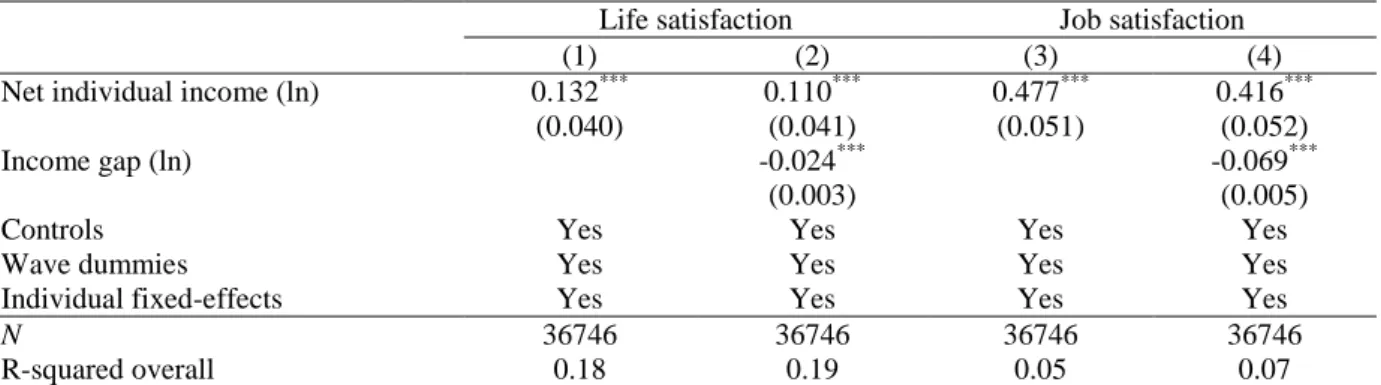
Table 1 displays the results for job and life satisfaction. For both dependent variables, we first estimate a baseline specification with income and the basic controls and then add the income gap in a second specification.

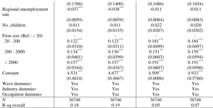
The estimated coefficients on income are significant for both job and life satisfaction in the baseline specification (columns 1 and 3), with (perhaps unsurprisingly) a stronger effect on job satisfaction. The results with respect to the other control variables are very standard in the literature, and the full table of results is relegated to Appendix Table A3. Compared to the married, those who are separated or divorced are less satisfied with their life, while there is no difference regarding job satisfaction. Education has no significant impact on life satisfaction; however, we do find that higher-educated individuals are less satisfied with their jobs, which may well reflect occupational aspirations and job-related stress.8 General health, as self-reported by respondents, is strongly positively correlated with both measures of satisfaction.9 Higher annual hours are associated with lower job satisfaction. Individuals in East Germany are significantly less satisfied with their jobs. Firm size has a positive effect on both job and life satisfaction. Last, the regional unemployment rate is estimated to significantly reduce life satisfaction, which is a common finding in the literature.

7

Clustering at the individual level does not change the nature of any of our results.

8

It should be remembered that these are fixed-effect regressions. Education does not vary that much within individual over time, making the interpretation of the estimated education coefficients a little more difficult.

9

7

The fair-income gap is significantly correlated with both job and life satisfaction. Those whose pay is unfair report significantly lower job and life satisfaction compared to individuals who perceive their income as fair. An individual with the sample mean levels of income and fair income (of 1500 and 2100 respectively) reports a level of life satisfaction that is 0.15 points lower than the same individual when their income is considered to be fair.10 The analogous effect on job satisfaction is 0.44.

Table 1 – The fair income gap and life and job satisfaction

Life satisfaction Job satisfaction

(1) (2) (3) (4)

Net individual income (ln) 0.132*** 0.110*** 0.477*** 0.416***

(0.040) (0.041) (0.051) (0.052)

Income gap (ln) -0.024*** -0.069***

(0.003) (0.005)

Controls Yes Yes Yes Yes

Wave dummies Yes Yes Yes Yes

Individual fixed-effects Yes Yes Yes Yes

N 36746 36746 36746 36746

R-squared overall 0.18 0.19 0.05 0.07

Notes: These are linear models with individual fixed effects. ***=p<0.01; **=p<0.05; *=p<0.10. Standard errors in parentheses are clustered at the region*year level. Income gap (ln) = ln(fair income - income). Additional controls: age dummies, marital status, education, number of children, health status, hours worked, regional unemployment rate, firm size, industry and occupation dummies and individual fixed-effects.

Our second type of well-being measure refers to affect. We show results separately for positive affect (the frequency of feeling happy), and for negative affect (the average frequency of feeling sad, angry and worried). These measures are not available in 2005, so we have one wave less than for the satisfaction analyses. Tables 2 and 3 show the estimates on emotional well-being (the full list of estimated coefficients appears in Appendix Table A4).

Income is insignificant for both aggregate affects,11 while the gap between fair and actual income is significantly correlated with both, increasing the average frequency of feeling sad, angry and worried, and reducing the frequency of happiness.

Looking at the three negative affects separately, we can see that this result is driven by the effect of unfairness on anger and, to a lesser extent, sadness (see Table 3). The effect of fairness on anger confirms what has been suggested in the literature on fairness and reciprocity that the punishment of unfair treatment, in the form for example of less effort or negative reciprocity, is due to feelings of dissatisfaction and anger. In the disaggregated

10

As the log of the gap of 600 here (2100-1500) is 6.4, to be multiplied by the income gap coefficient in Table 2.

11 _{Kahneman and Deaton (2010) use data on US respondents to the Gallup-Healthways Well-Being Index to}

show that income is more strongly correlated with a cognitive/evaluative measure of subjective well-being (the Cantril Ladder) than with positive and negative affect. In the cross-country regressions of Gallup World Poll data in Layard et al. (2012), GDP per capita is correlated with neither positive nor negative affect once controls are introduced (but is correlated with the Cantril Ladder: see their Table 3.1, page 65).

8

results, we also note that the frequency of feeling worried is significantly negatively correlated with the absolute level of income while fairness considerations do not play any role. The size of the marginal effect of log income on worry is notably larger than the size of the log income gap on the other affects.

Table 2 – Effect of fair income on emotional well-being

Positive affects(a) Negative affects(b)

(1) (2) (3) (4)

Net individual income (ln) 0.007 0.003 -0.018 -0.013

(0.020) (0.021) (0.016) (0.016)

Income gap (ln) -0.006*** 0.006***

(0.002) (0.002)

Controls Yes Yes Yes Yes

Wave dummies Yes Yes Yes Yes

Individual fixed-effects Yes Yes Yes Yes

N 30596 30596 30596 30596

R-squared overall 0.06 0.07 0.07 0.07

Notes: (a) Frequency of feeling happy; (b) Average of frequency of feeling sad, angry and worried. Income gap (ln) = ln(fair income - income). These are linear models with fixed effects. ***=p<0.01; **=p<0.05; *=p<0.10. Standard errors in parentheses are clustered at the region*year level. Additional controls: age, marital status, education, number of children, health status, hours worked, regional unemployment rate, firm size, industry and occupation dummies, and individual fixed-effects.

Table 3 – Effect of fair income on positive and negative affect

Happy Sad Angry Worried

Net individual income (ln) 0.003 0.013 0.001 -0.053***

(0.021) (0.026) (0.024) (0.019)

Income gap (ln) -0.006*** 0.004* 0.016*** -0.002

(0.002) (0.002) (0.003) (0.002)

Controls Yes Yes Yes Yes

Time effects Yes Yes Yes Yes

Individual fixed-effects Yes Yes Yes Yes

N 30596 30596 30596 30596

R-sq overall 0.07 0.05 0.04 0.04

Notes: These are linear models with fixed effects. ***=p<0.01; **=p<0.05; *=p<0.10. Standard errors in parentheses clustered at region*year level. Additional controls: age, marital status, education, number of children, health status, hours worked, regional unemployment rate, firm size, industry and occupation dummies, and individual fixed-effects.

4. Unfair income and the probability of quitting the job

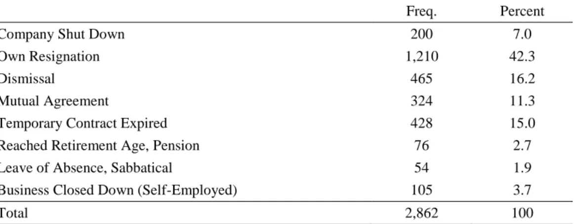
We now turn from subjective to objective outcomes, and estimate the relationship between unfair income and the probability of quitting the job. We relate the information on unfair income to the probability of quitting the job over the next year. We define a job quit as a job change that was caused by the worker leaving the job intentionally (i.e. resigning). About seven percent of employees in the 2005, 2007, 2009, 2011 and 2013 waves separate from their job over the next year; 42% of these separations come about from the worker resigning (see Appendix Table A5). We create a dummy variable for the respondent quitting

9

their job and use this as the dependent variable to estimate the relationship between fairness and job quitting.

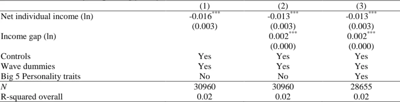
The results appear in Table 4 (the full table of coefficients appears in Appendix Table A6). We estimate linear probability models (the results using probit models are similar and are available upon request). Column 1 contains the results including only income and the other controls; column 2 then adds the gap between fair and actual income; and column 3 is the same model as in column 2 but includes the Big 5 personality traits.12 As almost no-one quits more than once over these five waves, we cannot introduce individual fixed effects; our use of personality traits helps to control for unobserved differences between individuals.

As expected, income reduces job quits. In column 2, we find a significant effect of unfairness on the probability of quitting. Income remains significant here, but with a smaller estimated coefficient. The results in column 2 are robust to the inclusion of personality traits in column 3. Given the small proportion of people quitting their job from one year to another (about 3% on average in the overall period), these effects are quite large: an individual with the mean income gap of 600 has a quit probability that is 1.3 percentage points higher than the same individual with a fair income.13

Table 4 – Probability of quitting job by t+1

(1) (2) (3)

Net individual income (ln) -0.016*** -0.013*** -0.013***

(0.003) (0.003) (0.003)

Income gap (ln) 0.002*** 0.002***

(0.000) (0.000)

Controls Yes Yes Yes

Wave dummies Yes Yes Yes

Big 5 Personality traits No No Yes

N 30960 30960 28655

R-squared overall 0.02 0.02 0.02

Notes: Income gap (ln)= ln(fair income - income). These are cross-section linear probability models. Standard errors in parentheses are clustered at the region*year level. Controls: gender, age dummies, education, marital status, hours work, East, regional unemployment rate, number of children, health, firm size, and industry, occupation and year dummies. ***=p<0.01; **=p<0.05; *=p<0.10.

12 _{These are extraversion, agreeableness, openness, neuroticism, and conscientiousness. They are available in the}

SOEP dataset in three of the five waves we use in the paper, namely 2005, 2009 and 2013. We assume that personality traits are stable over a two-year period and impute the values for the 2007 and 2011 waves from the observations in the preceding waves.

10 5. Additional results: subgroup analysis and comparison income

In this last section we first consider heterogeneity in the effect of fairness considerations on well-being (life satisfaction, job satisfaction and anger) and quits with respect to two individual characteristics: gender and income. We then turn to the relationship between unfair income and the measures of relative income that have often been estimated in the well-being literature.

A large literature has documented a gender gap in income. We might therefore expect women to perceive their income as less fair than do men, although our summary statistics actually reveal no difference in the percentage of males and females perceiving their income as unfair. To see whether unfairness affects men and women differently, we introduce an interaction between gender and the income gap into our regressions: Table 5 displays the results. This interaction term attracts a negative significant coefficient in the life-satisfaction regression: men's well-being is more affected by unfairness than is that of women. This may reflect gender differences in preferences over competition, with women perhaps reacting less to competitive environments than do men (see Gneezy et al., 2003, and Croson and Gneezy, 2009, for example). There is no significant gender difference for the other well-being variables or for job quits (either with an interaction term in column 8, or in separate regressions in columns 9 and 10).

The second characteristic is income. The emotional and behavioural consequences of fairness may well differ along the income distribution. Shaw and Gupta (2001) show, for example, that individuals in financial need, defined as those with children, married, and without alternative sources of income, are less likely to quit their jobs because they are economically dependent, but they suffer from greater dissatisfaction and depression. We here ask whether those in the bottom half of the income distribution have less economic independence than those in the top half.14 The results including an interaction term between the income gap and a dummy for being poor are shown in Table 6.

In line with Shaw and Gupta (2001), we find that the job satisfaction of those in the bottom half of the income distribution is more affected by income unfairness.15 There is also a greater effect of unfairness on job quits for the poor. Regarding our second type of well-being

14

Using an index of financial need based on single-parent household, level of savings and financial worries did not produce significant results.

15

In Schneider (2012), fairness perceptions are measured by comparing what respondents say they think individuals in a certain number of occupations earn to what the same respondents say that these individuals should earn. This produces an individual measure of the fairness of the income distribution. Schneider finds that more unfairness is associated with lower life satisfaction, and that this correlation is stronger for those with higher incomes.

11

measure, individual affects, there is a significant effect only for sadness, which is less affected by income unfairness.

Table 5 - Fair income and gender Life

satisfaction

Job satisfaction

Happy Sad Angry Worried Job quit Job quit Males Job quit Females Net individual income (ln) 0.108** 0.413*** 0.003 0.012 0.001 -0.053*** -0.013*** -0.020*** -0.012*** (0.042) (0.052) (0.021) (0.026) (0.024) (0.019) (0.003) (0.005) (0.004) Income gap (ln) -0.015*** -0.060*** -0.008*** 0.007** 0.015*** 0.001 0.002*** 0.002*** 0.002*** (0.004) (0.008) (0.003) (0.003) (0.003) (0.003) (0.000) (0.000) (0.000) Income gap*male -0.016*** -0.015 0.003 -0.005 0.002 -0.004 -0.000 (0.005) (0.009) (0.003) (0.004) (0.005) (0.004) (0.001)

Controls Yes Yes Yes Yes Yes Yes Yes Yes Yes

Year dummies Yes Yes Yes Yes Yes Yes Yes Yes Yes

Individual fixed-effects

Yes Yes Yes Yes Yes Yes Yes Yes Yes

N 36746 36746 30596 30596 30596 30596 30960 15921 15039 R-sq overall 0.19 0.07 0.07 0.05 0.04 0.05 0.02 0.02 0.02

Notes: ***=p<0.01; **=p<0.05; *=p<0.10. Standard errors in parentheses are clustered at the region*year level. Controls: age dummies, educational level, marital status, hours work, East Germany, regional unemployment rate, number of children, health, and firm size.

Table 6 – Fair income and poor Life

satisfaction

Job satisfaction

Happy Sad Angry Worried Job Quit Job quit Poor Job quit Non Poor Net individual income (ln) 0.080* 0.401*** 0.001 0.019 -0.000 -0.055** -0.011*** -0.013** -0.005 (0.041) (0.058) (0.021) (0.027) (0.025) (0.021) (0.004) (0.005) (0.005) Income gap (ln) -0.026*** -0.060*** -0.009*** 0.007** 0.019*** -0.000 0.001** 0.003*** 0.001*** (0.003) (0.006) (0.002) (0.003) (0.004) (0.002) (0.000) (0.001) (0.000) Income gap*poor 0.007 -0.019** _{0.006 -0.007}* _{-0.007 -0.003 0.002}** (0.005) (0.008) (0.004) (0.004) (0.004) (0.003) (0.001) Poor (1 if Income<median) -0.086** -0.008 -0.014 0.028 0.007 -0.002 0.001 (0.033) (0.051) (0.020) (0.020) (0.024) (0.030) (0.003)

Controls Yes Yes Yes Yes Yes Yes Yes Yes Yes

Year dummies Yes Yes Yes Yes Yes Yes Yes Yes Yes

Individual fixed-effects

Yes Yes Yes Yes Yes Yes Yes Yes Yes

N 36746 36746 30596 30596 30596 30596 30960 14909 16051 R-sq overall 0.19 0.07 0.07 0.05 0.04 0.04 0.02 0.02 0.02

Notes: ***=p<0.01; **=p<0.05; *=p<0.10. Standard errors in parentheses are clustered at the region*year level. Controls: gender, age dummies, educational level, marital status, hours work, East Germany, regional unemployment rate, number of children, health, and firm size. “Poor” here refers to being in the bottom half of the income distribution.

We end this sub-section by asking if the effects of unfairness actually reflect the comparison/relative income effects that have been highlighted in the existing literature. Given our limited number of survey years, we use as a comparison group all individuals in the same age group. We then add this regressor to the specification above in Table 1: the results appear in Table 7. Columns (1) and (4) reproduce the corresponding models of Table 1 for ease of

12

comparison. Both fair income and comparison income have independent negative effects on subjective well-being, but the fair-income estimated coefficient in column (3), when comparison income is controlled for, is identical to that in column (1). The R-squared statistics suggest that fair income fits the well-being data better than does comparison income. We perform a similar analysis for the probability of job quitting. As is evident from Table 8, comparison income does not explain job quitting, whereas the perception of unfair income does.

Table 7 – The fair income gap, the mean reference income and life and job satisfaction

Life satisfaction Job satisfaction

(1) (2) (3) (4) (5) (6)

Net individual income (ln) 0.110*** 0.134*** 0.113*** 0.416*** 0.483*** 0.421***

(0.041) (0.040) (0.041) (0.052) (0.051) (0.052)

Income gap (ln) -0.024*** -0.024*** -0.069*** -0.069***

(0.003) (0.003) (0.005) (0.005)

Mean ref. income (ln) -0.889** -0.841** -1.705*** -1.566***

(0.389) (0.391) (0.524) (0.529)

Controls Yes Yes Yes Yes Yes Yes

Wave dummies Yes Yes Yes Yes Yes Yes

Individual fixed-effects Yes Yes Yes Yes Yes Yes

N 36746 36746 36746 36746 36746 36746

R-squared overall 0.19 0.18 0.19 0.07 0.05 0.07

Notes: These are linear models with individual fixed effects. ***=p<0.01; **=p<0.05; *=p<0.10. Standard errors in parentheses are clustered at the regional*year level. Income gap=ln(fair income-income). The mean reference income is estimated as the average income of individuals in the same age class. Additional controls: age dummies, marital status, education, number of children, health status, hours worked, regional unemployment rate, firm size, industry and occupation dummies and individual fixed-effects.

Table 8: Probability of quitting job in t+1 and mean reference income

(1) (2) (3) (3)

Net individual income (ln) -0.013*** -0.013*** -0.013*** -0.013***

(0.003) (0.003) (0.003) (0.003)

Income gap (ln) 0.002*** 0.002*** 0.002*** 0.002***

(0.000) (0.000) (0.000) (0.000)

Mean ref. income (ln) 0.070 0.057

(0.110) (0.102)

Controls Yes Yes Yes Yes

Wave dummies Yes Yes Yes Yes

Big 5 Personality traits No Yes No Yes

N 30960 28655 _{30960 28655}

R-sq overall 0.02 0.02 _{0.02 0.02}

Notes: Income gap (ln)= ln(fair income - income). The mean reference income is estimated as the average income of individuals in the same age class. These are cross-section linear probability models. Standard errors in parentheses are clustered at the region*year level. Controls: gender, age dummies, education, marital status, hours work, East, regional unemployment rate, number of children, health, firm size, and industry, occupation and year dummies. ***=p<0.01; **=p<0.05; *=p<0.10.

13 6. Conclusions

This paper has considered how income is related to labour-market outcomes in large-scale panel survey data. Our results suggest that the absolute level of income is not a sufficient statistic to predict well-being or behaviour. As has been emphasised in previous experimental work, there is an independent role for fairness. The gap between what individuals receive and what they consider to be fair systematically predicts their job and life satisfaction in panel regressions; it also predicts measures of positive and negative affect. We in particular show that happiness, sadness and especially anger are correlated with the income gap (and are uncorrelated with individual income). On the contrary, worry is correlated with absolute income, but not with the income gap. Moving onto objective outcomes, workers are more likely to quit their job if they perceive their income as unfair, conditional on the level of income received.

Fairness then drives both well-being and behaviour. The complete understanding of this phenomenon requires knowledge of where fairness evaluations come from. It is tempting to consider the latter as being at least partly influenced by general movements in income inequality or macroeconomic conditions. However, with comparisons being in the majority to work colleagues, some part of fairness concerns can likely directly be affected by the firm. In this context, it might be useful to think about wage secrecy: Are fairness concerns harmed by the provision of information on the actual structure of pay (as in Card et al., 2012), or does this provision rather actually correct erroneous perceptions? The relationship between the actual distribution of income and what individuals believe it to be16 will likely continue to be an area of continuing interest for academic research.

16

14 References

Akerlof, G.A., 1982. Labor contracts as partial gift exchange. Quarterly Journal of

Economics 97, 543-569.

Akerlof, G.A., Yellen, J.L., 1990. The fair wage-effort hypothesis and unemployment.

Quarterly Journal of Economics 105, 255-283.

Ben-Shakhar, G., Bornstein, G., Hopfensitz, A., van Winden, F., 2007. Reciprocity and emotions in bargaining using physiological and self-report measures. Journal of

Economic Psychology 28, 314-323.

Bewley, T.F., 1999. Why wages don't fall during a recession. Harvard University Press. Blinder, A.S., Choi, D., 1990. A Shred of Evidence on Theories of Wage Stickiness.

Quarterly Journal of Economics 105, 1003-1015.

Bosman, R., Van Winden, F., 2002. Emotional hazard in a power‐to‐take experiment.

Economic Journal 112, 147-169.

Card, D., Mas, A., Moretti, E., Saez, E. 2012. Inequality at Work: The Effect of Peer Salaries on Job Satisfaction. American Economic Review 102, 2981-3003.

Clark, A.E., 2003. Unemployment as a social norm: Psychological evidence from panel data.

Journal of Labor Economics 21, 323-351.

Clark, A.E., 2015. What makes a good job? Job quality and job satisfaction. IZA World of

Labor, Article 215.

Clark, A.E., 2016. SWB as a Measure of Individual Well-being. In M. Adler and M. Fleurbaey (Eds.), Oxford Handbook of Well-Being and Public Policy. Oxford: Oxford University Press.

Clark, A.E., D'Ambrosio, C. 2015. Attitudes to Income Inequality: Experimental and Survey Evidence. In A. Atkinson and F. Bourguignon (Eds.), Handbook of Income Distribution

Volume 2A. Amsterdam: Elsevier.

Clark, A.E., Masclet, D., Villeval, M.-C., 2010. Effort and Comparison Income. Industrial

and Labor Relations Review 63, 407-426.

Clark, A.E., Oswald, A.J., 1996. Satisfaction and comparison income. Journal of Public

Economics 61, 359-381.

Clark, A.E., Senik, C., 2010. Who compares to whom? The anatomy of income comparisons in Europe. Economic Journal, 120, 573-594.

Cohn, A., Fehr, E., Goette, L., 2014. Fair wages and effort provision: Combining evidence from a choice experiment and a field experiment. Management Science 61, 1-18.

15

Croson, R., Gneezy, U., 2009. Gender differences in preferences. Journal of Economic

Literature 47, 448-474.

Dahlin, M.B., Kapteyn, A., Tassot, C. (2014). Who are the Joneses? CESR-Schaeffer Working Paper No. 2014-004.

Easterlin, R.A., 1974. Does economic growth improve the human lot? Some empirical evidence. In: P.A. David, M.W.R. (Ed.). Nations and households in economic growth:

Essays in Honor of Moses Abramowitz. New York: Academic Press.

Easterlin, R.A., 2001. Income and happiness: Towards a unified theory. Economic Journal 111, 465-484.

Falk, A., Kosse, F., Menrath, I., Verde, P.E., Siegrist, J., 2017. Unfair pay and health.

Management Science, forthcoming.

Fehr, E., Gächter, S., 2000. Fairness and retaliation: The economics of reciprocity. Journal of

Economic Perspectives 14, 159-181.

Fehr, E., Kirchsteiger, G., Riedl, A., 1993. Does fairness prevent market clearing? An experimental investigation. Quarterly Journal of Economics 108, 437-459.

Ferrer-i-Carbonell, A., 2005. Income and well-being: an empirical analysis of the comparison income effect. Journal of Public Economics 89, 997-1019.

Frederick, S., Loewenstein, G., 1999. Hedonic adaptation. In: D. Kahneman, E. Diener, and N. Schwarz, (Eds.). Well-being: The Foundations of Hedonic Psychology. New York: Russel Stage Foundation, p. 302-329.

Gneezy, U., Niederle, M., Rustichini, A., 2003. Performance in competitive environments: Gender differences. Quarterly Journal of Economics 118, 1049-1074.

Goerke, L., and Pannenberg, M., 2015. Direct Evidence for Income Comparisons and Subjective Well-Being across Income Groups. Economics Letters, 137, 95-101.

Kahneman, D., Deaton, A., 2010. High income improves evaluation of life but not emotional well-being. Proceedings of the National Academy of Science, 107, 16489–16493.

Layard, R., Clark, A.E., Senik, C. 2012. The causes of happiness and misery. In J. Helliwell, R. Layard, and J. Sachs (Eds.), World Happiness Report 2012. New York: Columbia Earth Institute.

Long, A. 2005. Happily Ever After? A Study of Job Satisfaction in Australia. Economic

Record, 81, 303-321.

Luttmer, E.F., 2005. Neighbors as negatives: Relative earnings and well-being. Quarterly

16

Mathewson, S.B., 1969. Restriction of output among unorganized workers, 2nd ed. Southern Illinois University Press, Carbondale, IL.

McBride, M., 2010. Money, happiness, and aspirations: An experimental study. Journal of

Economic Behavior & Organization 74, 262-276.

Pfeifer, C. 2015. Unfair Wage Perceptions and Sleep: Evidence from German Survey Data.

Schmollers Jahrbuch, 135, 413-428.

Pfeifer, C., 2017. ‘Have You Felt Angry Lately?’: A Note On Unfair Wage Perceptions And The Negative Emotion Of Anger. Bulletin of Economic Research, forthcoming.

Pillutla, M.M., Murnighan, J.K., 1996. Unfairness, anger, and spite: Emotional rejections of ultimatum offers. Organizational behavior and human decision processes 68, 208-224. Schneider, S.M., 2012. Income inequality and its consequences for life satisfaction: what role

do social cognitions play? Social Indicators Research, 106, 419–438.

Shaw, J.D., Gupta, N., 2001. Pay fairness and employee outcomes: Exacerbation and attenuation effects of financial need. Journal of Occupational and Organizational

Psychology 74, 299-320.

Stutzer, A., 2004. The role of income aspirations in individual happiness. Journal of

17 Appendix

Table A1 - Percentage of respondents considering their income unfair, average amount of fair income and income gap (fair income – income) by population subgroup

Income is Unfair (%) Mean Fair Income Gap from Actual Income (%)

Gender

Female 37.2 1703.7 529.6 (58.3)

Male 37.6 2537.1 753.4 (49.5)

Education

Less than high school 40.8 1607.6 485.6 (64.4)

High school 39.3 1933.3 561.5 (51.9)

More than high school 31.7 2926.5 945.8 (54.1)

Age 25-35 40.5 1865.0 534.9 (53.2) 36-45 35.7 2152.9 628.6 (51.6) 46-55 37.5 2248.3 707.2 (54.3) 56-65 34.6 2298.1 725.2 (57.5) West/East Germany West 33.5 2239.6 655.3 (48.8) East 50.4 1903.7 623.9 (64.7) Year 2005 32.9 2092.5 566.7 (45.4) 2007 42.3 2193.2 645.0 (50.2) 2009 36.8 2041.7 608.1 (56.5) 2011 36.8 2144.1 683.9 (57.2) 2013 37.8 2191.1 711.7 (58.5) Total sample 37.4 2135.5 645.5 (53.7)

Table A2 - Descriptive statistics

Mean Std. Dev. Min Max N

Gender (male) 0.51 0.50 0 1 39537

Age (ref.: <35) 8551

36-45 0.30 0.46 0 1 11889

46-55 0.32 0.47 0 1 12572

>55 0.17 0.37 0 1 6525

Education level (ref.: <High school) 3166

=High school 0.63 0.48 0 1 24824

>High school 0.29 0.45 0 1 11160

Marital status (ref.: married) 25414

Single 0.22 0.41 0 1 8575

Widowed 0.02 0.13 0 1 628

Divorced/separated 0.12 0.33 0 1 4884

Ind. Monthly income (ln) 7.26 0.7 3 11 39537

Income gap (ln) 2.08 2.93 0 11 39537

Unfair income 0.34 0.47 0 1 39537

Health status 3.52 0.84 1 5 39482

18

Annual hours worked/100 19.55 7.19 0 62 39537

East Germany 0.22 0.42 0 1 39537

Firm size (ref.: <20) 8836

20-200 0.29 0.46 0 1 11569

200-2000 0.22 0.42 0 1 8774

>2000 0.26 0.44 0 1 10039

Regional unemployment rate 7.91 3.88 3 21 39537

Job quit 0.03 0.17 0 1 39428 Life satisfaction 7.14 1.60 0 10 38618 Job satisfaction 7.01 1.97 0 10 38136 Happy 3.56 0.81 1 5 31786 Sad 2.31 0.99 1 5 31783 Angry 2.93 0.97 1 5 31800 Worried 1.89 0.9 1 5 31760

Big 5 Personality traits

Extraversion 14.53 3.39 3 21 36528

Agreeableness 16.05 2.88 3 21 36513

Conscientiousnes 14.50 1.81 3 21 36497

Neuroticism 11.32 3.59 3 21 36523

Openness 13.45 3.48 3 21 36442

Table A3 – Effect of fair income on life and job satisfaction. Full table.

Life satisfaction Job satisfaction

(1) (2) (3) (4)

Net individual income (ln) 0.132*** 0.110*** 0.477*** 0.416***

(0.0403) (0.0412) (0.0511) (0.0519) Income gap (ln) -0.024*** -0.069*** (0.0027) (0.0048) Age (Ref.: 25-35) Age 36-45 -0.034 -0.037 0.107** 0.100** (0.0372) (0.0371) (0.0472) (0.0467) Age 46-55 -0.039 -0.039 0.160** 0.160** (0.0463) (0.0460) (0.0648) (0.0640) Age >55 0.029 0.028 0.155* 0.151* (0.0554) (0.0553) (0.0837) (0.0823)

Education level (Ref.: <High school) - - - - =High school 0.003 0.008 -1.406*** -1.391*** (0.3207) (0.3204) (0.3206) (0.3078) >High school -0.122 -0.096 -1.350*** -1.277*** (0.3360) (0.3343) (0.3330) (0.3240)

Marital status (Ref.: Married) - - - - Single -0.025 -0.023 -0.033 -0.028 (0.0368) (0.0363) (0.0632) (0.0613) Widowed -0.498** -0.514*** 0.314* 0.268 (0.1932) (0.1928) (0.1847) (0.1847) Divorced/Separated -0.112** -0.108** 0.003 0.014 (0.0430) (0.0433) (0.0593) (0.0594) Health status 0.449*** 0.446*** 0.398*** 0.390*** (0.0122) (0.0122) (0.0170) (0.0173)

No. hours worked/100 -0.002 -0.001 -0.017*** -0.013***

(0.0019) (0.0019) (0.0025) (0.0026)

19 (0.1396) (0.1400) (0.1686) (0.1654) Regional unemployment rate -0.037*** -0.038*** -0.011 -0.011 (0.0059) (0.0059) (0.0084) (0.0083) No. children 0.011 0.011 -0.022 -0.020 (0.0154) (0.0155) (0.0207) (0.0202)

Firm size (Ref.: < 20) - - - -

20 - 200 0.122*** 0.123*** 0.181*** 0.184*** (0.0310) (0.0311) (0.0499) (0.0497) 200 - 2000 0.134*** 0.136*** 0.151** 0.159*** (0.0401) (0.0399) (0.0603) (0.0594) > 2000 0.157*** 0.157*** 0.191*** 0.191*** (0.0344) (0.0347) (0.0607) (0.0596) Constant 4.531*** 4.677*** 4.509*** 4.933*** (0.4624) (0.4667) (0.6006) (0.5766)

Wave dummies Yes Yes Yes Yes

Industry dummies Yes Yes Yes Yes

Occupation dummies Yes Yes Yes Yes

N 36746 36746 36746 36746

R-sq overall 0.18 0.19 0.05 0.07

Notes: Linear models with fixed effects. ***=p<0.01; **=p<0.05; *=p<0.10. Standard errors in parentheses are clustered at the region*year level. Source: SOEP, waves 2005, 2007, 2009, 2011 and 2013.

Table A4 – Effect of fair income on emotional well-being. Full table.

Positive affects Negative affects

(1) (2) (3) (4)

Net individual income (ln) 0.007 0.003 -0.018 -0.013

(0.0203) (0.0207) (0.0157) (0.0153) Income gap (ln) -0.006*** 0.006*** (0.0019) (0.0016) Age (Ref.: 25-35) - - - - Age 36-45 -0.033 -0.034 0.004 0.005 (0.0260) (0.0261) (0.0186) (0.0186) Age 46-55 0.006 0.006 0.012 0.012 (0.0303) (0.0304) (0.0268) (0.0267) Age >55 0.008 0.008 0.033 0.034 (0.0385) (0.0386) (0.0302) (0.0301)

Education level (Ref.: <High school) - - - -

=High school 0.277 0.279 -0.037 -0.039

(0.2776) (0.2789) (0.1528) (0.1530)

>High school 0.245 0.253 -0.095 -0.103

(0.2565) (0.2578) (0.1676) (0.1680)

Marital status (Ref.: Married) - - - -

Single -0.011 -0.011 -0.039 -0.039 (0.0236) (0.0236) (0.0248) (0.0250) Widowed -0.411*** -0.415*** 0.439*** 0.443*** (0.1104) (0.1103) (0.0770) (0.0778) Divorced/Separated 0.015 0.016 0.064** 0.063** (0.0342) (0.0342) (0.0290) (0.0290) Health status 0.146*** 0.145*** -0.176*** -0.176*** (0.0067) (0.0067) (0.0065) (0.0064)

No. hours worked/100 0.000 0.000 0.002* 0.002*

(0.0012) (0.0012) (0.0011) (0.0011)

East Germany -0.039 -0.037 0.077 0.075

(0.0666) (0.0666) (0.0617) (0.0619)

Regional unemployment rate 0.001 0.001 0.016*** 0.016***

(0.0044) (0.0044) (0.0034) (0.0034)

No. children -0.004 -0.004 -0.031** -0.031**

20

Firm size (Ref.: < 20) - - - -

20 - 200 0.013 0.013 -0.003 -0.004 (0.0229) (0.0230) (0.0186) (0.0187) 200 - 2000 -0.000 0.001 -0.025 -0.026 (0.0243) (0.0244) (0.0200) (0.0199) > 2000 -0.037 -0.036 -0.012 -0.012 (0.0259) (0.0260) (0.0213) (0.0214) Constant 2.655*** 2.688*** 3.154*** 3.121*** (0.3023) (0.3039) (0.2596) (0.2536)

Wave dummies Yes Yes Yes Yes

Industry dummies Yes Yes Yes Yes

Occupation dummies Yes Yes Yes Yes

N 30596 30596 30596 30596

R-sq overall 0.06 0.07 0.07 0.07

Notes: Linear models with fixed effects. ***=p<0.01; **=p<0.05; *=p<0.10. Standard errors in parentheses are clustered at the region*year level. Source: SOEP, waves 2007, 2009, 2011 and 2013.

Table A5 – Reason for job termination

Freq. Percent

Company Shut Down 200 7.0

Own Resignation 1,210 42.3

Dismissal 465 16.2

Mutual Agreement 324 11.3

Temporary Contract Expired 428 15.0

Reached Retirement Age, Pension 76 2.7

Leave of Absence, Sabbatical 54 1.9

Business Closed Down (Self-Employed) 105 3.7

Total 2,862 100

Table A6 - Probability of quitting job by t+1. Full Table

(1) (2) (3)

Net individual income (ln) -0.016*** -0.013*** -0.013***

(0.0032) (0.0032) (0.0031) Income gap (ln) 0.002*** 0.002*** (0.0004) (0.0004) Male 0.004* 0.004* 0.004* (0.0021) (0.0021) (0.0021) Age (Ref.: 25-35) - - - Age 36-45 -0.021*** -0.020*** -0.018*** (0.0032) (0.0032) (0.0036) Age 46-55 -0.030*** -0.030*** -0.028*** (0.0035) (0.0035) (0.0036) Age >55 -0.039*** -0.039*** -0.037*** (0.0034) (0.0034) (0.0038)

Education level (Ref.: < High school) - - -

= High school -0.000 -0.000 0.000

(0.0035) (0.0035) (0.0036)

> High school 0.012*** 0.011*** 0.011***

(0.0040) (0.0040) (0.0040)

Marital status (Ref.: Married) - - -

Single 0.003 0.003 0.003

(0.0033) (0.0032) (0.0035)

Widowed -0.001 -0.001 0.001

21

Divorced/Separated 0.009*** 0.008*** 0.008***

(0.0029) (0.0028) (0.0031)

Health status 0.003** 0.003*** 0.003**

(0.0011) (0.0011) (0.0012)

No. hours worked/100 0.001** 0.000 0.000

(0.0002) (0.0002) (0.0002)

East Germany -0.009** -0.010*** -0.010***

(0.0034) (0.0034) (0.0037)

Regional unemployment rate 0.000 0.000 -0.000

(0.0004) (0.0004) (0.0005)

No. children 0.002 0.002 0.001

(0.0012) (0.0012) (0.0013)

Firm size (Ref.: < 20) - - -

20 - 200 -0.007*** -0.008*** -0.008*** (0.0026) (0.0026) (0.0030) 200 - 2000 -0.010*** -0.010*** -0.009*** (0.0032) (0.0031) (0.0031) > 2000 -0.009*** -0.009*** -0.009*** (0.0030) (0.0029) (0.0031) Constant 0.082*** 0.064*** 0.044* (0.0228) (0.0225) (0.0226)

Wave dummies Yes Yes Yes

Industry dummies Yes Yes Yes

Occupation dummies Yes Yes Yes

Big 5 Personality Traits No No Yes

N 30960 30960 28655

R-sq overall 0.02 0.02 0.02

Notes: Linear probability models. Standard errors in parentheses are clustered at the region*year level. ***=p<0.01; **=p<0.05; *=p<0.10. Source: SOEP, waves 2005-2014.