Modeling shapes with skeletons : scaffolds & anisotropic convolution

HAL Id: tel-02420728

https://tel.archives-ouvertes.fr/tel-02420728v2

HAL is a multi-disciplinary open access

archive for the deposit and dissemination of sci-entific research documents, whether they are

pub-L’archive ouverte pluridisciplinaire HAL, est destinée au dépôt et à la diffusion de documents scientifiques de niveau recherche, publiés ou non,

Modeling shapes with skeletons : scaffolds & anisotropic

convolution

Alvaro Javier Fuentes Suarez

To cite this version:

Alvaro Javier Fuentes Suarez. Modeling shapes with skeletons : scaffolds & anisotropic convolution. General Mathematics [math.GM]. COMUE Université Côte d’Azur (2015 - 2019), 2019. English. �NNT : 2019AZUR4057�. �tel-02420728v2�

Modélisation de formes à l'aide de

squelettes: échafaudages & convolution

anisotrope

Alvaro Javier FUENTES SUAREZ

AROMATH, Inria Sophia-Antipolis

Présentée en vue de l’obtention du grade de docteur en Mathematiques d’Université Côte d’Azur

Dirigée par : Evelyne Hubert Soutenue le : 27/09/2019

Devant le jury, composé de :

JeanDaniel Boissonnat, Directeur de recherche, INRIA -Université Côte d’Azur

Marie-Paule Cani, Professeur, Ecole Polytechnique Paris-Saclay

Jorg Peters, Professeur, Université de Floride (Etats-Unis) Geraldine Morin, Professeur, Université de Toulouse Marco Livesu, Chercheur, Conseil National de la Recherche d’Italie

Adrien Bousseau, Chargé de recherche, INRIA Université Côte d’Azur

squelettes: échafaudages & convolution

anisotrope

Jury :

Président du jury

M. Jean-Daniel Boisonnant, Directeur de recherche, INRIA Université Côte d’Azur

Rapporteurs

Mme Marie-Paule Cani, Professeur, Ecole Polytechnique Paris-Saclay M. Jorg Peters, Professeur, Université de Floride (Etats-Unis)

Examinateurs

Mme Géraldine Morin, Professeur, Université de Toulouse

M. Marco Livesu, Chercheur, Conseil National de la Recherche d’Italie M. Adrien Bousseau, Chargé de recherche, INRIA Université Côte d’Azur

Directrice de thèse

Résumé

Modélisation

de

formes

à

l’aide

de

squelettes:

échafaudages & convolution anisotrope

Les squelettes se sont révélés être un outil efficace pour modéliser des formes complexes. Ils fournissent une base pour de nombreux processus allant de la modélisation implicite à la déformation et aux animations. Dans ce travail, nous abordons deux sujets liés à la modélisation avec squelette: les maillages quad-dominants à base de squelette et les surfaces lisses implicites générées à partir d’un squelette.

Étant donné un squelette constitué de segments de droite, nous décrivons comment obtenir un maillage quad-dominant d’une surface qui entoure étroitement le squelette et suit sa structure - l’échafaudage. Nous formalisons sous forme de programme linéaire sur les entiers le problème de la construction d’un échafaudage optimal minimisant le nombre total de quads sur le maillage. Nous prouvons la faisabilité du programme linéaire entier pour tout squelette. En particulier, nous pouvons générer ces échafaudages pour des squelettes avec des cycles. Nous montrons également comment obtenir des échafaudages réguliers, c’est-à-dire des échafaudages avec le même nombre de quads autour de chaque segment de droite, et des échafaudages symétrique respectant les symétries du squelette. Des applications à la polygonisation de surfaces implicites à base de squelettes sont également présentées.

Les surfaces de convolution avec des squelettes 1D ont été limitées à des sections normales presque circulaires. La nouvelle formulation que nous présentons ici augmente les possibilités de modélisation car elle permet les sections normales ellipsoïdales. Cette anisotropie est definie pour des courbes squelettalesG1, choisies comme des splines circulaires, en interpolant l’angle de rotation et les trois rayons d’ellipsoïdes donnés, par l’utilisateur, à chaque extrémité de la courbe. Ce modèle léger crée des formes lisses qui nécessitaient auparavant de peaufiner le squelette ou de le compléter avec des pièces 2D. L’invariance par homotetie de notre formulation permet un contrôle fin des rayons et se prête ainsi à approximer une variété de formes. La construction d’un échafaudage est étendue aux squelettes avec des branchesG1. Il se projette sur la surface de convolution pour former un maillage quad-dominant avec un flux d’arrêtes qui longe le squelette.

En plus des deux contributions principales décrites ci-dessus, nous développons d’autres sujets liés aux échafaudages et aux surfaces de convolution. Nous discutons la façon dont les diagrammes de Laguerre sphériques peuvent être utilisés pour améliorer la forme des échafaudages lorsque différents rayons incidents sont autorisés au niveau des articulations, et nous décrivons comment construire des maillages hexaédriques volumétriques pour un modèle basé sur un squelette à partir d’un échafaudage. Nous introduisons également les techniques de Télescopage Créatif pour le calcul par récurrence de formes closes de fonctions de convolution. Enfin, nous présentons PySkelton -une bibliothèque Python pour la modélisation basée sur le squelette qui implémente nos algorithmes et fournit une interface de programmation conviviale pour les académiques.

Mots clé: Modélisation à base de squelettes, surfaces implicites, échafaudages, surfaces de convolution

Abstract

Modeling shapes with skeletons: scaffolds & anisotropic

convolution

Skeletons have proved to be a successful tool in modeling complex shapes. They provide a basis for many processes ranging from implicit modeling, to deformation and animations. In this work we advance in two topics related with skeleton modeling: quad dominant skeleton-based meshes and smooth implicit surfaces generated from a skeleton.

Given a skeleton made of line segments we describe how to obtain a coarse quad mesh of a surface that tightly encloses the skeleton and follows its structure – the scaffold. We formalize as an Integer Linear Program the problem of constructing an optimal scaffold that minimizes the total number of quads on the mesh. We prove the feasibility of the Integer Linear Program for any skeleton. In particular we can generate these scaffolds for skeletons with cycles. We additionally show how to obtain regular scaffolds, i.e. scaffolds with the same number of quad patches around each line segment, and symmetric scaffolds that respect the symmetries of the skeleton. Applications to polygonization of skeleton-based implicit surfaces are also presented.

Convolution surfaces with 1D skeletons have been limited to close-to-circular normal sections. The new formalism we present here increases the modeling freedom since it allows for ellipsoidal normal sections. The new anisotropy forG1skeletal curves, chosen as circular splines, is interpolated from the rotation angles and three radii of ellipsoids at each extremity, given as user input. This lightweight model creates smooth shapes that previously required tweaking the skeleton or supplementing it with 2D pieces. The scale invariance of our formalism achieves excellent radii control and thus lends itself to approximate a variety of shapes. The construction of a scaffold is extended to skeletons withG1branches. It projects onto the convolution surface as a quad mesh with skeleton bound edge-flow.

In addition to the two main contributions described above we develop further topics related to scaffolding and convolution surfaces. We discuss how spherical Laguerre diagrams may be used to improve the scaffold shapes when different incident radii is allowed at joints, and we describe how to construct volumetric hexahedral meshes for a

skeleton-based model starting from a scaffold. We also introduce Creative Telescoping techniques for the computation of closed form formulas through recurrence. Finally we present PySkelton – a Python library for skeleton based modeling that implements our algorithms and provides an academic friendly programming interface.

Keywords: Skeleton-based modeling, implicit surfaces, scaffolds, convolution sur-faces

Contents

I

Scaffolds

18

1 Scaffolding skeletons using spherical Voronoi diagrams: feasibility,

regular-ity and symmetry 19

1.1 Introduction . . . 20

1.1.1 Previous work . . . 21

1.1.2 Contributions . . . 22

1.2 Skeletons & Scaffolds . . . 23

1.3 Existence of scaffolds . . . 25

1.3.1 Locally uniform discretization . . . 25

1.3.2 Standard scaffold . . . 27

1.3.3 Symmetric scaffold . . . 28

1.3.4 Regular symmetric scaffold . . . 31

1.4 Optimal scaffolds . . . 34

1.4.1 Objective function . . . 34

1.4.2 Integer Linear Programming models . . . 35

1.5 Algorithms . . . 36

1.6 Further simplifications of the scaffold . . . 42

1.7 Application to polygonization . . . 44

2 Further topics on scaffolding 47

2.1 Hexahedral meshes . . . 48

2.1.1 Limitations . . . 51

2.2 Laguerre diagrams: controlling the cell size . . . 52

2.2.1 Definition and algorithm variants . . . 52

2.2.2 Limitations . . . 56

2.3 Conclusions . . . 58

II

Convolution surfaces

59

3.2 Discussion on the choice of a kernel . . . 62

3.3 Convolution of regular curves . . . 65

3.4 Line segments and arcs of circle . . . 66

3.5 Varying thickness . . . 66

3.6 Closed form formulas . . . 68

3.7 Numerical integration . . . 68

4 Closed form formulas from recurrence 70 4.1 Creative Telescoping . . . 71

4.1.1 Practical use . . . 73

4.2 Convolution with line segments . . . 74

4.2.1 Integrals for convolution . . . 74

4.2.2 Closed forms through recurrence formulas . . . 75

4.3 Convolution with arcs of circle . . . 76

4.3.1 Rational parametrization . . . 77

4.3.2 Integrals for convolution . . . 78

4.3.3 Closed forms through recurrence formulas . . . 79

4.4 Conclusions . . . 80

5 Anisotropic convolution surfaces 81 5.1 Introduction . . . 82

5.1.1 Related work . . . 83

5.1.2 General overview and contributions . . . 84

5.2 Preliminaries: circular splines and frames . . . 85

5.2.1 Circular splines: approximation of general curves . . . 85

5.2.2 Frames forG1curves . . . 87

5.3 Convolution surfaces: from varying thickness to anisotropy . . . 88

CONTENTS

5.3.2 Anisotropic convolution . . . 90

5.4 Skeleton-driven meshing . . . 99

5.4.1 Scaffolds for circular splines . . . 100

5.4.2 Mesh projection onto the convolution surface . . . 102

5.5 Implementation and Numerical integration . . . 103

5.6 Examples & Applications . . . 104

5.6.1 Skeleton-based modeling . . . 104

5.6.2 Blobtree modeling . . . 104

5.6.3 Shape approximation . . . 106

5.7 Conclusions . . . 111

III

Implementation

112

6.2.2 Anisotropic convolution mesh example . . . 121

6.3 Implementation . . . 122

6.3.1 Integration . . . 122

6.3.2 Ray shooting . . . 123

6.4 Conclusions . . . 124

1 Scaffold construction. . . 12

2 Convolution surfaces . . . 13

3 Anisotropy in convolution surfaces . . . 15

1.1 Recreation of some of the scaffolds used in [Karˇciauskas and Peters, 2016] 20 1.2 Construction of cells . . . 23

1.3 Degenerate cases . . . 24

1.4 Symmetric scaffold . . . 29

1.5 False symmetry . . . 29

1.6 Three-fold rotation symmetry . . . 32

1.7 Complex closed skeletons . . . 32

1.8 Symmetry vs regularity . . . 33

1.9 Symmetric improvements . . . 34

1.10 Cases for the convex hull ofAv . . . 37

1.11 Twisting artifacts . . . 40

1.12 Different radii at joints . . . 41

1.13 Simplification of the equations in the IP. . . 42

1.14 Scaffold with three points per cell . . . 43

1.15 Close-to-coplanar intersection points . . . 44

1.16 Scaffolds for meshing . . . 45

2.1 The hexahedron HQfrom the scaffold quad Q. . . 48

2.2 Hexahedral mesh from scaffold . . . 49

2.3 Stratified hexahedra subdivision . . . 49

2.4 Hexahedra around a joint . . . 50

2.5 Hexahedral meshes for highly symmetric skeletons . . . 51

2.6 Spherical Laguerre diagram to better approximate incident radii . . . . 53

2.7 _{S projected to the plane containing the triangle OA}iAj . . . 55

2.8 Spherical Laguerre diagram examples . . . 57

3.1 Convolution curves based on two parallel segments . . . 63

LIST OF FIGURES

3.3 Convolution curves for a set of segments with power inverse kernel . . . 65

4.1 Rational parametrization of an arc of circle. . . 77

5.1 Convolution surfaces aroundG1circular splines vs polylines . . . 86

5.2 The biarc construction . . . 87

5.3 Biarcs interpolation of a curve . . . 87

5.4 Rotation of frames along spline . . . 88

5.5 Constant metric matrices along a line segment. . . 91

5.6 Ellipsoid representation of the metric matrix . . . 92

5.7 Interpolation of the metric matrix . . . 93

5.8 Anisotropic convolution around a line segment with a combination of twisting and varying thickness . . . 94

5.9 Anisotropic convolution effect on the extremities . . . 94

5.10 Extended modeling capabilities of anisotropic convolution. . . 95

5.11 Auxiliar plot in proof of Proposition 5.3.2 . . . 96

5.12 Radii control in anisotropic convolution . . . 98

5.13 Impact of tangential radii on the surface . . . 99

5.14 The scaffolding method . . . 100

5.15 Meshing with a scaffold . . . 101

5.16 Transporting a vector along a frame . . . 102

5.17 Abstract cage-like surfaces of positive genus . . . 103

5.18 Elk model . . . 104

5.19 Convolution surface around a circular spline approximation of a knot . . 105

5.20 Salamander model . . . 105

5.21 A cup modeled with blobree . . . 106

5.22 Post-processing of skeletonization algorithms output . . . 107

5.23 Semi-automatic approximation of the fertility model . . . 109

5.24 Surface approximation via skeletonization . . . 110

6.1 UML diagram of PySkelton.skeletonsubmodule. . . 115

6.2 UML diagram of PySkelton.fieldsubmodule. . . 116

6.3 Scaffold representing a dragon computed with PySkelton. . . 120

1.1 Integer Linear Program models. . . 36

1.2 Running time of scaffolding implementation . . . 42

1.3 Summary of some scaffolds in this chapter . . . 43

General introduction

This introductory chapter provides an overview of the contributions in this thesis. Since we kept the chapters of this thesis as close as possible to their original publications, more discussion on the state of the art can be found within the individual chapters.

Modeling shapes with skeletons has proved useful in many applications, as discussed in the very good survey in [Tagliasacchi et al., 2016]. A skeleton, made of a set of curves and/or surfaces centered inside a shape, provides a structure that encapsulates some properties of the shape while also being easier to manipulate. In this work we focus on two geometric modeling applications for 1D skeletons: the generation of a surrounding mesh and the construction of an implicit surface. There is special emphasis on the mathematical foundations of the constructions we propose.

Scaffolds. Generally speaking a scaffold is a mesh constructed around a skeleton made of line segments and such that it “follows” the skeleton (see chapters 1 and 2). A simple way to look at a scaffold is as a “thickening” of a 1D skeleton into a surface (see Figure 1). One can also say that a scaffold is a “cage-like” or “truss” structure.

These structures are key steps in many applications. They have been used for artistic purposes [Hart, 2002, Hart, 2008], in architecture [Srinivasan et al., 2005], for modeling [Bærentzen et al., 2012, Panotopoulou et al., 2018], sculpting model-ing [Ji et al., 2010, Wu and Liu, 2012], compatible quadrangulation [Yao et al., 2009], semi-regular quad meshing [Usai et al., 2015], volumetric hexahedral mesh-ing [Livesu et al., 2016], cage generation for posmesh-ing [Casti et al., 2019], and others.

For most applications, quad-dominant scaffolds are desirable, that is scaffolds with a majority of quad patches. The main difficulties in the generation of scaffolds arise from the presence of cycles and high valency joints (nodes where several skeleton pieces meet). As undesired effect we get the presence of spurious patches on the scaffold that are not associated to any piece of the skeleton. Example of methods generating extra quads are those in [Yao et al., 2009] and [Usai et al., 2015]. In [Yao et al., 2009, Figure 4] one can appreciate spurious quads around joints, while in [Usai et al., 2015, Figure 6] the extra quads are due to the presence of a cycle in the skeleton. In [Ji et al., 2010] the extra patches around joints are triangular patches, while [Bærentzen et al., 2012] cannot handle skeletons with cycles.

Figure 1: Scaffold construction.

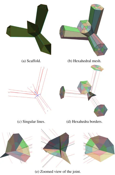
In Chapter 1 we present a method for generating scaffolds that can handle skeletons with cycles. Our method does not create spurious quads around joints, and allows to construct scaffolds that satisfy any group of symmetries of the input skeleton. We construct an optimal scaffold by minimizing the total number of quads in an Integer Linear Programming model, for which we formally prove feasibility. In Chapter 2 we describe how to generate a hexahedral volumetric mesh from the scaffolds we construct. Avoiding spurious quads is not only useful for modeling and post-processes, but the total lack of spurious quads is a key property of our method that made possible the volumetric hexahedral meshing. Also in Chapter 2 we present a variant of our scaffolding method that provides more control over the shape of the scaffolds.

Convolution surfaces. In skeleton-based modeling the user starts with a set of 1D (curves) or 2D (surfaces) objects that serves as skeleton for a shape surrounding it. Surfaces built around a skeleton are very useful since the skeleton provides an intuitive way to manipulate the surface. Several meth-ods have been proposed for the generation of surfaces around 1D skele-tons: sweep surfaces [Requicha, 1980], offset surfaces [Pham, 1992], canal faces [Peternell and Pottmann, 1997], B-Meshes [Ji et al., 2010], and convolution sur-faces [Blinn, 1982, Bloomenthal and Shoemake, 1991, Zanni, 2013] are some of them. Convolution surfaces are specially attractive because they not only add radii information to the skeleton, but also provide a way to blend individual pieces in a smooth way (see Figure 2).

(a) Simple pieces. (b) Complex model. Figure 2: Convolution surfaces

Zhu et al., 2015b], character modeling [Zanni et al., 2011], sketch-based model-ing [Entem et al., 2015, Bernhardt et al., 2008, Zhu et al., 2011, Wither et al., 2009], im-merse modeling in virtual environments [Zhu et al., 2017], and others. More specifically, a convolution surface is an implicit surface defined as a level set of a scalar field, the convolution field, that is obtained by integrating a kernel function over the skeleton. This technique can be used also to model volumes and are suitable to be combined in other implicit modeling frameworks [Pasko et al., 1995, Wyvill et al., 1999].

The mathematical smoothness of the surface obtained depends only on the smooth-ness of the kernel. The kernel function (power inverse, Cauchy, compact sup-port, . . . ) may be selected so as to have closed form expressions for the con-volution functions associated to basic skeleton elements (line segments, triangles, . . . ). The additivity property of integration makes the convolution function inde-pendent of the partition of the skeleton. More general skeletons are then par-titioned and approximated by a set of basic elements. The convolution func-tion for the whole skeleton is obtained by adding the convolufunc-tion funcfunc-tions of the constitutive basic elements. See for instance [Bloomenthal and Shoemake, 1991, Cani and Hornus, 2001, Hornus et al., 2003, Jin and Tai, 2002a, Jin and Tai, 2002b, Jin et al., 2001, Sherstyuk, 1999a, Sherstyuk, 1999b, Zanni, 2013, Zanni et al., 2013].

Line segments are the most commonly used 1D basic skeleton elements. When a skeleton consists of curves with high curvature or torsion, its approximation might require a great number of line segments for the convolution surface to look as intended. Arcs of circles form a very interesting class of basic skeleton elements in the context of convolution. This was already argued in [Jin and Tai, 2002b] for planar skeleton curves. Indeed any space curve can be approximated by circular splines in aG1 fash-ion [Nutbourne and Martin, 1988, Song et al., 2009]. A lower number of basic skeleton elements are then needed to obtain an appealing convolution surface, resulting in better

visual quality at lower computational cost.

To model a wider variety of shapes it is necessary to vary the thick-ness around the skeleton. Several approaches have been suggested: weighted skeletons [Hubert and Cani, 2012, Jin and Tai, 2002a, Jin et al., 2001], varying radius [Hornus et al., 2003], scale invariant integral surfaces [Zanni et al., 2013], the latter two actually providing a more intrinsic formulation.

Closed form formulas, obtained through symbolic computation, have been the tool of choice for evaluating the convolution fields. While general closed form formulas were obtained for weighted line segments in [Hubert and Cani, 2012], there has been a lack of generality in terms of closed form formulas for convolution with varying radius, or scale, over line segments and, even more so, over arcs of circles. A study of the symbolic formulas for power inverse kernels is discussed in Chapter 4 with the use of some advanced computer algebra techniques.

The recurrence formulas for arcs of circle with varying radii or scale present a formidable number of terms. Their numerical evaluation can lead to instabilities. We hence feel we pushed the symbolic approach to its limits. For a more versatile ap-proach we call on numerical integration using the well established quadrature methods implemented in QUADPACK [Piessens et al., 1983].

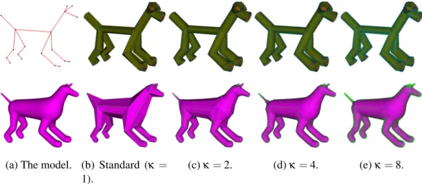
Anisotropy. Standard convolution surfaces around 1D skeletons have circular cross sections. That is also the case for varying radius and scale integral surfaces. This significantly restricts the shapes that can be generated. In Chapter 5 we discuss previous approaches for mitigating this issue and we introduce a new technique to generate anisotropicconvolution surfaces. A simple and intuitive approach to control the shape is also provided. In Figure 3 we illustrate anisotropy in the context of convolution surfaces.

Medial axis, the most intrinsic skeleton, has 2D and 1D elements. Con-volution surfaces around 2D skeletons have been approached in the litera-ture [McCormack and Sherstyuk, 1998, Jin et al., 2008, Hubert, 2012, Zhu et al., 2011, Zanni et al., 2013, Zhu et al., 2017]. While useful, 2D skeletons increase the complexity in the formulas involved as well as on the modeling process for the user. In this thesis we favor the use of 1D skeletons. Anisotropic convolution limits the need of 2D parts by extending the capabilities of convolution around 1D skeletons such that one can mimic the effects of 2D skeletons, as discussed in Chapter 5.

In this work we assume that the modeled surface is topologically consistent with the skeleton. The precise radii control introduced in Chapter 5 allows the user to detect when this is not the case. Consistency between the surface and the skeleton allows to identify a good edge-flow on a surface mesh: when the edges “follow” the 1D skeleton. We explore in Chapter 5, after a brief discussion at the end of Chapter 1, the use of our scaffolds for the meshing of skeleton-consistent implicit surfaces with good edge-flow on the final mesh. For readers interested in a detailed discussion of skeleton-surface topological

(a) Standard convolution. (b) Anisotropic convolution.

Figure 3: Anisotropy in convolution surfaces. In the top row we show the surface and two slicing planes. In the bottom we show the cross sections given by the slicing planes.

consistency in the context of convolution surfaces we refer to [Ma and Crawford, 2008]. PySkelton. Our research results were implemented into a Python library. Our library makes use of established libraries for mathematical programming and numerical analysis: Qhull [Barber et al., 1996] for convex hull computations, GSL [Galassi et al., 2017] and QUADPACK for numerical integration and root finding, and GLPK [Makhorin, 2016] for integer linear programming.

Much of the content of this work has been published and presented in the following papers and venues:

Scaffolding:

• [Fuentes Suárez and Hubert, 2018b] Fuentes Suárez, A. J. and Hubert, E. (2018b). Scaffolding skeletons using spherical Voronoi diagrams: Feasibility, regularity and symmetry. Computer-Aided Design, 102:83–93.

Presented in SPM2018: Solid and Physical Modeling. June 11-13, 2018, Bilbao, Spain.

Topic: full development of the scaffolding algorithm, generation of optimal quad-dominant meshes that respect the symmetries of the skeleton, and with the same number of patches around each line segment (regularity).

• [Fuentes Suárez and Hubert, 2017] Fuentes Suárez, A. J. and Hubert, E. (2017). Scaffolding skeletons using spherical Voronoi diagrams. Electronic Notes in Discrete Mathematics, 62:45–50.

Presented in LAGOS2017: IX Latin and American Algorithms, Graphs, and Optimization Symposium. September 11-15, 2017, CIRM, Marseille, France. Topic: proof of feasibility for the construction of a scaffold (quad dominant mesh that follows the structure of the skeleton) for skeletons made of line segments of any topology.

Extended abstract.

• Poster presentation: Scaffolding skeletons using spherical Voronoi diagrams. FoCM2017: Foundations of Computational Mathematics. July 10-19, 2017, Barcelona, Spain.

Convolution surfaces:

• [Fuentes Suárez et al., 2019] Fuentes Suárez, A. J., Hubert, E., and Zanni, C. (2019). Anisotropic convolution surfaces. Computers & Graphics, 82:106–116. Presented in SMI2019/IGS2019: Shape Modeling International 2019, International Geometry Summit 2019. June 17-22, 2019, Vancouver, Canada.

Topic: An extension to the convolution surfaces technique that increases the modeling freedom. A scaffold-based meshing technique for implicit surfaces around a skeleton is also discussed.

Full content in Chapter 5.

• [Fuentes Suárez and Hubert, 2018a] Fuentes Suárez, A. J. and Hubert, E. (2018a). Convolution surfaces with varying radius: Formulae for skeletons made of arcs of circles and line segments. In Research in Shape Analysis: WiSH2, Sirince, Turkey, AWM, pages 37–60. Springer.

Topic: study of symbolic formulas for convolution surface fields, introduction of Creative Telescoping in the context of closed form formulas for convolution surfaces.

Partial and adapted content in chapters 3 and 4.

• Poster presentation: Anisotropic convolution for modeling 3D smooth shapes around 1D skeletons. 9th International Conference on Curves and Surfaces. June 28-July 4, 2018, Arcachon, France.

As a summary, the contributions in this thesis are: • Scaffolding algorithm and extensions.

• Anisotropic convolution surfaces.

• Meshing of implicit surfaces using scaffolding.

• Python library implementing scaffolding and anisotropic convolution. • Symbolic integral formulas for convolution surfaces through recurrence.

This manuscript is structured as follows. In Chapter 1 we introduce our scaffolding method. In Chapter 2 we discuss potential extensions and generalizations of scaffolding. In Chapter 3 we introduce convolution surfaces. In Chapter 4 we present the closed form formulas for convolution fields. Chapter 5 is devoted to our anisotropic extension of convolution surfaces. Finally in Chapter 6 we present the library we developed with the implementations of the methods and algorithms from chapters 1 and 5. We conclude with some general overviews and comments on future development.

Chapter 1

Scaffolding skeletons using spherical

Voronoi diagrams: feasibility,

regularity and symmetry

This chapter was published in:

[Fuentes Suárez and Hubert, 2018b] Fuentes Suárez, A. J. and Hubert, E. (2018b). Scaffolding skeletons using spherical Voronoi diagrams: Feasibility, regularity and symmetry. Computer-Aided Design, 102:83–93.

An extended abstract version was also published in:

[Fuentes Suárez and Hubert, 2017] Fuentes Suárez, A. J. and Hubert, E. (2017). Scaf-folding skeletons using spherical Voronoi diagrams. Electronic Notes in Discrete Mathe-matics, 62:45–50.

1.1

Introduction

Skeletons are used in 3D graphics for modeling and animating articulated shapes. The user can design a complex shape by sketching a simple geometric object that is the input to a surface generating algorithm. By making changes in the skeleton it is possible to change the shape in an intuitive way. Due to their low dimensional nature, skeletons can serve as an efficient and compact representation of a surface. In this context a skeleton-based mesh generation method is needed.

(a)

(b) (c) (d)

automatic construction

input output

Figure 1.1: Recreation of some of the scaffolds used in [Karˇciauskas and Peters, 2016], automat-ically computed by our method from suitable skeletons.

The idea developed here is to construct a “coarse” quad mesh that tightly follows the structure of the skeleton. Following the terminology of [Panotopoulou et al., 2018] we call this process scaffolding and the corresponding coarse mesh a scaffold. This is used as an intermediate step in many applications. A scaffold can be used to generate a surface, either by subdivision as in [Bærentzen et al., 2012], or as initial patchwork for a spline surface [Blidia et al., 2017, Karˇciauskas and Peters, 2016] (see Figure 1.1). It is used as an intermediate step in the extraction of a quad layout on a given trian-gular mesh [Bærentzen et al., 2014, Usai et al., 2015], and for compatible quadrangula-tion [Yao et al., 2009]. An applicaquadrangula-tion we present here is the polygonizaquadrangula-tion of skeleton-based implicit surfaces into quad-dominant meshes. In particular, we use our method for visualization of convolution surfaces [Bloomenthal and Shoemake, 1991, Zanni, 2013].

1.1. INTRODUCTION

Our main contribution is in the theoretical foundations of an algorithm that computes a scaffold for any skeleton, independently of its topology, and with no user interaction.

In this paper we deal with skeletons made of line segments that do not intersect except at the endpoints, then called joints.

1.1.1

Previous work

One of the earliest ideas for a scaffold construction was to sweep a fixed polygonal cross profile along the segments, stitching the generated quads by means of a convex hull construction at the joints. This idea was first used in [Srinivasan et al., 2005], producing meshes with some triangular faces resulting from the stitching process. For quadrilateral cross profiles B-meshes method [Ji et al., 2010] improved upon this by merging triangles in order to get a quad-dominant mesh. Still the stitching process might leave some triangular patches at the joints.

[Usai et al., 2015] and [Yao et al., 2009] proposed a scaffolding technique that gener-ates a pure-quad mesh by extruding boxes emanating from cubes positioned at the joints. In [Usai et al., 2015] the subdivision of the cubes is modeled with an Integer Linear Program, for which a solution might fail to exist when there are cycles in the skeleton. “Lids” [Usai et al., 2015, Figure 6] are introduced as a workaround. [Yao et al., 2009]

also introduces extra quads around joints [Yao et al., 2009, Figure 4].

The method we propose is based on the Skeleton to Quad-dominant polygonal Mesh (SQM) method in [Bærentzen et al., 2012] which was limited to skeletons without cycles. SQM first defines the mesh points around the joints and then recreate a quad based “tubular” polyhedral surface around each line segment. SQM can be regarded as a three

steps process:

1. Partition the unit sphere centered at the joints into regions, one for each incident line segment.

2. Discretize each region into a cell (as an ordered set of points on its boundary) such that the two cells at the extremities of each line segment are compatible, i.e. have equal number of points. Points on the boundary of two regions are part of the two corresponding cells.

3. Link, in a bijective way, the cells at the extremities of each line segment. These links define the quads on the mesh.

For Step 3, SQM [Bærentzen et al., 2012] defines the links by minimizing the to-tal length of the line segments they define. In Step 2 Bærentzen et al. propose an algorithm for inserting additional vertices on the cells in such a way that the com-patibility constraint is satisfied. Yet this algorithm does not work in the presence of cycles [Bærentzen et al., 2012]. The existence of a possible discretization was actually

not proved. Furthermore there was no analysis on the optimality of SQM with respect to the number of quads in the scaffold.

The partition of the sphere, in Step 1, used in [Bærentzen et al., 2012] can be recog-nized to be a Voronoi diagram on the sphere. [Panotopoulou et al., 2018] introduces a partition of the sphere in quadrangles that makes the compatibility of cells (Step 2) trivial. Yet the partition is not canonical and the convexity of the regions is not guaranteed.

1.1.2

Contributions

Our method follows SQM [Bærentzen et al., 2012] but we address and solve the crux difficulty that represents Step 2 for skeletons of arbitrary topology. We formalize the creation of compatible cells (Step 2) as an Integer Linear Program (IP) that minimizes the total number of quads. We prove that, for a Voronoi partition of the spheres, there exists a solution for the IP (feasibility), even in the presence of cycles. There is thus always an optimal solution that can be computed by an IP solver. Feasibility is proven thanks to a numerical characterization by Rivin [Rivin, 1996] of graphs combinatorially equivalent to inscribable polyhedrons (i.e. with vertices on a sphere) that applies to the dual of the Voronoi diagram. Our minimization criterion is what ensures the coarsest mesh among those based on Voronoi partition of the spheres and additional pragmatic geometric restrictions. The solution of the IP determines the cross profile on each segment.

We present two other constructions to generate symmetric and regular scaffolds. In the former case the scaffold respects the symmetries of the skeleton. In the latter case, the scaffold has equal number of quads around each line segment of the skeleton, ensuring a similar cross profile for each line segment. Both possibilities are natural requirements for geometric modeling. With either or both requirements, we prove the feasibility of the constraints and are thus in a position to compute optimal solutions in the total number of quads.

To the extent of the knowledge of the authors the only paper that integrates the sym-metries of the skeleton into the computation of the scaffold is [Bærentzen et al., 2012], with the limitation that only one reflection symmetry can be taken into account for each skeleton (in addition to being restricted to cycle-free skeletons). Here we present a much more general approach that is able to compute scaffolds that respect any group of symmetries of the skeleton.

The article is organized as follows. In Section 1.2 we formalize the notions of skeleton and scaffold. In Section 1.3 we prove the existence of: standard, regular, and symmetric scaffolds, for any topology. In Section 1.4 we define an objective function and introduce the IPs that find optimal solutions. The algorithms to construct a scaffold are detailed in Section 1.5 with some further discussion in Section 1.6. An application to polygonization of skeleton-based implicit surfaces is shortly presented in Section 1.7.

A sketch of the first feasibility proof was presented at the conference LAGOS 2017. An extended abstract of the talk given there is available in the

proceed-1.2. SKELETONS & SCAFFOLDS

ings [Fuentes Suárez and Hubert, 2017]. Here we generalize and extend the result in [Fuentes Suárez and Hubert, 2017]. The precise objective function of the IP, the details of the algorithms, as well as the regular and symmetric cases are presented in this paper for the very first time.

1.2

Skeletons & Scaffolds

In this paper a skeleton is a finite set Σ of spatial line segments satisfying the following property: any two line segments intersect at most at one of their endpoints. A skeleton Σ defines naturally a graph GΣ= (VΣ,EΣ) by identifying the set of nodesVΣ with the set of all endpoints in Σ, and the set of edgesEΣ with the set Σ itself. An edge e ∈EΣ connecting two nodes a, b ∈V_Σ can be alternatively represented as ab. If e = ab we say that e is incident to a (or b) and write e_{( a (or e ( b). A node with only one} incident edge is called dangling node while a node with more than one incident edge is called a joint. A node with precisely two incident edges is called an articulation. We denote by LΣ⊂VΣthe set of all dangling nodes, MΣ⊂VΣthe set of all articulations, and N_Σ=V_Σ− (L_Σ∪ M_Σ) the set of the remaining joints.

The sphere centered at v ∈V_Σwith radius εv> 0 is denoted Sv, andAv= {e ∩ Sv| e ∈ EΣ, e ( v} is the set of the points that are the intersection of the line segments incident to v with Sv(Figure 1.2b). For what follows the choices of εv (v ∈VΣ) is independent of our method. We assume though that no two spheres intersect. Note that, once the scaffold mesh is created, maxv∈VΣεv is an upper bound to the distance between any point

in the edges of the scaffold and the skeleton.

(a) (b) (c) (d) (e)

Figure 1.2: Construction of cells: for every joint (a) take the intersection of the incident segments with the unit sphere (b), compute the Voronoi diagram (c), subdivide the arcs in the boundaries of Voronoi regions (d) and take the ordered set of points (polyline) as representation of the cells (e). For a joint v ∈ VΣ, the Voronoi diagram [Aurenhammer, 1991] of Av on Sv (Fig-ure 1.2c), denoted Vor(Av), partitions the sphere Sv into regions {Rve}e(v, with (Sv∩ e) ∈ Rve, that are delimited by arcs of great circles [Augenbaum and Peskin, 1985, Na et al., 2002]. The cell C_ev associated to the region Rv_e consists of the end-points of the arcs delimiting Rv_e and some additional points (possibly none) per arc (Figure 1.2d).

The points chosen in one arc define a polyline that represents the arc (Figure 1.2e). The number of segments in the polyline is called number of subdivisions of the arc, it is one less than the number of points taken in the arc.

One should also consider some geometrical constraints. The number of points in a cell must be at least 3 (4 is more customary [Ji et al., 2010, Panotopoulou et al., 2018, Usai et al., 2015, Yao et al., 2009]). Long arcs, i.e. arcs with length greater than or close to π, must be subdivided into at least two segments. Examples of degenerate cases for cells with at least 3 or 4 points are shown in Figure 1.3.

(a) (b)

Figure 1.3: Degenerate cases arise when allowing for only one subdivision per arc, with at least 3 (a), or 4 (b), points on each cell. In both cases long pole-to-pole arcs are discretized as single segments going through the joint.

If the node v is an articulation, the arc separating the two Voronoi regions inAv is a circle. Thus an associated cell C_ev consists of points on the boundary circle. For v a dangling node, Vor(Av) consists of a single region with no boundary. In this case the associated cell C_evconsists of points on the circle defined by the sphere Svand the plane through v normal to e. In both cases the points on the cells are given by only one arc (great circle) and are taken such that the planar polygon they define encloses v.

There seems to be a preference in the literature for at least quadrangular cross pro-files [Ji et al., 2010, Panotopoulou et al., 2018, Usai et al., 2015, Yao et al., 2009]. To guarantee this the cells must have at least four points. We show in Figure 1.14 that three is also an adequate choice. In general, arcs can be discretized as a single segment (i.e. with no additional point) but the extra restrictions on the minimum number of points on each cell must be enforced to avoid cases like in Figure 1.3.

A scaffoldKΣis defined as a pair (PΣ, ΦΣ), satisfying

1. PΣ= {Cv | v ∈VΣ}, where each Cv= {Cve | e ∈EΣ, e ( v} is a family of cells representing a partition of Svaccording to Vor(Av).

2. ΦΣ= {φe| e ∈EΣ} is a family of bijections φebetween Ceaand Cebfor e = ab. For e = ab we say that C_eaand C_ebare linked cells. Similarly, if C_ea= hp1, p2, . . . , pni we say that pi is linked with φe(pi) and the pair hpi, φe(pi)i is called a link. The

1.3. EXISTENCE OF SCAFFOLDS

realization of a scaffold as a mesh is through the quads defined by the four-points tuples hpi, φe(pi), φe(pi+1), pi+1i.

To construct the links we follow the same strategy as in [Bærentzen et al., 2012]: provided the cells have the same number of points, choose the bijection where the total length of the segments defined by the links is minimal.

The existence of the scaffold, for a given skeleton, is thus established if and only if we can discretize the Voronoi regions into compatible cells: we need the cells C_ea and Cb_e (for all e = ab ∈EΣ) to have the same number of points. This is far from obvious, specially in the presence of cycles in the skeleton.

1.3

Existence of scaffolds

We construct the set of linear equations over the integers that preside over the existence of a scaffold. The achievement is to prove the existence of a positive solution to this system, hence proving the existence of a scaffold for any given skeleton. The proof strongly relies on a property of Voronoi diagrams on the sphere, and more precisely on their duals. We examine this property first. We then prove the existence of a scaffold, which we qualify as standard. In geometric modeling it is desirable to have scaffolds that respect the symmetries of the underlying skeleton (symmetric scaffold), or to require a regularity on the number of quads around the line segments (regular scaffold). We can even seek scaffolds that satisfy both properties. We prove the existence of all these scaffolds.

1.3.1

Locally uniform discretization

The Delaunay triangulation Del(Av) is the dual of Vor(Av) [Aurenhammer, 1991]. For each v ∈VΣlet Evbe the set of edges of Del(Av). Each edge in Evrepresents a common boundary between two regions in Vor(Av). For f ∈ Evwe define a positive integer xvf representing the number of subdivisions to be done to the corresponding arc (i.e. the number of segments in the polyline representation of the arc). For dangling nodes Ev= /0, we nonetheless introduce a phantom edge νv, with an associated variable xvνv, so that

actually Ev= {νv}.

The following lemma asserts that the Voronoi regions can be discretized uniformly, i.e. with an equal number of points. It is our main ingredient in proving the existence of scaffolds.

Lemma 1.3.1. For v ∈VΣ, thelocal linear system

∑

f∈Ev

f((Sv∩e)

has a solution( ˜xv_f, ˜λv) with positive integer entries.

We denote the solution ( ˜xv_f, ˜λv) as local solution associated to the local system (1.3.1). To guarantee a positive solution we rely in a proposition due to Rivin [Rivin, 1996] (statement extracted from [Dillencourt and Smith, 1996]) that gives a numerical charac-terization for a graph of inscribable type (i.e. a graph combinatorially equivalent to a polyhedron inscribed on a sphere [Dillencourt and Smith, 1996]).

Proposition 1.3.1 (I. Rivin). If a graph is of inscribable type then weights w can be assigned to its edges such that:

i For each edge e,0 < w(e) < 1/2.

ii For each vertex v, the total weight of all edges incident to v is equal to 1.

Proposition 1.3.1 applies to Del(Av) that is combinatorially equivalent to the convex hull ofAv[Brown, 1979, Grima and Márquez, 2001], and hence of inscribable type. It thus guarantees a positive real solution for (1.3.1). Note that guaranteeing a positive solution for a linear system is not a trivial task.

The following claim then relates the existence of an integer positive solution of a homogeneous linear system to the existence of a real positive solution.

Proposition 1.3.2. A homogeneous linear system with integer coefficients has a positive integer solution whenever it has a positive real solution.

of Proposition 1.3.2. Let Ay = 0 be a homogeneous linear system where A is a n × m matrix with integer entries. Observe that if there is a rational solution p with p ∈ Qm, we can get an integer positive solution multiplying p by the least common multiple of denominators in the entries of p. Thus it is enough to prove that the system has a rational positive solution.

Let ˜y_{∈ R}mbe the real solution of the homogeneous system with positive entries, this implies that the set of solutions of the system is a (non-trivial) subspace. Since A has integer entries we get a rational basis for the solution space. Let {y1, y2, . . . , yk} ⊂ Qm (k ≥ 1) be a basis of the solution space of A. We have that ˜y= ∑k_i=1c˜_iy_ifor some real coefficients ˜ci. Let f : Rk→ Rmbe a function mapping c ∈ Rk to f (c) = ∑ki=1yici. Let U = (0, ∞)m. Clearly U is open, and f is continuous, thus V = f−1_{(U ) ⊂ R}k is open. Moreover ˜c= ( ˜c₁, . . . , ˜c_{k) ∈ V hence V is not empty. The set of rational points in R}k is dense, thus there exists q ∈ Qk∩V . On the other hand f (q) ∈ U, that is all the entries of f (q) are positive and rational and by definition f (q) is in the solution space of A. Therefore f (q) is a rational solution with positives entries for the system.

of Lemma 1.3.1. For v a dangling node or articulation, a solution is trivially found. If v is a joint with at least three incident edges, the existence of a real positive solution for the

1.3. EXISTENCE OF SCAFFOLDS

local system (1.3.1) comes from the fact that Del(Av) is combinatorially equivalent to the convex hull ofAv [Brown, 1979, Grima and Márquez, 2001] which is an inscribed polyhedron. Thus Proposition 1.3.1 guarantees the existence of a real positive solution given by xv_f = w( f ) and λv= 1, the result follows from Proposition 1.3.2.

1.3.2

Standard scaffold

The number of points in a cell C_ev(e ∈EΣand e( v) is given by |C_ev| =

_∑

f∈Ev

f((Sv∩e)

xv_f. (1.3.2)

For each edge e = ab ∈EΣ, there is a bijection φe∈ ΦΣin the scaffoldKΣbetween the cells C_eaand C_eb. This is possible only if both cells have the same number of points, which gives the following compatibility equations

∑

_∑

By definition xv_f is a positive integer for all v ∈V_Σ, f ∈ Ev. In Section 1.2 we discussed some additional geometric constraints. They can be written in the form

(

xv_{f ∈ Z, x}v_f ≥ 1 ∀v ∈V_Σ, f ∈ E_v Λi(xv_f) ≥ si i= 1, 2, ...

(1.3.4) where Λi(xv_f) are linear forms on the variables xv_f with non-negative integer coefficients (not all zeros), and si> 0 are integer constants. These can capture the requirements of having at least 3 (or 4) points on each cell, as well as subdividing long arcs into at least two segments. The existence proof works for any set of (Λi, si) with non-negative coefficients. A practical realization of (1.3.4) for the geometric constraints commented in Section 1.2 and that should also serve as reference for the reader, is given by

     xv_{f ∈ Z, x}v_f ≥ m(xv f) ∀v ∈VΣ, f ∈ Ev ∑ f∈Ev f((Sv∩e) xv_f ≥ c ∀v ∈VΣ, e ∈EΣ, e ( v (1.3.5)

where c is 4 or 3; m(xv_f) is 1 if the length of the arc associated to xv_f is less than π − δ , and 2 otherwise. The choice of a small constant δ ∈ (0, π) determines the long arcs. Yet other constraints that may arise in applications, like subdividing specific arcs into a greater number of pieces, or requiring specific cells to have a greater number of points, can also be modeled in (1.3.4).

We say that the global system defined by (1.3.3) is feasible if it has a solution satisfying (1.3.4). Such a solution gives a way to discretize each region in the partition of the spheres into compatible cells, and thus allows to construct a scaffold. Proving the existence of a positive (integer or real) solution for a linear system is not a trivial task. The main result in our paper is the formal proof of feasibility of (1.3.3) which is stated in the following theorem.

Theorem 1. For any skeleton Σ, the linear system given by (1.3.3) has a solution with the entries xv_f (v ∈VΣ, f ∈ Ev) satisfying the constraints given in (1.3.4). Therefore there exists a scaffold for Σ.

Proof. Using Lemma 1.3.1, for every v ∈VΣ, we take ( ˜xv_f, ˜λv) as a local solution satis-fying (1.3.1). Then we take ˆxv_f = sλˆ

˜ λv˜

xv_f for all v ∈VΣ, f ∈ Ev, where ˆλ = ∏u∈V_Σλ˜uand s= maxisi is an integer constant. Using ˆxv_f as subdivisions for the arcs we get that all the cells have the same number of points: s ˆλ , it follows then that the equalities in (1.3.3) are trivially satisfied. The factors s ˆλ / ˜λvguarantee that the constraints in (1.3.4) are also satisfied. Thus ˆxv_f is a solution to (1.3.3) satisfying (1.3.4).

The discretization constructed in the proof above is far from optimal. Optimality is dealt with in Section 1.4 with the help of Integer Linear Programming.

1.3.3

Symmetric scaffold

It is a desirable property for a scaffold to respect the symmetries of the underlying skeleton [Bærentzen et al., 2012]. As illustrated in Figure 1.4 and 1.6, a standard scaffold need not satisfy this property. In this section we first define what is a valid symmetry for the skeleton. We then give the additional restrictions needed in order to obtain a scaffold that respects the symmetries of the skeleton.

A skeleton symmetry of Σ is an isometry T : R3→ R3_{such that} 1. T (v) ∈VΣ ∀v ∈VΣ, and

2. T (e) ∈EΣ ∀e ∈EΣ.

If the radii εv are different then in order to have a symmetric scaffold they must satisfy εv= εT(v) for all v ∈VΣ, T ∈TΣ. We assume this is guaranteed for symmetric skeletons.

Conditions (1) and (2) say that T keeps the set of nodesVΣand edgesEΣ(hence GΣ) invariant, thus the whole skeleton is kept fixed: T (Σ) = Σ. Since T is an isometry and e= ab ∈EΣis the line segment between the nodes a and b (including both), then T (e) is the edge (line segment) connecting T (a) and T (b).

1.3. EXISTENCE OF SCAFFOLDS asymmetric cells asymmetric links π (a) symmetric cells symmetric links π (b)

Figure 1.4: A symmetric scaffold is expected for a symmetric skeleton. In the picture the skeleton is symmetric through the plane π. (a) The cells of one standard scaffold does not respect the symmetry, links are not symmetric either. (b) The cells of a symmetric scaffold respect the symmetry.

A B

O

C

Figure 1.5: A skeleton with a false symmetry: the central symmetry with respect to O, maps the skeleton to itself when considered as a curve but not as a graph (B is not mapped to another node).

With conditions (1) and (2) we avoid cases, as illustrated in Figure 1.5, where there is a geometric symmetry for Σ that does not map elements of G_Σ into elements of G_Σ. Thus not all symmetries are skeleton symmetries.

The set of skeleton symmetries TΣ forms a finite group under composition. For simplicity we denote T ◦ R as T R.

We say then that a scaffoldKΣ= (PΣ, ΦΣ) respects the skeleton symmetry T ∈TΣif CT(v) T(e) = T (C v e) ∀v ∈VΣ, e ∈EΣ, e ( v, (1.3.6) and φ_T(e)= T ◦ φe◦ T−1 ∀e ∈EΣ. (1.3.7) Since Voronoi diagrams depend only on the distance between points, it follows that

Vor(A_T(v)) = T (Vor(Av)). (1.3.8) Notice that it is also true thatA_T(v)= T (Av) and ET(v)= T (Ev). Hence Equation (1.3.6) can be achieved as soon as the subdivisions are done in a symmetric way for symmetric arcs. This is possible if

xv_f = xT_T(v)_{( f )} ∀ T ∈TΣ, v ∈VΣ, f ∈ Ev. (1.3.9) To guarantee (1.3.6) given (1.3.9), it is sufficient to subdivide the arcs into equal length subdivisions since arc-length is preserved under isometries: the arc corresponding to f ∈ Ev (v ∈VΣ) with arc-length θ is subdivided into xvf sub-arcs of length θ /xvf. Equation (1.3.7) means that the links defined by the bijections in ΦΣdefine symmetric line segments, and hence symmetric quads.

Solutions of (1.3.3) satisfying (1.3.4) and the extra constraints given by (1.3.9), yield compatible cells that respect the skeleton symmetries. The existence of such a solution is denoted as feasibility of the symmetric scaffold, and it is established in Theorem 2.

The proof of Theorem 2 relies on the following lemma.

Lemma 1.3.2. Let ˆxv_f be a solution of the linear system given by(1.3.3) satisfying the con-straints in(1.3.4). Then ¯xv_f = ∑T∈TΣxˆ

T(v)

T( f ) is also a solution of (1.3.3) satisfying (1.3.9) and(1.3.4).

Proof. Let T ∈TΣ. SinceTΣis a group we haveTΣ= {RT | R ∈TΣ}. Hence ¯ xT(v) T( f )=

∑

∑

1.3. EXISTENCE OF SCAFFOLDS

We prove now that ¯xv_f is a solution of the linear system given by (1.3.3). For e= ab ∈EΣ we have T (Ea) = ET(a) because of the symmetric property of Voronoi diagrams (1.3.8), and hence of its dual. Therefore

∑

∑

∑

_∑

T is a skeleton symmetry, thus T (e) ∈E_Σis the edge connecting T (a) and T (b). Since ˆ

xv_f is a solution of the system given by (1.3.3), taking the equation for the edge T (e) in (1.3.3), it follows that

∑

_∑

From (1.3.11), (1.3.12) and (1.3.13) we get

∑

∑

Summing the latter equation over T ∈TΣproves that ¯xvf is a solution of (1.3.3).

Theorem 2. For any skeleton Σ with a group of symmetriesTΣ, the linear system given by(1.3.3) has a solution with the entries xv_f (v ∈V_Σ, f ∈ Ev) satisfying the constraints given in(1.3.4) and (1.3.9). Therefore there exists a symmetric scaffold for Σ.

Proof. By Theorem 1 we have that there is a solution ˆxv_f of (1.3.3) satisfying (1.3.4). Lemma 1.3.2 then gives a solution ¯xv_f to (1.3.3) satisfying (1.3.9). Since ¯xv_f ≥ ˆxv

f, we have that (1.3.4) is trivially satisfied by ¯xv_f.

An example of a skeleton with a rotation symmetry is shown in Figure 1.6. If one is not interested in a solution that respects all the symmetries of the skeleton, one can restrict the setTΣ to be the group generated by a subset of the skeleton symmetries.

1.3.4

Regular symmetric scaffold

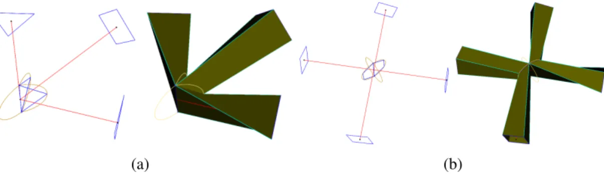
We call a scaffold regular if it has the same number of quads around each line segment. This is not an automatic property of standard scaffolds, as can be seen in figure 1.6b and 1.7.

5 edges 7 edges 6 edges 6 edges 6 edges 6 edges (a) (b) (c)

Figure 1.6: A three-fold rotation symmetry (C3). (a) Skeleton. (b) Standard scaffold. (c) Symmetric scaffold.

(a) (b) (c)

1.3. EXISTENCE OF SCAFFOLDS

To get regular scaffolds we need compatible cells that have the same number of points, this means that (1.3.3) must be replaced by

∑

f∈Ev

f((Sv∩e)

xv_f = λ ∀v ∈V_{Σ, e ( v, e ∈ EΣ} (1.3.15)

with λ an additional free variable. Notice that λ is independent of v ∈VΣand so (1.3.15) implies (1.3.3). Solutions to the linear system (1.3.15) satisfying (1.3.4) are called regular solutions. Regularity ensures that all segments have a similar cross profile: a polygon with λ sides. If there is a regular solution we say that (1.3.15) is feasible, which implies the existence of a regular scaffold.

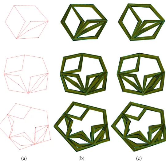
It is possible to get a scaffold that is at the same time regular and symmetric. We just need to ensure, besides (1.3.4), the extra constraints in (1.3.9). A regular scaffold need not be symmetric (Figure 1.8a). Conversely, a symmetric scaffold is not necessarily regular (Figure 1.8b).

Asymmetric cells

(a) (b)

Figure 1.8: Symmetry and regularity are independent properties. (a) Regular asymmetric scaffold: the highlighted cell is asymmetric with respect to the reflection symmetry. (b) Symmetric irregular scaffold: one edge has a quadrangular cross profile while the rest are pentagonal.

The existence of regular symmetric scaffolds is established in the following theorem. It is sufficient to prove the feasibility of regular symmetric scaffolds to automatically get the feasibility of regular scaffolds. Indeed a regular scaffold can be regarded as a regular symmetric scaffold withT_Σthe trivial group consisting of only the identity symmetry. Theorem 3. For any skeleton Σ admitting a group of symmetriesTΣ, the linear system given by (1.3.15) has a solution with the entries xv_f (v ∈V_Σ, f ∈ Ev) satisfying the constraints given in (1.3.4) and (1.3.9). Therefore there exists a regular symmetric scaffold for Σ.

Proof. As done in the proof of Theorem 1, for every v ∈V_Σ Lemma 1.3.1 gives a local solution( ˜xv_f, ˜λv) satisfying (1.3.1). Then ˆxv_f = s

ˆ λ ˜ λv˜ xv_{f with ˆλ = ∏u∈V} Σ ˜ λuand s = maxisi, is a local solution such that all the cells have s ˆλ points, thus ˆxv_f is a global solution

of (1.3.15) satisfying (1.3.4). Applying Lemma 1.3.2 to this solution we get a symmetric solution ¯xv_f with the same number of points on each cell. Indeed

| ¯C_ev| =

_∑

_∑

∑

∑

∑

_∑

Symmetry is an important property for the scaffolds as can be appreciated in Fig-ure 1.9 computed for one of the examples in [Karˇciauskas and Peters, 2016].

(a) (b)

Figure 1.9: With symmetric requirements a scaffold can be greatly improved. (a) The computation of the scaffold in Figure 1.1a without symmetric requirements. (b) The “correct” symmetric scaffold respecting all the symmetries of the skeleton (same as Figure 1.1a).

1.4

Optimal scaffolds

We have established that for any skeleton Σ admitting a group of symmetriesT_Σ, there exist a standard scaffold, a symmetric scaffold, a regular scaffold, and a regular symmetric scaffold. In this section we address the computation of optimal scaffolds. We model each scaffolding problem as an Integer Linear Program (IP) [Chen et al., 2009] that looks for a solution with a minimal number of quads. For this we need first to define an objective function, then the constraints of the IPs. The existence of a minimal solution is guaranteed by the existence theorems on Section 1.3, thus such minimal solutions can be computed with an IP solver.

1.4.1

Objective function

We want to express the total number of quads in a scaffold in terms of the subdivision of the arcs. For this we proceed as follows. LetQ be the set of all quads of a scaffold, and Pthe number of pairs hp, Qi such that p ∈ Q ∈Q. Then we have that

|Q| = 1

1.4. OPTIMAL SCAFFOLDS

Indeed, the last equation is a consequence of the following observation: every fixed quad Qhas 4 points and there are precisely 4 pairs hq, Qi with p ∈ Q.

We can count P in another way: by fixing first a point and then counting the pairs containing it. For a point p in the cell of a dangling node, there are 2 quads containing p. If p is a point in the cell of an articulation, there are 4 quads containing p. If p is a point in an arc on the boundary of a Voronoi region of a joint (not an articulation), we get that p is in 4 quads if p is not an extremity of the arc, or p is in 2d(p) quads if it is an extremity of an arc. Here d(p) denotes the number of Voronoi regions that have p in their common boundary.

The latter paragraph can be summarized as P=

_∑

_∑

_∑

where ΘΣis the number of pairs containing points that are extremities of the arcs in the Voronoi diagrams. Notice that ΘΣis a constant for a fixed skeleton Σ, thus (1.4.2) can be written as P=

_∑

_∑

_∑

where Φ_Σ= ΘΣ− ∑v∈N_Σ4|Ev| is a constant for a fixed skeleton Σ. From equations (1.4.1) and (1.4.3) we conclude that

∑

∑

_∑

∑

is an objective function that minimizes the total number of quads in a scaffold.

1.4.2

Integer Linear Programming models

We can now state the Integer Linear Programs (IPs) that compute subdivision for the arcs such that the scaffold have a minimal number of quads. For all the IPs the optimality criterion is to minimize the objective function (1.4.4). In Table 1.1 we show each model. Theorems 1, 2 and 3 prove the feasibility of the standard, symmetric, and regular symmetric models respectively. As discussed in Section 1.3.4, the feasibility of the regular IP model is a consequence of the feasibility of the regular symmetric model.

A final observation is that once we can guarantee feasibility, and since all the variables in (1.4.4) are positive integers, then an optimal minimal solution always exists. The optimal solution can be computed with a Mixed-Integer Linear Program Solver. In particular with the branch-and-cut [Chen et al., 2009, Chapter 12] implementation of GLPK [Makhorin, 2016].

Minimize Scaffold Constraints function Standard (1.3.3), (1.3.4) (1.4.4) Regular (1.3.15), (1.3.4) (1.4.4) Symmetric (1.3.3), (1.3.4), (1.3.9) (1.4.4) Regular Symmetric (1.3.15), (1.3.4), (1.3.9) (1.4.4)

Table 1.1: Integer Linear Program models.

1.5

Algorithms

In this section we provide practical algorithms for the implementation of our method. Although our main contribution is in the theoretical foundation and the proofs of the existence of scaffolds, the algorithms in this section show that our method can be readily implemented to compute scaffolds for any skeleton.

The general steps for an implementation are described in Algorithm 1. Sub-algorithms 2, 3 and 4 deal with the details of the construction of compatible cells from the output of the standard IP and the definition of the bijections between cells (linking process).

Input: The set of nodesVΣand edgesEΣrepresenting the skeleton. Output: The quads that represent a scaffold.

1 foreach node v ∈V_Σdo

2 Av← {e ∩ Sv: e ∈EΣ, e ( v}; 3 Hv← convexHull(Av); 4 Ev← edgesO f (Hv);

5 Define and solve the Linear Program for the subdivision of arcs; /* Alg. 2 */

6 Construct compatible cells; /* Alg. 3 */

7 Define bijections of linked cells; /* Alg. 4 */

8 foreach edge e = ab ∈E_Σdo 9 Let C_ea= hp0, p2, . . . , pni; 10 for i = 0 to n do

11 Output quad hpi, φe(pi), φe(pi+1), pi+1i /* i + 1 is taken mod n */

Algorithm 1: General algorithm for constructing a scaffold.

Algorithm 1 follows the general three steps we introduced in Section 1.1. In Step 1 we use spherical Voronoi diagrams for the partition of the sphere at the joints (lines 1–4). We mostly work with their duals, Delaunay triangulations, which are equivalent to the the convex hulls [Brown, 1979, Grima and Márquez, 2001]. The discretization of the regions, Step 2, is divided into sub-algorithms.

1.5. ALGORITHMS

The convex hull computed in Algorithm 1 (line 3) is not always 3-dimensional. It may be a 2-dimensional convex hull (a polygon), a 1-dimensional convex hull (one edge), or a 0-dimensional one (a point). Those cases correspond respectively to: more than three points in general position, more than two coplanar points, two points, and only one point (Figure 1.10). 1-dimensional convex hulls occur around articulations, while 0-dimensional ones are associated to dangling nodes. In our implementation the convex hull is computed by means of the QHull library [Barber et al., 1996].

(a) (b) (c) (d)

Figure 1.10: Cases for the convex hull ofAv. Edges of Evare shown in black. (a) 3-dimensional: more than three points in general position. (b) 2-dimensional: more than two coplanar points. (c) 1-dimensional: two points. (d) 0-dimensional: one point.

Algorithm 2 deals with the standard IP whose optimal solutions give compatible cells. It sets up and solves the IP using the convex hull representation of the regions. Simple modifications can be done for the other three variants of the scaffold. We follow (1.3.5). Thus we chose to have at least 4 points on each cell to guarantee at least quadrangular cross sections as in [Bærentzen et al., 2012, Ji et al., 2010, Panotopoulou et al., 2018, Usai et al., 2015, Yao et al., 2009]. We set the threshold for long arcs at 5π₆ (i.e δ =

π

6), above which at least two subdivisions must be done. In our implementation we solve the IP with the branch-and-cut [Chen et al., 2009, Chapter 12] implementation in GLPK [Makhorin, 2016].

Algorithm 3 computes the cells from the subdivision numbers and the convex hull representation of the Voronoi diagram, and such it must handle the different cases of the convex hulls (see Figure 1.10).

The heuristic for the linking process (Step 3) is described in Algorithm 4, from which the resulting quads are defined. It defines the bijections (links) by minimizing the total length of the links (same heuristic used in [Bærentzen et al., 2012]).

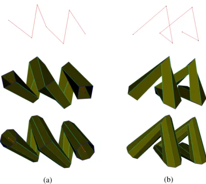
To better reflect the geometry of the model, and depending on the application at hand, the position of points in the discretization of each arc can be modified by a Laplacian smoothing [Botsch et al., 2010] or another heuristic. A global optimization could be further applied to take into account the twisting of the quads around a chain of articulation nodes (Figure 1.11). The challenge is in devising such a “better” positioning of points that also respects the symmetries of the skeleton. An intrinsic solution using our method is to subdivide each arc twice (or more) as shown in Figure 1.11.

Input: The set of nodesVΣand edgesEΣrepresenting the skeleton, along with Evfor each v ∈VΣ.

Output: The values xv_f representing the number of subdivisions for each arc that gives compatible cells.

1 Initialize the linear program IP;

2 foreach node v ∈V_Σ, and edge f∈ Evdo 3 Add integer variable xv_f to IP;

4 if the arc associated to xv_f has length<5π₆ εvthen 5 Add restriction xv_f ≥ 1 to IP;

6 else

7 Add restriction xv_f ≥ 2 to IP;

8 foreach pair (v, e) with v ∈V_Σ, e ∈E_Σand e( v do 9 Add following restriction to IP _∑

f∈Ev f((e∩Sv)

xv_f ≥ 4;

10 foreach edge e = ab ∈E_Σdo

11 Add following restriction to IP ∑ g∈Ea g((e∩Sv) xa_g= ∑ h∈Eb h((e∩Sv) xb_h;

12 _{Define objective function ∑v∈(VΣ−L}

Σ)∑f∈Ev2x v

f+ ∑v∈LΣ∑f∈Evx v

f for IP; 13 Solve IP by minimizing the objective function.

1.5. ALGORITHMS

Input: NodesVΣand edgesEΣof the skeleton, Ev,Hvand the subdivision numbers xv_f. Output: A listC of compatible cells for the scaffold.

1 C ← emptyList(); 2 foreach v ∈VΣdo

3 ifHvis 3-dimensionalthen

/* at least 4 not coplanar nodes */

4 foreach node ne inHvdo /* ne= e ∩ Sv for e( v */ 5 C_ev← emptyList();

6 foreach f ( (e ∩ Sv) do

7 Let F1, F2be the two faces inHvthat have common boundary f ; 8 Compute the outward pointing unit normals N₁, N₂of F₁, F₂

respectively;

9 Compute xv_f+ 1 points in the arc from v + N1to v + N2going perpendicularly to f on Sv;

10 Add the points to C_evavoiding repetitions; 11 Add C_evtoC ;

12 ifHvis 2-dimensionalthen

/* at least 3 nodes, all coplanar */

13 Let N₁, N₂be the two unit normals of the plane supportingHv;

14 foreach node ne inHvdo /* ne= e ∩ Sv for e( v */ 15 C_ev← emptyList();

16 Let f , g be the two edges incidents to ne;

17 Compute xv_f+ 1 points in the arc from v + N1to v + N2going perpendicularly to f on Sv;

18 Compute x_gv+ 1 points in the arc from v + N₁to v + N₂going perpendicularly to g on Sv;

19 Add the points to C_evavoiding repetitions; 20 Add C_evtoC ;

21 ifHvis 1-dimensionalthen

/* only one edge and 2 nodes */

22 Let f be the unique edge in Ev;

23 Compute xv_f points in the circle with center v and perpendicular to f on Sv; 24 Add the points to C_ev;

25 Add C_evtoC ;

26 ifHvis 0-dimensionalthen

/* only one node */

27 Compute xv_νv points in the great circle with center v and perpendicular to e on Sv; 28 Add the points to C_ev;

29 Add C_evtoC ; 30 returnC