HAL Id: hal-01962629
https://hal.inria.fr/hal-01962629
Submitted on 20 Dec 2018
HAL is a multi-disciplinary open access
archive for the deposit and dissemination of
sci-entific research documents, whether they are
pub-lished or not. The documents may come from
teaching and research institutions in France or
abroad, or from public or private research centers.
L’archive ouverte pluridisciplinaire HAL, est
destinée au dépôt et à la diffusion de documents
scientifiques de niveau recherche, publiés ou non,
émanant des établissements d’enseignement et de
recherche français ou étrangers, des laboratoires
publics ou privés.
Energy analysis of a solver stack for frequency-domain
electromagnetics
Emmanuel Agullo, Luc Giraud, Stéphane Lanteri, Gilles Marait, Anne-Cécile
Orgerie, Louis Poirel
To cite this version:
Emmanuel Agullo, Luc Giraud, Stéphane Lanteri, Gilles Marait, Anne-Cécile Orgerie, et al.. Energy
analysis of a solver stack for frequency-domain electromagnetics. [Research Report] RR-9240, Inria
Bordeaux Sud-Ouest. 2018. �hal-01962629�
ISSN 0249-6399 ISRN INRIA/RR--9240--FR+ENG
RESEARCH
REPORT
N° 9240
November 2018 Project-Team HiePACSEnergy analysis of a
solver stack for
frequency-domain
electromagnetics
Emmanuel Agullo, Luc Giraud, Stéphane Lanteri, Gilles Marait,
Anne-Cécile Orgerie, Louis Poirel
RESEARCH CENTRE BORDEAUX – SUD-OUEST
200 avenue de la Vielle Tour 33405 Talence Cedex
Energy analysis of a solver stack for
frequency-domain electromagnetics
Emmanuel Agullo
∗, Luc Giraud
∗, Stéphane Lanteri
∗,
Gilles Marait
∗, Anne-Cécile Orgerie
†, Louis Poirel
∗Project-Team HiePACS
Research Report n° 9240 — November 2018 — 15 pages
Abstract: High-performance computing (HPC) aims at developing models and simulations for applications in numerous scientific fields. Yet, the energy consumption of these HPC facilities currently limits their size and performance, and consequently the size of the tackled problems. The complexity of the HPC software stacks and their various optimizations makes it difficult to finely understand the energy consumption of scientific applications. To highlight this difficulty on a concrete use-case, we perform an energy and power analysis of a software stack for the simulation of frequency-domain electromagnetic wave propagation. This solver stack combines a high order finite element discretization framework of the system of three-dimensional frequency-domain Maxwell equations with an algebraic hybrid iterative-direct sparse linear solver. This analysis is conducted on the KNL-based PRACE-PCP system. Our results illustrate the difficulty in predicting how to trade energy and runtime.
Key-words: Energy consumption, HPC
∗Inria, France
Analyse énergétique d’une pile logicielle pour le calcul en
éléectromagnétisme
Résumé : Le calcul haute performance (HPC) vise à développer des modèles et des simulations dans de nombreux domaines scientifiques. Pourtant, la consommation d’énergie des installations de calcul haute performance limite actuellement leur taille et leur performance et, par conséquent, la taille des problèmes abordés. La complexité des piles logicielles de calcul haute performance et de leurs différentes optimisations rendent difficile la compréhension fine de la consommation énergétique des applications scientifiques. Pour mettre en évidence cette difficulté sur un cas d’utilisation concret, nous effectuons une analyse énergétique d’une pile logicielle pour des simulations de propagation d’ondes électromagnétiques dans le domaine fréquentiel. Ce solveur combine une approche de discrétisation par éléments finis d’ordre élevé pour le système d’équations de Maxwell tridimensionnelles dans le domaine fréquenciels et un solveur parallèle itératif hybride itératif-direct pour la résolution du système creux associé. Cette analyse est effectuée sur le Système PRACE-PCP à base de KNL. Nos résultats illustrent la difficulté à prédire un compromis en énergie et temps de calcul.
Energy Analysis of a Solver Stack 3
Contents
1 Introduction 4 2 Introduction 4 3 Numerical approach 5 4 Simulation software 5 5 MaPHyS algebraic solver 5 6 Numerical and performance result 6 6.1 Experimental setup . . . 6 6.2 MaPHyS used in standalone mode . . . 7 6.3 Scattering of a plane wave by a PEC sphere . . . 107 Conclusion 12
4 Agullo et al
1
Introduction
2
Introduction
The advent of numerical simulation as an essential scientific pillar has led to the co-development of hardware and software capable of solving larger and larger problems at a tremendous level of accuracy. The focus of performance-at-any-cost computer operations has led to the emergence of supercomputers that consume vast amounts of electrical power and produce so much heat that large cooling facilities must be constructed to ensure proper performance https://www.top500. org/green500. To address this trend, the Green500 list puts a premium on energy-efficient performance for sustainable supercomputing. In the meanwhile, the high-performance computing (HPC) community has faced the challenge with the emergence of energy-efficient computing. While many innovative algorithms [1, 2] have been proposed to reduce the energy consumption of the main kernels used in the numerical simulations, fewer studies [3] have tackled the overall energy analysis of a complex numerical software stack.
This work aims at conducting an energy and power analysis of the simulation of frequency-domain electromagnetic wave propagation, as detailed in Section 3. Such a simulation is represen-tative of a numerical simulation involving the usage of a complex software stack. In the present case, we study the combined HORSE/MaPHyS numerical software stack. The HORSE (High Order solver for Radar cross Section Evaluation) simulation software implements an innovative high order finite element type method for solving the system of three-dimensional frequency-domain Maxwell equations, as presented in Section 4. From the computational point of view, the central operation of a HORSE simulation is the solution of a large sparse and indefinite linear system of equations. High order approximation is particularly interesting for solving high frequency electromagnetic wave problems and, in that case, the size of this linear system can easily exceed several million unknowns. In this study, we adopt the MaPHyS [4] - [5] hybrid iterative-direct sparse system solver, which is based on domain decomposition principles [15]. MaPHyS is representative of fully-featured adaptive sparse linear solvers [14, 16, 8, 10] involving multiple numerical linear steps combining the usage of dense and sparse direct numerical linear algebra kernels as well as iterative methods, as further discussed in Section 5.
Energy consumption is a major concern putting a strain on HPC infrastructures’ budget [1]. Additionnaly, peak power consumption hampers the size of these infrastructures, challenging the electricity provisioning [2]. Power capping techniques have been developed to control this power consumption [11, 12]. While these techniques dynamically limit the power consumption of running nodes, we argue here that a better understanding of HPC applications behavior could be more beneficial in finding an adequate trade-off between performance, power and energy consumption. The objective of this paper is to study the energy profile of a complex software stack that is representative of numerical simulations. To perform the energy and power analysis, we rely on two tools, Bull Energy Optimizer (BEO) and High Definition Energy Efficiency Visualization (HDEEVIZ). We first study the behavior of the MaPHyS hybrid solver in a standalone fashion, showing the energy profiles of each of its numerical steps. We then study the behavior of the overall HORSE/MaPHyS simulation stack on a realistic 3D test case.
The rest of the paper is organized as follows. Section 3 briefly presents the high order discretization technique employed while Section 4 presents the HORSE simulation tool that implements it. Section 5 presents the MaPHyS sparse hybrid solver that is used to solve the underlying sparse linear system. Section 6 presents the methodology employed to conduct our energy analysis and discusses the energy profile of the considered software stack, before concluding in Section 7.
Energy Analysis of a Solver Stack 5
3
Numerical approach
During the last 10 years, discontinuous Galerkin (DG) methods have been extensively considered for obtaining an approximate solution of Maxwell’s equations. Thanks to the discontinuity of the approximation, this kind of methods has many advantages, such as adaptivity to complex geometries through the use of unstructured, possibly non-conforming, meshes, easily obtained high order accuracy, hp-adaptivity and natural parallelism. However, despite these advantages, DG methods have one main drawback particularly sensitive for stationary problems: the number of globally coupled degrees of freedom (DoF) is much larger than the number of DoF required by conforming finite element methods for the same accuracy. Consequently, DG methods are expensive in terms of both CPU time and memory consumption, especially for time-harmonic problems. Hybridization of DG (HDG) methods [13] is devoted to address this issue while keeping all the advantages of DG methods. HDG methods introduce an additional hybrid variable on the faces of the elements, on which the definition of the local (element-wise) solutions is based. A so-called conservativity condition is imposed on the numerical trace, whose definition involves the hybrid variable, at the interface between neighbouring elements. As a result, HDG methods produce a linear system in terms of the DoF of the additional hybrid variable only. In this way, the number of globally coupled DoF is reduced. The local values of the electromagnetic fields can be obtained by solving local problems element-by-element. We have recently designed such a high order HDG method for the system of 3D time-harmonic Maxwell’s equations [13].
4
Simulation software
HORSE is a computational electromagnetic simulation software for the evaluation of radar cross section (RCS) of complex structures. This software aims at solving the full set of 3D time-harmonic Maxwell equations modeling the propagation of a high frequency electromagnetic wave in interaction with irregularly shaped structures and complex media. It relies on an arbitrary high order HDG method that is an extension of the method proposed in [13]. This HDG method designed on an unstructured possibly non-conforming tetrahedral mesh, leads to the formulation of an unstructured complex coefficient sparse system of linear equations for the DoF of the hybrid variable, while the DoF of the components of the electric and magnetic fields are computed element-wise from those of the hybrid variable. This software is written in Fortran 95. It is parallelized for distributed memory architectures using a classical SPMD strategy combining a partitioning of the underlying mesh with a message-passing programming model using the MPI standard. One important computational kernel of this software is the solution of a large sparse linear system of complex coefficients equations. In a preliminary version of this software, this system was solved using parallel sparse direct solvers such as MUMPS [7] or PaStiX [9]. However, sparse direct solvers may have a limited scalability when it comes to solve very large linear systems arising from the discretization of large 3D problems. In this paper, we instead rely on a hybrid iterative/direct solver. We employ the MaPHyS solver, discussed below, to do so.
5
MaPHyS algebraic solver
The solution of large sparse linear systems is a critical operation for many academic or industrial numerical simulations. To cope with the hierarchical design of modern supercomputers, hybrid solvers based on algebraic domain decomposition methods have been proposed, such as PDSLin [14], ShyLU [16], HIPS [8] or HPDDM [10]. Among them, approaches consisting of solving the problem on the interior of the domains with a sparse direct method and the problem on their
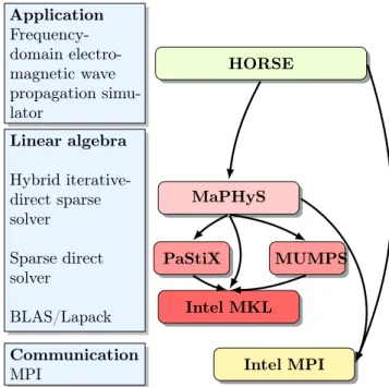
6 Agullo et al Application Frequency-domain electro-magnetic wave propagation simu-lator Linear algebra Hybrid iterative-direct sparse solver Sparse direct solver BLAS/Lapack Communication MPI HORSE MaPHyS PaStiX MUMPS Intel MKL Intel MPI
Figure 1: Software architecture of the solver stack.
interface with a preconditioned iterative method applied to the related Schur Complement have shown an attractive potential as they can combine the robustness of direct methods and the low memory footprint of iterative methods.
MaPHyS (Massively Parallel Hybrid Solver) [4] - [5] is a parallel linear solver, which implements this idea. The underlying idea is to apply to general unstructured linear systems domain decomposition ideas developed for the solution of linear systems arising from PDEs. The interface problem, associated with the so-called Schur complement system, is solved using a block preconditioner with overlap between the blocks that is referred to as Algebraic Additive Schwarz. Although MaPHyS has the functionality of exploiting two level parallelism using threads within an MPI process, this feature was not used in this study and focus was made on flat MPI performance only. MaPHyS makes use of a sparse direct solver as a subdomain solver such as MUMPS or PaStiX. The parallelization of the direct solver relies on a specific partitioning of the matrix blocks. PaStiX and MUMPS make extensive use of highly optimized dense linear algebra kernels (e.g., BLAS kernels).
A representation of the software architecture is given in Figure 1.
6
Numerical and performance result
6.1
Experimental setup
For the numerical simulations reported below we have used the PaRtnership for Advanced Computing in Europe - Pre-Commercial Procurement (PRACE-PCP) Intel “Manycore” Knights Landing (KNL) cluster Frioul at GENCI-CINES. Each node is a KNL 7250 running at 1.4GHz with 68 cores and up to 4 threads per core (272 threads per node) with 16 GB of MCDRAM and 192 GB of RAM.
The MaPHyS solver is used in version 0.9.6. PaStiX 6.0 is employed internally for processing
Energy Analysis of a Solver Stack 7
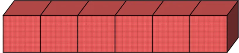
Figure 2: 2.5D test case with 6 subdomains along a 1D decomposition, used for the standalone MaPHyS experiments.
subdomains (see "sparse direct step" below) and MUMPS 5.0.2 is used for processing the coarse space for the dense+CSC variant (see "dense+CSC" below). We rely on Intel MKL 2017.0.0 for achieving high performance BLAS and LAPACK. In particular, the Intel MKL DSYGVX routine is used for computing the eigenvalue problem in the subdomains in the case of the dense+CSC variant (see "dense+CSC" below).
The energy measurements are performed with two tools developed by Atos-Bull: BEO v1.0 and HDEEVIZ. The former has been used to obtain accurate measures of the total energy spent for the MaPHyS computation; the latter to visualize with a fine time resolution the variations of the energy consumption during the execution.
6.2
MaPHyS used in standalone mode
The weak scalability of the MaPHyS solver is first investigated in a standalone mode. For these experiments, we solve a 3D Poisson problem on a 2.5D domain that corresponds to a beam and a 1D decomposition, as shown in Figure 2. Each subdomain has at most two neighbors and is essentially a regular cube of size 403 (i.e., each subdomain has approximately 64,000 unknowns).
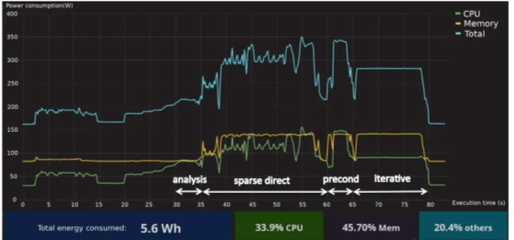
The energy performance has been measured with BEO as the total energy consumed by the job. We have also used the Bull HDEEVIZ graphic tool for a detailed visualization of the energy consumption over time. In Figure 5, we display the energy profile provided by this tool on a typical run of MaPHyS. The main steps of the hybrid solver can be observed by matching the execution time given by HDEEVIZ with the MaPHyS output timers. Thus we can identify these four steps:
• analysis: corresponds to the initialization of MaPHyS, reading the subdomain from dumped files and performing some preliminary index computations and communications;
• sparse direct: corresponds to the factorization of the local matrix associated with internal unknowns and the computation of the Schur complement associated with the interface unknowns;
• precond: the preconditioning step consists of the computation of the local preconditioner and involves neighbor to neighbor communications plus the factorization of the assembled local Schur complement. This factorization might be either dense or sparse depending on the preconditioning strategy further described below;
• iterative: the iterative step aims at computing the solution of the Schur complement system using a preconditioned Krylov subspace method; that is the Conjugate Gradient for the Poisson problem or GMRES for the electromagnetic computation.
The local matrices are read from files, which is both time and energy consuming but not really relevant to MaPHyS performance, since the matrices are usually computed locally and directly
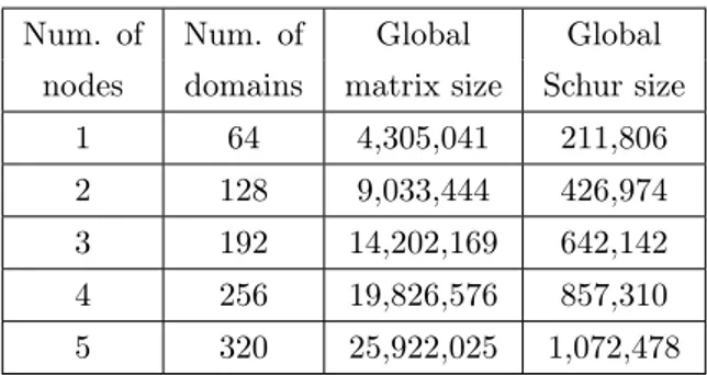
8 Agullo et al Num. of Num. of Global Global
nodes domains matrix size Schur size 1 64 4,305,041 211,806 2 128 9,033,444 426,974 3 192 14,202,169 642,142 4 256 19,826,576 857,310 5 320 25,922,025 1,072,478
Table 1: Main characteristics of the numerical example considered in the standalone MaPHyS experiments.
provided to the solver by the application codes such as HORSE for the experiments reported in the next section. This file access appears on the profile before the analysis starts.
We have considered five test cases whose properties are displayed in Table 1 and assessed three numerical variants of the solver that are referred to as:
• dense: we consider the fully assembled local Schur complements to build the additive Schwarz preconditioner; only dense linear algebra kernels, cpu intensive with very regular memory access patterns, are then used in the preconditioner application at each iteration of the iterative step.
• sparse: the entries of the local dense Schur complements that are smaller than a given relative threshold (10−5) are discarded; the resulting sparse matrices are then used to
build the additive Schwarz preconditioner; mostly sparse linear algebra kernels, less cpu demanding with very irregular memory access patterns, are then used when applying the preconditioner in the iterative part.
• dense+CSC: in addition to the previously described dense preconditioner, a coarse space correction [6] (CSC) is applied to ensure that the convergence will be independent from the number of subdomains. In this experiment we compute five vectors per subdomain to create the coarse space. The coarse space being relatively small compared to the global problem, computations are centralized onto one process and solved by the direct solver (MUMPS in the experiments reported here).
As it can be seen in Figure 5 (power profile of the dense variant on a single node execution), the memory energy consumption represents a significant part of the total (45.7%), which is consistent with the current trend: floating point operations are cheap while memory accesses are relatively costly. One can furthermore observe that the setup and analysis parts of the run have a low energy consumption. The three numerical steps of the MaPHyS solver can be clearly identified through the combined observation of the memory and CPU power profiles. The iterative solve step appears quite clearly as a large plateau, where the power consumption is high for memory and low for CPU. It is consistent with the fact that this step is memory bound with many communications and relatively few computations. The total energy consumed by the node is 5.6 Wh = 20,160 J, which corresponds to the results given by BEO for this case.
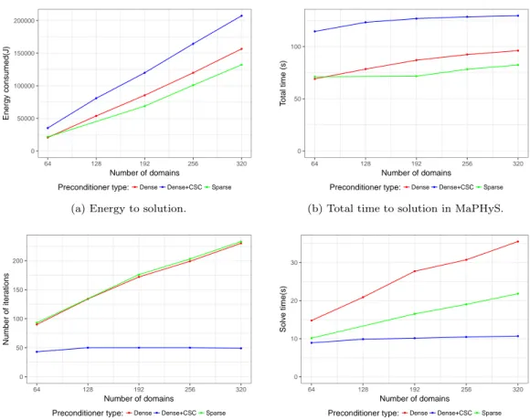
We also report the total energy of the job provided by BEO, the total time to solution, the number of iterations and the time spent in the iterative step, in figures 4a, 4b, 4c and 4d, respectively. The time of each step of the solver is represented Figure 3. A value is missing for the “sparse” curve with 128 subdomains due to measurement error.
Energy Analysis of a Solver Stack 9
Dense Dense+CSC Sparse
64 128 192 256 320 64 128 192 256 320 64 128 192 256 320 0 50 100 Number of domains Time (s)
Solver step: Analysis Schur Factorization Pcd Setup Iterative Solve
Figure 3: Step by step time performance for MaPHyS.
● ● ● ● ● ● ● ● ● ● ● ● ● ● 0 50000 100000 150000 200000 64 128 192 256 320 Number of domains Energy consumed(J)
Preconditioner type: ●Dense●Dense+CSC●Sparse
(a) Energy to solution.
● ● ● ● ● ● ● ● ● ● ● ● ● ● 0 50 100 64 128 192 256 320 Number of domains T otal time (s)
Preconditioner type: ●Dense●Dense+CSC●Sparse
(b) Total time to solution in MaPHyS.
● ● ● ● ● ● ● ● ● ● ● ● ● ● 0 50 100 150 200 64 128 192 256 320 Number of domains Number of iter ations
Preconditioner type: ●Dense●Dense+CSC●Sparse
(c) Number of iterations. ● ● ● ● ● ● ● ● ● ● ● ● ● ● 0 10 20 30 64 128 192 256 320 Number of domains Solv e time(s)
Preconditioner type:●Dense●Dense+CSC●Sparse
(d) Time in the iterative step of MaPHyS.
Figure 4: Time and energy performance for MaPHyS .
We observe that, despite the extra-memory traffic due to indirections, the fact that it induces much fewer floating point operations than the dense variant leads to a lower overall energy consumption. The high energy required by the dense+CSC preconditioner is mainly due to the
10 Agullo et al
Figure 5: Power dissipation over the execution time of MaPHyS, visualized with HDEEVIZ. setup of the CSC, which is both memory and CPU demanding. Because the dense and sparse preconditioners do not implement any global coupling numerical mechanisms, the number of iterations is expected to grow as the number of subdomains for the 1D decomposition of the domain on the Poisson test example. This poor numerical behavior can be observed in Figure 4c, while it can be seen that the coarse space correction (dense+CSC variant) plays its role and ensures a number of iterations independent from the number of domains (see [6] for further insights on the numerical properties of the method). This nice numerical behavior translates in terms of time to solution for the iterative part where the dense+CSC method outperforms the two other variants. However, the overhead of the setup phase for the construction of the coarse space, which requires the solution of generalized eigenproblems, is very high and cannot be amortized at that intermediate scale if only a single right-hand side has to be solved (which would not be the case for, e.g., radar cross section evaluation as considered in Section 6.3, where multiple right-hand sides must be solved in real-life test cases). Nonetheless, the relative ranking in terms of power requirements are different. Through a simple linear regression, we can observe that the average power requirements are about 328, 326 and 321 W/node for the dense, sparse and dense+CSC preconditioners, respectively.
6.3
Scattering of a plane wave by a PEC sphere
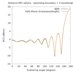
We now consider a more realistic problem that consists in the scattering of a plane wave with a frequency F=600 MHz by a perfectly electric conducting (PEC) sphere. The contour lines of the x-component of the electric field are displayed in Figure 6a, and the obtained RCS is plotted in Figure 6b together with a comparison with a reference RCS obtained from a highly accurate (but costly) BEM (Boundary Element Method) calculation. This problem is simulated using the coupled HORSE/MaPHyS numerical tool. The underlying tetrahedral mesh contains 37,198 vertices and 119,244 elements. We have conducted a series of calculations for which the number of iterations of the MaPHyS interface solver has been fixed to 100. Simulations are performed using a flat MPI mode, binding one MPI process per physical core without any shared memory parallelism. We consider the following two situations: (a) the interpolation order in the HDG discretization method is uniform across the cells of the mesh; (b) the interpolation order is adapted locally to the size of the cell based on goal-oriented criterion. In the latter situation, we distribute the interpolation order such that there are at least 9 integration points (degrees of freedom of the Lagrange basis functions) per local wavelength. For the particular tetrahedral
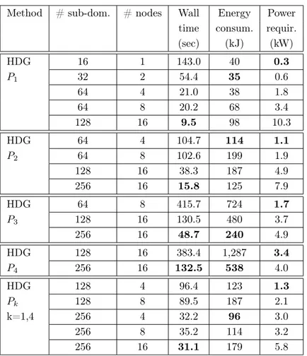
Energy Analysis of a Solver Stack 11 Method # sub-dom. # nodes Wall Energy Power
time consum. requir. (sec) (kJ) (kW) HDG 16 1 143.0 40 0.3 P1 32 2 54.4 35 0.6 64 4 21.0 38 1.8 64 8 20.2 68 3.4 128 16 9.5 98 10.3 HDG 64 4 104.7 114 1.1 P2 64 8 102.6 199 1.9 128 16 38.3 187 4.9 256 16 15.8 125 7.9 HDG 64 8 415.7 724 1.7 P3 128 16 130.5 480 3.7 256 16 48.7 240 4.9 HDG 128 16 383.4 1,287 3.4 P4 256 16 132.5 538 4.0 HDG 128 4 96.4 123 1.3 Pk 128 8 89.5 187 2.1 k=1,4 256 4 32.2 96 3.0 256 8 35.2 114 3.2 256 16 31.1 179 5.8
Table 2: Performance of the coupled HORSE/MaPHyS software stack. Scattering of a plane wave by a PEC sphere. Timings for 100 iterations of the interface solver of MaPHyS.
mesh used in this study, we obtain the following distribution of polynomial approximation within the mesh elements: 12,920 P1 elements, 70,023 P2 elements, 31,943 P3 elements and 4,358 P4
elements. For a given mesh, a uniform interpolation order is not necessarily the best choice in terms of computational cost versus accuracy, especially if the mesh is unstructured as it is the case here. Increasing the interpolation order allows for a better accuracy at the expense of a larger sparse linear system to be solved by MaPHyS. Distributing the interpolation order according to the size of the mesh cells allows for a good trade-off between time to solution and accuracy.
The performance in terms of both time and energy consumption are reported in Table 2. In this table, the number of subdomains also corresponds to the total number of core or MPI processes. The number of MPI processes per node can be deduced from the number of nodes. First of all, in most of the tested configurations, we observe a superlinear speedup, as a result of the reduction of the size of the local discretization matrices within each subdomain. The size n of the local matrices roughly decreases linearly with the number of domains but the arithmetic complexity for their factorization is O(n2) that leads to this superlinear effect. We first note, as
expected, that the energy consumption with higher values of the interpolation order increases, since the size of the HDG sparse linear system increases drastically. For a given number of subdomains, a second noticeable remark is that the energy consumption increases when the
12 Agullo et al
(a) Contour lines of the x-component of the electric field.
(b) Contour lines of the x-component of the RCS.
Figure 6: Scattering of a plane wave by a perfectly electric conducting sphere.
number of MPI processes per node decreases; this leads to a higher network traffic and moving data through the network is more costly than moving them in memory. For instance, for the HDG-P1 method, Using a decomposition of the tetrahedral mesh in 64 subdomains, the energy
consumption is equal to 38 kJ on 4 nodes (i.e., with 16 MPI processes per node) and 68 kJ on 8 nodes (i.e., with 8 MPI processes per node). A similar behavior is observed for the HDG-P2
method and a 64 subdomain decomposition.
The power consumption increases with the number of nodes due to their idle power consumption (i.e. power consumption when being switched one but performing no useful task). Yet, this characteristic does not order the energy consumption. Indeed, for the HDG-P1 method, the
energy consumption is higher with 1 node than with 2 or 4 nodes, but lower than with 8 or 16 nodes. This situation highlights the fact that the most energy-efficient solution is not always the faster time-to-solution or the least number of nodes: the trade-off lies in-between these two performance metrics and is specific to the considered solving method.
A final comment is that the use of a locally adapted distribution of the interpolation order allows for a substantial reduction of the energy consumption for a target accuracy. This is in fact the result of lowering the computing time solution because of the reduction of the size of the problem, as it can be seen by comparing the figures for the HDG-P4 and HDG-Pk methods
with a 256 subdomain decomposition. Finally, for a given test example, the best computing time does not correspond to the best energy to solution; the policies to determine the best trade-off between these two criteria will be the subject of future work.
7
Conclusion
Through the experiments conducted within this work, several lessons have been learnt on the numerical software designer side. For the numerical linear algebra solvers, we have seen that the best time to solution solver is also the best in terms of energy to solution, but not necessarily in terms of power requirement. From the application perspective, we have observed that the local polynomial order adaptivity, i.e., HDG-Pk not only provides the best trade-off in terms of
amount of memory and number of floating point operations, but also a nice trade-off in terms of
Energy Analysis of a Solver Stack 13 energy consumption. As for the linear solver, the best option in terms of energy might not be the best one in terms of power.
Acknowledgment
This work was partially financially supported by the PRACE project funded in part by the EU’s Horizon 2020 research and innovation programme (2014-2020) under grant agreement 653838.
14 Agullo et al
References
[1] Balaprakash, P., Tiwari, A., and Wild, S. M. (2014). Multi Objective Optimization of HPC Kernels for Performance, Power, and Energy. In Jarvis, S. A., Wright, S. A., and Hammond, S. D., editors, High Performance Computing Systems. Performance Modeling, Benchmarking and Simulation, pages 239–260. Springer International Publishing.
[2] Gholkar, N., Mueller, F., Rountree, B., and Marathe, A. (2018). PShifter: Feedback-based Dynamic Power Shifting Within HPC Jobs for Performance. In International Symposium on High-Performance Parallel and Distributed Computing (HPDC), pages 106–117.
[3] Li, B., Chang, H., Song, S., Su, C., Meyer, T., Mooring, J., and Cameron, K. W. (2014a). The Power-Performance Tradeoffs of the Intel Xeon Phi on HPC Applications. In IEEE International Parallel Distributed Processing Symposium Workshops, pages 1448–1456. [4] Giraud, L., Haidar, A., and Watson, L. T. (2008). Parallel scalability study of hybrid
preconditioners in three dimensions. Parallel Computing, 34:363–379.
[5] Agullo, E., Giraud, L., Guermouche, A., and Roman, J. (2011). Parallel hierarchical hybrid linear solvers for emerging computing platforms. Compte Rendu de l’Académie des Sciences - Mécanique, 339(2-3):96–105.
[6] Agullo, E., Giraud, L., and Poirel, L. (2016). Robust coarse spaces for Abstract Schwarz preconditioners via generalized eigenproblems. Research Report RR-8978, INRIA Bordeaux. [7] Amestoy, P. R., Duff, I. S., and L’Excellent, J.-Y. (2000). Multifrontal parallel distributed symmetric and unsymmetric solvers. Computer Methods in Applied Mechanics and Engi-neering, pages 501–520.
[8] Gaidamour, J. and Hénon, P. (2008). A parallel direct/iterative solver based on a Schur complement approach. 2013 IEEE 16th International Conference on Computational Science and Engineering, 0:98–105.
[9] Hénon, P., Ramet, P., and Roman, J. (2002). PaStiX: A High-Performance Parallel Direct Solver for Sparse Symmetric Definite Systems. Parallel Computing, 28(2):301–321.
[10] Jolivet, P., Hecht, F., Nataf, F., and Prud’homme, C. (2013). Scalable Domain Decomposition Preconditioners for Heterogeneous Elliptic Problems. In Proceedings of the International Conference on High Performance Computing, Networking, Storage and Analysis, SC ’13, pages 80:1–80:11, New York, NY, USA. ACM.
[11] Kelley, J., Stewart, C., Tiwari, D., and Gupta, S. (2016). Adaptive Power Profiling for Many-Core HPC Architectures. In IEEE International Conference on Autonomic Computing (ICAC), pages 179–188.
[12] Khan, K. N., Hirki, M., Niemi, T., Nurminen, J. K., and Ou, Z. (2018). RAPL in Action: Experiences in Using RAPL for Power Measurements. ACM Trans. Model. Perform. Eval. Comput. Syst., 3(2):9:1–9:26.
[13] Li, L., Lanteri, S., and Perrussel, R. (2014b). A hybridizable discontinuous Galerkin method combined to a Schwarz algorithm for the solution of 3d time-harmonic Maxwell’s equations. Journal of Computational Physics, 256:563–581.
Energy Analysis of a Solver Stack 15 [14] Li, X. S., Shao, M., Yamazaki, I., and Ng, E. G. (2009). Factorization-based sparse solvers
and preconditioners. Journal of Physics: Conference Series, 180(1):012015.
[15] Mathew, T. P. A. (2008). Domain Decomposition Methods for the Numerical Solution of Partial Differential Equations, volume 61. Springer Science & Business Media.
[16] Rajamanickam, S., Boman, E. G., and Heroux, M. A. (2012). ShyLU: A hybrid-hybrid solver for multicore platforms. Parallel and Distributed Processing Symposium, International, 0:631–643.
RESEARCH CENTRE BORDEAUX – SUD-OUEST
200 avenue de la Vielle Tour 33405 Talence Cedex
Publisher Inria
Domaine de Voluceau - Rocquencourt BP 105 - 78153 Le Chesnay Cedex inria.fr