Monetary Policy, Oil Stabilization Fund and the Dutch Disease

HAL Id: hal-01796312

https://hal.archives-ouvertes.fr/hal-01796312

Preprint submitted on 19 May 2018

HAL is a multi-disciplinary open access

archive for the deposit and dissemination of sci-entific research documents, whether they are pub-lished or not. The documents may come from teaching and research institutions in France or

L’archive ouverte pluridisciplinaire HAL, est destinée au dépôt et à la diffusion de documents scientifiques de niveau recherche, publiés ou non, émanant des établissements d’enseignement et de recherche français ou étrangers, des laboratoires

Monetary Policy, Oil Stabilization Fund and the Dutch

Disease

Jean-Pierre Allegret, Mohamed Benkhodja, Tovonony Razafindrabe

To cite this version:

Jean-Pierre Allegret, Mohamed Benkhodja, Tovonony Razafindrabe. Monetary Policy, Oil Stabiliza-tion Fund and the Dutch Disease. 2018. �hal-01796312�

Monetary Policy, oil Stabilization

Fund and the dutch diSeaSe

Documents de travail GREDEG

GREDEG Working Papers Series

Jean-Pierre Allegret

Mohamed Tahar Benkhodja

Tovonony Razafindrabe

GREDEG WP No. 2018-06

Les opinions exprimées dans la série des Documents de travail GREDEG sont celles des auteurs et ne reflèlent pas nécessairement celles de l’institution. Les documents n’ont pas été soumis à un rapport formel et sont donc inclus dans cette série pour obtenir des commentaires et encourager la discussion. Les droits sur les documents appartiennent aux auteurs.

Monetary Policy, Oil Stabilization Fund

and the Dutch Disease

Jean-Pierre Allegret

Mohamed Tahar Benkhodja

Tovonony Raza…ndrabe

GREDEG Working Paper No. 2018-06

Abstract

This paper contributes to the literature on the Dutch disease e¤et in a small open oil exporting economy. Speci…cally, our contribution to the liter-ature is twofold. On the one hand, we formulate a DSGE model in line with the balanced-growth path theory. On the other hand, besides alternative monetary rules, the model introduces an oil stabilization fund, an oil price rule, and a …scal rule. Our aim is to analyze to what extent the combina-tions between our alternative monetary rules and …scal policy are e¤ective to prevent a Dutch disease e¤ect in the aftermath of a positive oil price shock. Our main …ndings show that the Dutch disease, through the spending e¤ect, occurs only in the case of in‡ation targeting regime. An expansionary …scal policy contributes to improve the state of the economy through its impact on the productivity of the manufacturing sector.

Keywords: Monetary Policy, Oil Stabilization Fund, Dutch disease, Oil Prices, DSGE model.

JEL Classi…cation: E52, F41, Q40

Université Côte d’Azur, CNRS, GREDEG, France

y_{ESSCA, School of Management} z_{CREM, Université Rennes 1}

1

Introduction

For a long time, oil price ‡uctuations have always been at the center of macro-economic analysis. Several studies have been undertaken to understand the conse-quences of this shock on economic activity. Much of the existing literature has been devoted to the examination of the monetary policy reaction to oil price shocks, es-pecially in industrialized economies. Some others, examined the role of …scal policy. This paper analyzes the role of monetary and …scal policies in an oil exporting economy to see to what extent in the aftermath of a positive oil price shock, the deindustrialisation phenomenon, as de…ned in the Dutch disease literature, occurs. In order to analyse this e¤ect, we build a small open oil exporting model using a multi-sectoral medium-scale DSGE framework as in Christo¤el et al 2008 and

Stahler and Thomas 2012. We assume that the central bank sets the short-term nominal interest rate following an extended Taylor rule and accumulates foreign exchange reserves. We assume that the central bank adopts alternative monetary policy rules, namely a strict in‡ation targeting, a …xed exchange rate regime and a domestic oil price in‡ation as in Frankel (2011, 2017). We also assume that the government subsidy the price of domestically consumed re…ned oil as a combination of the current world price expressed in local currency and the last period’s domestic price. Also, the government holds an oil stabilization fund and accumulates foreign exchange reserves. Importantly, this paper di¤ers from previous papers by combining di¤erent monetary rules with …scal policy to assess their e¤ectiveness to face Dutch disease e¤ect.

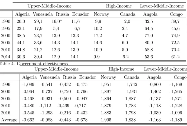
An extensive literature on oil exporting countries tends to focus either on high-income economiesLama and Medina, 2012 or low-income and lower-middle-income economies (IMF, 2012; Berg et al., 2013). A second signi…cant di¤erence from previous papers in that we analyze upper-middle-income oil exporters. More specif-ically, within this group, we consider oil-exporters sharing characteristics that bring them closer to lower-middle-income economies, i.e. Algeria and Venezuela. Appen-dix 1 exhibits several indicators stressing this important feature. Relative to other upper-middle-income and high-income oil-exporters, their experience a higher oil dependence as in lower-income economies. This oil dependence is observed both in terms of oil exports in total exports (Table 2) and oil exports as a share of GDP

(Table 3). Table 4 reveals another important fact for our purpose: government e¤ectiveness in oil-exporters such as Algeria and Venezuela is relatively weak. Gov-ernment e¤ectiveness refers, among others, to institutional e¤ectiveness, quality of infrastructure and public administration. In other words, the question of public investment e¢ ciency (Berg et al., 2013) is especially sensitive in these countries.

Our main …ndings show that the Dutch disease occurs only under in‡ation tar-geting and oil price in‡ation rules. The …xed exchange rate monetary rule seems to be e¤ective to prevent a Dutch disease e¤ect. Also, under IT rule, the decline in export sector tends to shrink gradually as the rise in the share of OSF dedicated to the support export sector. The decline in export goods production is completely resorbed when we combine the share of oil stabilisation fund (OSF hereafter) with a positive coe¢ cient of enhancing productivity. This is not the case when oil price in‡ation rule is considered. Finally, optimal monetary and …scal policies do not give better results than ER rule which also gives the highest welfare gain.

The remainder of the paper is organized as follows. Section 2, presents the review of the literature dedicated to the Dutch disease e¤ect that is modeled using DSGE models. Section 3, describes the model. Section 4, discusses the parameters calibration. Section 5 exposes the main results. Section 6 presents the conclusion.

2

Literature review

Our paper is related to three strands of the literature using dynamic stochastic general equilibrium (DSGE) models. This …rst one is the literature dedicated to the Dutch disease e¤ect. Acosta et al. (2009) investigate the e¤ects of remittances on resource reallocation and the real exchange rate. They show that sizeable remit-tances are associated to real exchange appreciation, which in turn, lead to a decline in the production of tradable goods. Cherif (2013)suggests that Dutch disease tends to be more severe in developing countries. The model includes two externalities -the presence of learning-by-doing in the tradable sector and cross-country knowledge spillovers. The spending e¤ect tends to be stronger in developing countries insofar as the increase in income in terms of domestic wages in the aftermath of the foreign transfer is greater than in economies with lower technological gap. Alberola and Benigno (2017)consider an additional channel through the degree of …nancial

open-ness of the economy. Financial openopen-ness ampli…es the domestic impacts of a positive shock on commodity price. More speci…cally, commodity exporters experience an improvement in their net foreign asset position. This positive wealth e¤ect increases domestic demand leading to a permanent reallocation of resources from the tradable sector to the non-tradable one.

A second strand of literature focuses on resource-rich low-income countriesIMF (2012). Berg et al. (2013)contribute to the debates on the management of revenues from nonrenewable resources in low-income countries. They advocate a “sustainable investing approach” combining a rise in public investment -to respond to capital-scarcity- and saving a part of the resources in a fund -to face both recurrent costs for operation and maintenance and resource exhaustion. The model has some in-teresting distinguishing features for our purpose. First, the Dutch disease e¤ect is captured through a learning-by-doing externality in the traded sector. Second, public investment exerts an in‡uence on the productivity in both the nontraded and traded good sectors. In other words, the government can implement an in-vestment strategy to counterbalance the Dutch disease phenomenon resulting from a positive commodity shock. Third, public investment su¤ers from two important distortions: a low public investment e¢ ciency on the one hand; absorptive capacity constraints in the economy in the other hand. In a relatively close perspective,Alter et al. (2017) investigate the public investment strategy in a context of natural re-source depletion.The model includes institutional failures through project selection weakness. As Berg et al. (2013), they conclude in favor of a scaling-up investment strategy in which the government increases its investment in the economy promot-ing the diversi…cation of the economy and the development of infrastructures while simultaneously taking into account the need to ensure …scal stability over time.

The third strand of literature focuses on macroeconomic stabilization policy in the aftermath of oil price shocks. On the monetary policy side, Lama and Medina (2012)study the role of an exchange rate stabilization policy to face Dutch disease e¤ect. Their model includes a real rigidity under the form of learning-by-doing ex-ternalities in the tradable sector. They …nd that exchange rate stabilization policy may prevent the real appreciation of the domestic currency, and hence a fall in the tradable production, but this policy may increase macroeconomic volatility to the

stabilization policy is welfare-reducing relative to a ‡oating regime. Dagher et al. (2012) analyze the short-run e¤ects of oil windfalls in low-income countries. They assume the presence of bottlenecks in the economy and non-optimizing households. An important …nding is the counterproductive e¤ect of reserve accumulation in re-sponse to a positive oil shock as this strategy crowds out both private consumption and investment. Dagher et al. (2012)suggest that the best response is the coordi-nation of reserve accumulation policy with the …scal policy where reserves are saved externally in a sovereign wealth fund. Faltermeir et al. (2017) investigate whether the accumulation of foreign exchange reserves is welfare-improving in countries suf-fered from a Dutch disease e¤ect. In an economy exhibiting nominal rigidities and learning-by-doing externalities in the tradable sector, they …nd that large and sus-tained accumulation of reserves is welfare-improving insofar as this strategy allows higher gains relative to a peg regime or a policy rate rule. On the …scal side, an extensive literature has been dedicated to …scal rules as public spending tend to go hand in hand with oil receipts, generating pro-cyclical policy (Baunsgaard et al., 2012; El Anshasy and Bradley, 2012). Arezki and Ismail (2013)investigate the behavior of the real exchange rate during the boom-bust commodity price cycle. While the real exchange rate appreciates during the boom phase, the depreciation is smaller than the fall of commodity price during the bust period. This disconnection is due to the …scal policy adopted by governments in rich-resource countries.The lack of …scal discipline implies a bias in …scal spending -due to political pressures- during the boom-bust cycle. As current spending exhibits a high domestic content, this bias tends to exert a structural pressure on non-tradable good prices, and, hence, on the real exchange rate appreciation. Fiscal smoothing plays a critical role to manage both short- and medium-term e¤ects of a commodity windfall. Pieschacón (2012) -by comparing Mexican and Norwegian experiences- highlights the welfare improving of …scal rules that insulate the domestic economy from oil price shocks.

3

The Model

In line with the balanced-growth path theory, we assume that real variables will share the same evolution as the labor-augmenting technology process t. Therefore,

by the consumer price level Pt. Tranformed variables are represented by lower-case

letters which in the literature is known as "intensive form" representation. For instance, ct = Ct= t and pH;t = PH;t=Pt represent respectively the stationary level

of consumption and relative price of domestic goods.1 _{It is important to note that}

the level of hours worked Lt is already stationary and no further transformation is

needed. The growth rate of the labor-augmenting technology process g ;t = t= t 1

is assumed to evolve according to:

ln(g ;t) = (1 g ) ln(g ) + g ln(g ;t 1) + gt

where g_t iid N 0; 2

g and g is the steady-state value of g ;t. For the sake

of clarity, the following presentation of the model does not include productivity di¤erential between home and foreign countries, price and wage dispersion across …rms and households, and adjustment cost when changing the level of imported goods in the …nal-good production process.2

3.1

Households

The population size in the oil-exporting country is normalized to unity, h = [0; 1]. Representative household within the oil-exporting (Home) country maximizes a string of discounted future value of utilities given by:

Et 1 X k=0 k_U t+k(ct+k(h); hat+k(h); mt+h(h); Lt+k(h)) (1)

where the period t utility function of the household is de…ned as:

Ut( ) = Bt ln ct hg ;t1ct 1 + M Mt ln (mt) Lt (Lt) 1+ 1 + ! (2)

1_{There are some noteworthy exception when scaling the level of capital and wage. Given}

the predetermined nature of the capital stock and the convention that Kt represents the stock

of capital in the beginning of period, the stationary level of capital stock is de…ned as kt+1 =

Kt+1= t. Moreover, given the assumption that nominal wage evolves in line with labor-augmenting

productivity growth, it is necessary to scale it both with t and Pt. That is, stationary level of

wage is de…ned as wt= Wt= tPt.

We assume perfect insurance markets within home country3 _{and that households}

share the same preference technology. Thus, ct represents the representative

house-hold’s composite consumption index, mt the holdings of real money balance, hat an

external habit that is de…ned as hat = hg _;t1ct 1, and Lt the representative

house-hold’s di¤erentiated labor supply (number of hours worked). In turn, B

t , Mt and Lt

are respectively the preference, the money demand and the labor supply shocks. Fi-nally, parameters M and represent the weight of real money balance on the utility

of consumers and the inverse of Frisch elasticity of labor supply, respectively. More-over, we assume that the aggregation of individual labor supply across oil, export and domestic sectors is represented by the following Cobb-Douglas aggregator:

Lt= 1 L O LO;t L 1 L + 1 L X LX;t L 1 L + 1 L H LH;t L 1 L L L 1 (3) where _Lis the housdehold’s labor supply elasticity of substitution between di¤erent sectors of production. The parameter i, for i = fO; X; Hg and where

P

i i = 1,

represents labor supply share of household to sector i. The overall wage index evolves according to:

wt= OwO;t1 L+ XwX;t1 L+ HwH;t1 L

1

1 _{L (4)}

3.1.1 Consumption, price and demand

We assume that the consumption basket of a representative household is com-posed of non-oil goods cN O;t and exclusively imported re…ned-oil cRO;t. Thus, total

consumption is represented by the following CES function:

ct= (1 C) 1 C (c_{N O;t}) C 1 C + 1 C C (cRO;t) C 1 C C C 1

where C is the elasticity of substitution between oil and non-oil goods, and C

rep-resents the share of re…ned-oil energy in the representative household’s consumption

3_{It implies that household’s individual variable X}

t(h) for X = fC; M; L; K; W; B; B ; DIV g

will be equal to the corresponding aggregate variable Xt. Formally, we allow individual household

to receive net cash in‡ow from participating in a state-contingent securities that insures identical wage income and, hence, optimal allocation in equilibrium across households.

basket.

Given this consumption function index, the consumption-based price index (CPI), which we de…ne henceforth the "headline-CPI ", is de…ned as:

pt = (1 C) (pN O;t) 1 C ₊ C(pRO;t) 1 C 1 1 _C (5) where pN O;t is the core-consumption price index, henceforth "core-CPI ", which is

de…ned in equation (21).

3.1.2 Household’s optimization problem

Households have access to both domestic and private foreign bonds markets which we denote respectively bd

t and bt. We assume that international market is

in-complete and domestic households trade only risk-free assets. However, the nominal interest rate paid or received by households when selling or buying foreign bonds de-pends on …nancial intermediation premium through a risk-premium charges on top of nominal world interest rate Rt. This is done to ensure stationarity of equilibrium

following Schmitt-Grohé and Uribe (2003). As in Stähler and Thomas (2012), the risk premium is de…ned to be an increasing function of the home country (net) debt position. That is,

{t = exp

nf at

yt

nf a y

with > 0 and where nf at and yt are respectively the period t net foreign asset

position and gross domestic products. Home-country net foreign assets in turn are composed of private net foreign assets b_t, public net foreign assets ft, the

stabiliza-tion fund, that come from oil exports, and exchange rate reserve res_t. Moreover, we assume that foreign assets are denominated in US Dollar. That is,

nf at = zt(bt + ft+ rest) (6)

where zt denotes US Dollar-bilateral real exchange rate. Nominal exchange rates is

expressed as the home-currency price of one unit of foreign currency. Therefore, a decrease in zt is interpreted as a home-currency appreciation.

Each period, individual representative household faces the following budget con-straint: (1 + c_t)ct+ pI;tipt + mt+ bdt + ztbt = inct+ Qt 1Rt 1 bd t 1 g ;t t + mt 1 tg ;t (7) +zt g ;t t 1 {t 1Rt 1bt 1

where Qt is the risk premium shock that arises from the presence of domestic …nancial

intermediation and ip_t =P_i=X;H;Oip_i;t. As is argued byChristo¤el et al. (2008), the use of current real exchange rate zt steems from the fact that net foreign asset

position is a predetermined variable. Household’s total income inct is composed of

dividends derived from import, export, domestic non-tradable intermediate …rms, and oil …rm (divt =

P

i=IM;X;H;O p

i;t), return on e¤ective capital stock minus the

cost associated with variations in the degree of capital utilisation ut, labor income

and lump-sum tax or transfer tt. That is,

inct= divt+

X

i=X;H;O

rk_i;tui;t (ui;t) pI;t g ;t1k p i;t+ (1

w

t)wtLt tt+ pEO;teot

where ri;tk is the real return on e¤ective capital and (ui;t)is the cost associated in

changing the degree of capital utilisation ui;t with (1) = 0 and is de…ned as:

(ui;t) = i;1(ui;t 1) + i;2

2 (ui;t 1)

2

for i = X; H; O

with i;1; i;2 > 0. As the natural resource endowment eot is owned by the public,

pEO;teot represents the natural resource revenue transfered to consumer.

Moreover, we assume that households accumulate units of private capital used in oil, export and domestic non-tradable …rms. We followChristiano et al. (2005)

and Stähler and Thomas (2012), and assume that private capital evolves according to the following law of motion:

kp_i;t+1= (1 )g 1_;tkp_i;t+ I_t 1 S g ;t ip_i;t ip_{i;t 1} i p i;t for i = X; H; O (8) where I

t is de…ned to be the (private) investment shock and S(:) =

i;I

2 g ;t ip_i;t ip_{i;t 1} g

is a positive cost function for changing the level of investment which has the following properties: S(1) = 0, S0(1) = 0 and S00(1) > 0.

Finally, households choose ct+k; mt+k; bdt+k; bt+k; k p i;t+k+1; i p i;t+k; ui;t+k 1 k=0to

max-imize the discounted future value of their utilities (1) subject to their budget con-straints (7) and the law of motion for capital (8). Solving this maximization problem yields the following standard …rst order conditions:

t = B t ct hg ;t1ct 1 1 1 + c t (9a) 1 = Et t+1 t (g ;t+1 t+1) 1 Qt Rt (9b) 1 = M B t Mt tmt + Et t+1 t (g ;t+1 t+1) 1 = M Bt Mt tmt + _Q1 t Rt (9c) 1 = Et t+1 t g ;t+1 t+1 1 zt+1 zt { tRt (9d) Qi;t = Et t+1 t

g _;t+11 r_i;t+1k ui;t+1 (ui;t+1) pI;t+1+ (1 )Qi;t+1 (9e)

pI;t = Qi;t It 1 S g ;t ip_i;t ip_{i;t 1} S 0 _g ;t ip_i;t ip_{i;t 1} g ;t ip_i;t ip_{i;t 1} + (9f) Et ( Qi;t+1 It+1 t+1 t S0 g ;t+1 ip_i;t+1 ip_i;t g ;t+1 ip_i;t+1 ip_i;t 2)

rk_i;t = 0(ui;t) pI;t (9g)

3.1.3 Wage setting

Households supply monopolistically a distinctive variety of labor and set nominal wages in staggered contracts fashion à la Calvo (1983). Each period, individual household is allowed to set its nominal wage only after receiving a random signal with constant probability (1 Wi), so that wi;t(h) = ~w

o

i;t(h). However, whenever

in‡ation4 _{rate according to the following indexation rule:} wi;t(h) = Wi t 1 t wi;t 1(h) (10)

If Wi = 0 there is no indexation and if Wi = 1 there is a perfect indexation of wage to past in‡ation. In turn, households that are allowed to adjust nominal wage will optimally choose:

~ w_i;to (h) = f i;1 W;t f_W;ti;2 where f_W;ti;1 = i_W;t 1 B_t L_t (Li;t)1+ 1 + iW;t + WiEt f i;1 W;t+1 f_W;ti;2 = i_W;t 1Li;t Bt ct hg ;t1ct 1 1 1 w_t 1 + c t + WiEt ( Wi t t+1 f_W;t+1i;2 )

3.2

Firms

In the domestic market, there exists three types of intermediate good …rms that behave as monopolistic suppliers of their di¤erentiated intermediate goods: a contin-uum of domestic intermediate good …rms ht(f )indexed by f 2 [0; 1] which produce a

di¤erentiated intermediate goods that are sold domestically, a continuum of export intermediate good …rms xt(f ) which produce a di¤erentiated intermediate goods

that are sold exclusively to domestic exporting …rms, and a continuum of import intermediate good …rms imt(f ) which import a di¤erentiated intermediate goods

that are produced abroad and sell them without any transformation to domestic …nal-good …rms.

4_{We follow Erceg et al. (2000), Smets and Wouters (2003), and Adolfson et al. (2007) when}

taking CPI in‡ation as wage indexation to past in‡ation. Some open DSGE model such as the SIGMA model by Erceg et al. (2006) and that of Jacquinot et al. (2006) instead use wage in‡ation to index wage to past in‡ation.

Domestic and export intermediate good …rms

Domestic intermediate good …rms use both labor LH;t(f ) and e¤ective capital

stock ~k_H;tp (f ) = utg ;t1k p

H;t(f )to produce output according to the following constant

returns to scale technology: ht(f ) = at k g H;t h ~ k_H;tp (f )i H [LH;t(f )] 1 H (11) where a

t is the aggregate productivity shock, k g

H;t the public capital stock that is

assumed as in Stähler and Thomas (2012) to be productivity-enhancing, _{2 [0; 1]} the parameter that measures the degree of public investment into private production, and a …xed cost.

Cost minimization problem of the …rm yields capital-labor ratio and marginal cost that are identical across intermediate good producers. They are given respec-tively by: ~ kp_H;t LH;t = H 1 H wH;t=pH;t rk H;t (12) M CH;t= 1 a t k g H;t=LH;t wH;t=pH;t 1 H 1 H _rk H;t H ! H (13) Moreover, domestic intermediate good …rms behave as a monopolistic supplier of their goods. They o¤er their goods in the quantity demanded at the current price pH;t(f )which is assumed to be sticky and set in staggered fashion à laCalvo (1983).

That is, a fraction (1 H) of randomly selected …rms is able to set new prices

~ po

H;t(f ) each period, whereas a fraction H of …rms keeps their prices unchanged

and simply follow the following indexation rule: pH;t(f ) =

H

H;t 1 t

pH;t 1(f )

where the parameter H measures the degree of indexation to past in‡ation. Firms

that are able to adjust prices use the following optimal pricing decision: ~ po H;t pH;t = f 1 H;t f2 H;t (14)

where f_H;t1 = t{Hht pH;t 1 1 + p_H;t M CH;t+ HEt fH;t+11 f_H;t2 = t{Hht pH;t 1 + HEt H;tH ( H;t+1) 1fH;t+12

The term 1 + p_H;t denotes time-varying mark-up of prices over marginal costs at domestic intermediate good …rms’level and is assumed to evolve according to the following rule:

ln 1 + p_H;t = ln (1 + p_H) + p_H;t

where p_H;t is a domestic good markup shock or domestic …rm cost-push shock that evolves according to:

p

H;t ,! i.i.d N 0; 2

p H

Finally, export intermediate good …rms follow the same optimal decision as for domestic intermediate good …rms.

Import intermediate good …rms

There exists a continuum of domestic retailer …rms which import goods in in-ternational trade market where the law of one price holds "at the dock ". In order to generate incomplete exchange rate pass-through into import prices, we follow

Monacelli (2003) and assume that intermediate importing …rms behave as a mo-nopolistic …rm when setting home currency price of imported goods. Therefore, deviations from the law of one price assumption, hence incomplete exchange rate pass-through, occur due to the optimal mark-up problem that importing …rms have to face when setting prices. We assume that prices are sticky and set in staggered fashion à laCalvo (1983). A fraction (1 IM)of randomly selected importing …rms

is able to set new prices ~po_IM;t(f ) each period, whereas a fraction IM of importing

…rms keeps their prices unchanged and simply follow the following indexation rule: pIM;t(f ) =

IM

IM;t 1 t

pIM;t 1(f )

that are allowed to set prices will choose the following optimal pricing decision: ~ po IM;t pIM;t = f 1 IM;t f2 IM;t (15) where f_IM;t1 = timt pIM;t 1

1 + p_IM;t M CIM;t+ IMEt fIM;t+11

f_IM;t2 = timt pIM;t 1

+ IMEt IM;tIM ( IM;t+1) 1fIM;t+12

with

M CIM;t = zt

p_X;t pIM;t

(16) and p_X;t represents the foreign price of imported goods set by foreign …rms.

3.2.2 Oil …rm

In contrast to other sectors, oil …rm takes international price as given and oper-ates in perfect competition environment. It uses capital, labor and oil endowment eotto produce crude oil otwhich is entirely exported abroad. Oil …rm takes as given

international world crude oil prices pO;t= ztpO;t and maximizes pro…t O;t = (1 ot) ot wO;t pO;t LO;t rkO;t~k p O;t pEO;t pO;t eot

subject to production function ot= ot ~k p O;t

o

(eot) o(LO;t)1 o o o

where o denotes production …xed-cost, o; o 2 [0; 1] and o + o 1. ot is a

royalty that the government takes from oil …rms. The results of this optimization problem lead to the following expressions of capital-labor and oil endowment-capital

ratio: ~ kp_O;t LO;t = o 1 o o (wO;t=pO;t) rk O;t (17a) eot ~ k_O;tp = o o pO;trO;tk pEO;t (17b) wO;t pEO;t = 1 o o o eot LO;t (17c) Natural oil ressource endowment is assumed to evolve according to:

ln eot= 1 o;s ln (eo) + o;sln eot 1+ o;s

t where o;s

t iid N 0; 2o;s

3.2.3 Final-good …rms

Final private consumption-good and investment-good …rms

Non-oil …nal private consumption-good …rms produce homogeneous goods qCN O

t

using a bundle of domestic hCN O

t and imported im CN O

t intermediate goods. The

pro-duction function that transforms intermediate goods into …nal consumption output is given by: qCN O t = 1 C;N O C;N O h CN O t C;N O 1 C;N O _{+ (1} C;N O) 1 C;N O imCN O t C;N O 1 C;N O C;N O C;N O 1 (18) where _{C;N O} is the elasticity of substitution between home and foreign non-oil bun-dles of goods, and C;N O measures the degree of home production bias. The optimal

allocation of expenditure between the bundle of home-produced hCN O

t and imported

imCN O

t goods to produce non-oil …nal private consumption-good q CN O t is given by: hCN O t = C;N O pH;t pN O;t C;N O qCN O t (19) imCN O t = (1 C;N O) p_IMCNO;t pN O;t C;N O qCN O t (20)

The aggregate price index of non-oil …nal private consumption-good pN O;t, which

we denote "core-CPI ", is given by: pN O;t = h (1 C;N O) pIMCNO;t 1 C;N O + C;N O(pH;t)1 C;N O i 1 1 _{C;N O} (21) In turn, …nal investment-good …rms have the same structure as non-oil …nal private consumption-good …rms.

Public …nal consumption-good …rms

In contrast to …nal private consumption and investment goods, …nal public consumption-goods are produced using only a bundle of domestic intermediate goods. That is, there exists a full home bias production for the public consumption-goods and the production technology is given by the following CES aggregation function: q_tG = Z 1 0 hG_t (f ) 1 1+ p_H;t df 1+ p_H;t (22) Given the assumption of full home bias production for …nal public consumption-goods, aggregate public consumption price index is equal to home price index. That is, pG;t = pH;t.

Export …nal-good …rms

As for …nal public consumption-goods, exporting …rms produce homogeneous tradeable goods xtusing export intermediate goods xt(f ). The production function

that transforms export intermediate goods into …nal export-goods is given by:

xt = Z 1 0 (xt(f )) 1 1+ p_X;t df 1+ p_X;t (23)

We assume as for imports that the law of one price holds "at the dock " to have symmetry in the invoicing strategy of domestic and foreign tradeable …rms. Therefore, exporting …rms will follow the producer currency pricing (PCP) strategy and set the price of their goods in domestic currency. We assume that the structure of demand in foreign country for domestic exported goods follows the same structure

as the demand of foreign goods in (19). That is, xt = x pX;t zt x y_t (24)

where, as in Christo¤el et al. (2008), x represents the export share of domestic

exporting …rms, pX;t the export price index, and yt the global demand.

3.3

Central bank

Given the speci…cities of oil exporting countries, we assume that the central bank does not only restrain their policies by managing the short-term interest rate. We followDagher et al. (2012)and introduce other instruments of monetary policy. The evolution of the supply of money is directly derived from the central bank balance sheet and, thus, evolve according to:

mt mt 1 g ;t t = bm_t b m t 1 g ;t t + zt rest res_{t 1} g _{;t t} ! (25)

In the literature on Dutch disease and energy currency, the management of ex-change rate reserve permits to release apreciation pressure on exex-change rate following an oil windfall. In this paper, we assume that the central bank controls the evolution of the exchange rate reserve according to the following law of motion:

ztrest = zt

res_{t 1}

g _{;t t} + res

o

t(pO;t pO) ot

and transfers entirely the interest earned on exchange reserve to the government. Moreover, if the monetary authority adjusts the short term nominal interest rate Rt in order to persue a chosen monetary policy rule, it is assumed to use the Taylor

rule de…ned by: Rt R = Rt 1 R R _y t yt 1 ry P O;t P O rpo t r Zt Z rz 1 R exp R_t (26) where parameter R indicates the degree of interest-rate smoothing. Parameters ry,

re-sponse to output, domestic oil prices, headline-CPI and US-Dollar nominal exchange rate changes, respectively. Variables P O, and Z = = are steady-state

val-ues of P O;t, t and Zt, respectively. Finally Rt iid N (0; 2R)is an exogenous

monetary policy shock.

In the analysis, we consider di¤erent types of monetary policy rule and allow the central bank either to target a given variable of interest.

r = rz = 0: peg to oil price à la Frankel.

rpo= rz = 0: CPI in‡ation targeting (IT rule)

rpo= r = 0: exchange rate targeting rule (ET rule), we allow the central bank

to …x nominal US-Dollar exchange rate Zt in which oil-revenues are denominated.

3.4

Government

Each period, the government is subject to the following budget constraint:

Q t 1Rt 1 bd t 1 g ;t t + pH;tgt+ bm t 1 g ;t t = bd_t + bm_t + w_twtLt+ tcct+ tt+ (1 Ig) o_tpOot +zt {t 1Rt 1 1 res_{t 1}+ ft 1 g _{;t t} + pRO;t ztpO;t cRO;t+ swgt

where gt is the public purchases or the government spending commonly de…ned in

the litterature and bmt the government bonds held by the central bank. In this

model, the oil revenue is introduced through royalties ot that government collects

from oil …rms. Moreover, we assume that the government establishs their budget on the basis of …xed oil price pO whereas the windfall (pO;t pO) ot is saved in a

sovereing wealth fund ft. The government uses interests earned from the fund and

the exchange rate reserve res_t holds by the central bank. Finally, as inBenkhodja (2014), re…ned-oil consumed domestically is produced abroad with price assumed to evolve according to:

pRO;t= (1 RO) g ;t1pRO;t 1+ ROztpO;t (27)

domestic re…ned-oil price subsidy from the government.

Moreover, we assume that the governement uses the surplus of revenues earned from oil-exporting sector to stabilize oil-revenues against international oil-price ‡uc-tuations and to support lagging sector (export) and domestic producers, especially if oil-resources is intended to be depleted. Namely, it is done by letting stabilization fund ft evolves according to :

zt~t ft f = zt~t g ;t t 1

ft 1 f + ot(pO;t pO) ot

sf gt sf g sf tt sf t

where earned interests are entirely transfered to the government. Terms sf gt and

sf tt represent the amount taken by the government from the oil stabilization fund

to …nance temporary …scal de…cit and to support lagging sector that migh be hurt by the Dutch disease phenomenon, repectively. They are de…ned as:

sf gt = swgzt~t g ;t t 1 ft 1 sf tt = swtzt~t g ;t t 1 ft 1

with 0 < swg; swt< 1. The public investment igi;t, for i = fH; Xg, is assumed to be

productivity-enhancing for the lagging sector and domestic producers, and evolves according to: pI;tigH;t = 1 2 Ig o tpOot (28a) pI;tigX;t = 1 2 Ig o tpOot+ sf tt (28b)

where public investment dedicated to the trading sector can be …nanced by the oil stabilization fund on top of oil revenues.

In turn, the law of motion for public capital stock evolves according to:

Finally, the public spending is governed by the following rule: gt g = gt 1 g G _y t yt 1 gy sf gt sf g gswg 1 R exp G_t

where parameter _G indicates the degree of interest-rate smoothing and G

t iid

N (0; 2

G) is an exogenous government spending policy shock. Parameters gy and

gswg in turn are policy coe¢ cients that measure the degree of government response

to output and oil stabilization fund changes, respectively.

3.5

The international oil market

The domestic currency price of crude oil is de…ned as:

pO;t = ztpO;t (30)

where the international price of oil p_O;t is set in the international market and is labelled in US Dollar. Thus, it is assumed to be exogenous for oil …rm and evolves according to: ln p_O;t = 1 _p O ln (pO) + pOln pO;t 1+ p_O t where p_O t iid N 0; 2 p_O

where p_O is the steady state value of crude-oil price and pO

t the crude-oil price

shock. Moreover, we assume that demand for crude-oil is exogenous and evolves according to:

ot= o pO;t

o y_t where y_t represents the global demand that is de…ned as

lny_t = _o;dlny_t + d_t, d_t iid N 0; 2_d

where o;dt represents the global-demand shock including oil. For instance, a positive

3.6

Market Clearing

Final goods market clears when supply of …nal goods equals demand. That is, qCN O t = cN O;t q_tI = ip_t + (ut) g ;t1k p t + i g t = it (31) q_tG = gt

where ig_t = ig_H;t+ ig_X;t. From the last equation we obtain the following expression of nominal aggregate resource using optimal allocation of expenditure between di¤erent domestic and imported bundles of di¤erentiated goods and the expression of nominal total consumption expenditure. That is,

pY;tyt= ptct+ pI;tit+ pH;tgt+ (pX;txt+ pO;tot) (pIM;timt+ pRO;tcRO;t) (32)

where

it = ipt + (ut) g _;t1ktp+ i g t

imt = imCtN O + imIt

Finally, given the de…nition of domestic net foreign asset in (6), it evolves ac-cording to:

zt(bt + ft+ rest) = zt g ;t t 1

{t 1Rt 1 bt 1+ ft 1+ rest 1 + tbt (33)

with trade balance tbt de…ned as:

tbt= (pX;txt+ pO;tot) zt pX;tmt+ pO;tcRO;t

4

Calibration

In this section, we calibrate the model to match some features of oil exporting economies. Our parameters’values are taken, mostly, from the literature on DSGE models and adapt them to characterize Algerian economy (Table 1.1-1.3).

The subjective discount factor = g_z= 1 + R=4 , is set at 0:995 which implies an annual steady-state real interest rate of 3:5% with a steady state level of labor augmenting technology gz = 1:004. Thus, the parameters of capital utilisation cost

for our three …rms _i;1 and _i;2 = g_z(1= ) 1 + are equal to 0:35. Following

Devereux et al (2006) among others, the inverse of the elasticity of labor supply is set at 2. The capital depreciation rate is set at 0:025. This value is common to all sectors of production.

As inMedina and Solo (2005) andBen Aissa and Rebei (2010), we …x the mean of the habit formation parameter equal to 0:5. The parameters o; H and X are

associated with the capital elasticity in production function of oil, home and exports …rms and O the crude oil elasticity in oil’s production function. We set the share

of capital in the production of oil, home and export …rms to 0:35, 0:28 and 0:28 respectively. The share of oil crude is set at 0:2.

Following Christo¤el et al (2008), we set the parameter in the investment cost

i;I and adjustement cost coe¢ cient for non-oil consumption ca and investmenent I

a equal to 4 and 2:5 respectively.

As in the standard literature of DSGE models, we set the parameter of Calvo price setting and equal to 0:75. Wage stickiness in the three sectors W O; W X

and W H are set at the same level. On average, price adjustement occurs every

4 quarters. Also, the prices ( O; X; H) and wages WO; WX; WH indexations parameters are set to 0:75:

We set values of the labor elasticity of substitution to match the share of house-holds’labor supply in the three sectors of algerian economy (domestic, oil and export …rms), so that, H; O and X are equal to 0:45, 0:1 and 0:45 respectively. As in

Stähler and Thomas (2012), the parameter in the risk-premium terms is set to 0:01. The weight of home goods in the production process of …nal non-oil consumption ( C;N O = 0; 47) is assumed to be higher relative to the one used to produce

…-nal investment goods ( I = 0; 25). This re‡ects the importance of imports in the

production process of …nal investment goods.

The degree of domestic re…ned-oil price subsidy and royalties parameters are set to 0:3 as inBenkhodja (2014)and 0:25 respectively.

series 1980-Q1-2014-Q4 only for steady-state values of wages mark-up for our three sector and domestic, export and import price mark-up that are set to 0:3 and 0:35 respectively, as in Christo¤el et al (2008).

Table 1.1 Calibration of structural parameters

Description Parameters Values

Structural parameters

Discount factor 0:995

Real money balance weight in the utility function M 0:5

Depreciation rate of capital 0:025

Frish elasticity of labor supply 2

International oil price elasticity of demand _O 0:80

Export price elasticity of demand _X 0:80

Household’s labor supply elasticity of substitution _I 0:8

Parameter for risk premium 0:01

Share of home export in global demand X 0:05

Parameter of productivity enhancing public capital 0:05 Share of oil proceed accumalted as exchange rate reserves res 0:3

Share of oil proceed dedicated to public investment Ig 0:5

Weight of home goods (production process of …nal non-oil cons) C;N O 0:47

Constant elasticity of substitution (…nal non-oil consumption) _{C;N O} 0:80 Weight of home goods (production process of …nal invest goods) I 0:25

Constant elasticity of substitution (…nal investment goods) _I 0:70 Weight of energy goods (re…ned-oil) in the …nal consumption C 0:023

Constant elasticity of substitution between non-oil and re…ned-oil C 0:47

First parameter of capital utilisation cost for Oil …rms O;1 0:035

Second parameter of capital utilisation cost for Oil …rms O;2 0:035

First parameter of capital utilisation cost for Export …rms E;1 0:035

Second parameter of capital utilisation cost for Export …rms E;2 0:035

First parameter of capital utilisation cost for Home …rms _H;1 0:035 Second parameter of capital utilisation cost for Home …rms _H;2 0:035

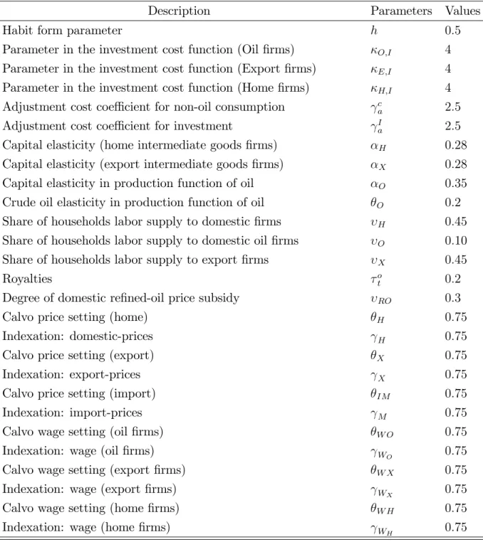
Table 1.2 Calibration of structural parameters (continued)

Description Parameters Values

Habit form parameter h 0:5

Parameter in the investment cost function (Oil …rms) O;I 4

Parameter in the investment cost function (Export …rms) E;I 4

Parameter in the investment cost function (Home …rms) H;I 4

Adjustment cost coe¢ cient for non-oil consumption c

a 2:5

Adjustment cost coe¢ cient for investment Ia 2:5

Capital elasticity (home intermediate goods …rms) H 0:28

Capital elasticity (export intermediate goods …rms) X 0:28

Capital elasticity in production function of oil O 0:35

Crude oil elasticity in production function of oil O 0:2

Share of households labor supply to domestic …rms H 0:45

Share of households labor supply to domestic oil …rms O 0:10

Share of households labor supply to export …rms X 0:45

Royalties o

t 0:2

Degree of domestic re…ned-oil price subsidy RO 0:3

Calvo price setting (home) H 0:75

Indexation: domestic-prices H 0:75

Calvo price setting (export) X 0:75

Indexation: export-prices _X 0:75

Calvo price setting (import) IM 0:75

Indexation: import-prices _M 0:75

Calvo wage setting (oil …rms) W O 0:75

Indexation: wage (oil …rms) WO 0:75

Calvo wage setting (export …rms) W X 0:75

Indexation: wage (export …rms) WX 0:75

Calvo wage setting (home …rms) W H 0:75

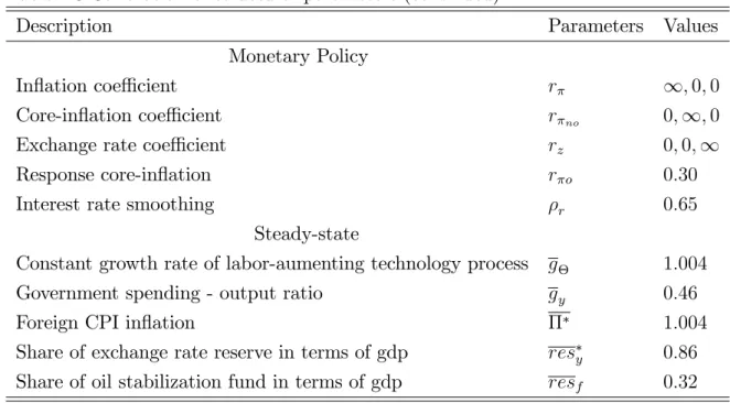
Table 1.3 Calibration of structural parameters (continued)

Description Parameters Values

Monetary Policy

In‡ation coe¢ cient r _{1; 0; 0}

Core-in‡ation coe¢ cient r _no 0;_{1; 0}

Exchange rate coe¢ cient rz 0; 0;1

Response core-in‡ation r o 0:30

Interest rate smoothing r 0:65

Steady-state

Constant growth rate of labor-aumenting technology process g 1:004 Government spending - output ratio g_y 0:46

Foreign CPI in‡ation 1:004

Share of exchange rate reserve in terms of gdp res_y 0:86 Share of oil stabilization fund in terms of gdp resf 0:32

5

Is there a Dutch disease e¤ect?

This section analyzes the impulse responses functions of several keys macroeco-nomic variables in the aftermath of an international oil price shock. Importantly, our impulse responses functions investigate the e¤ectiveness of alternative monetary rules to limit a Dutch disease e¤ect by combining them with …scal policy. In our framework, …scal policy rests on two variables: on the one hand, di¤erent values of the parameter of share of oil stabilization fund (OSF hereafter) dedicated to sup-port trading (exsup-port) sector, and, on the other hand, the inclusion of the enhancing productivity coe¢ cient (EPC) associated to public spending as inBerg et al (2013). Three monetary policy rules are calibrated: an in‡ation targeting rule (hereafter IT rule), a …xed exchange rate rule (hereafter ER rule) and domestic oil price in‡ation rule (Frankel rule).

To interpret our results, it important to note that the impulse responses functions related to the baseline model represent the optimal responses of the economy to the oil shocks. In this perspective, to draw lessons about the e¤ectiveness of …scal and monetary policy to limit the Dutch disease e¤ect, we introduce a set of nominal and real frictions. Such frictions lead the economy to respond in a suboptimal way to

shocks. The …nal step is to compare the baseline model and the responses of the model under di¤erent rules. The response of our selected variables will be relative to that of our baseline model. In these cases, this is the gap between both responses (baseline and sticky price-sticky wage models with monetary rules) that will provide information on the occurrence of the Dutch disease e¤ect.

5.1

Impulse Response Analysis

In this sub-section, we assess the e¤ectiveness of alternative monetary rules by stressing the impact of …scal policy on this e¤ectiveness. Assuming that oil pro-duction is largely exogenous with respect to price changes, due not only to the inertia of supply but also to the constraints of OPEC membership, we focus below on responses in trade and non-tradable sectors.

5.1.1 In‡ation targeting regime

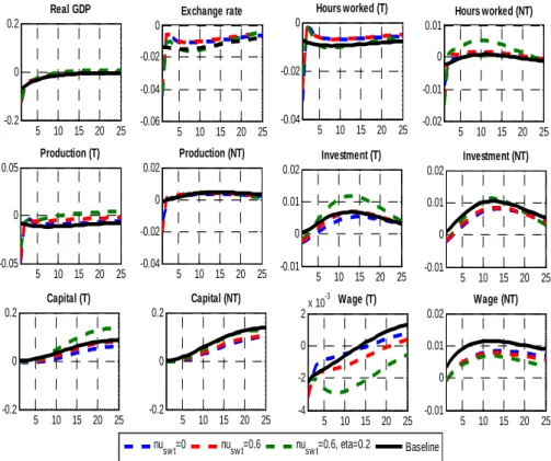
As exhibited in Figure 1, in the aftermath of an international oil price shock, the model gives us an important result. Indeed, the responses of our variables show that the production and investment in the export sector decrease signi…cantly. This suggesting the presence of the deindustrialization phenomenon resulting from oil resource’s abundance. In this case, it seems that the spending e¤ect is active. The spending e¤ect matters to explain the responses of home production and investment in export sector. More speci…cally, the positive oil price shock tends to induce both an increase in capital in‡ows and a rise in the domestic absorption. These two e¤ects lead to a real appreciation of the domestic currency-as capital in‡ows cause a nominal appreciation and non-tradable prices rise with higher domestic absorption-exerting damaging consequences on the competitiveness in the tradable sector.

Importantly, the decline in export sector tends to shrink gradually as the rise in the share of oil stabilization fund dedicated to the support export sector. The decline in export goods production is completely resorbed when we combine the share of OSF with a positive coe¢ cient of enhancing productivity ( ).

Our model shows also that the oil price shock causes a resource movement e¤ect, particularly at short-term. Indeed, hours worked in the export sector and wages in this sector decrease in the aftermath of the shock. Under the in‡ation targeting

framework, while the e¤ectiveness of …scal policy to face the resource movement e¤ect is mixed at short-term, Figures 1 suggests the opposite at a longer horizon. The presence of a OSF in the economy is associated with a rise in hours worked in the export sector.

Overall, targeting in‡ation alone does not spare the economy from the Dutch disease e¤ect. However, combined with …scal policy, we see that the damaging e¤ects of positive oil price shocks are lessened signi…cantly. As expected, the higher the e¢ cacy of public spending-proxied by the value of the productivity enhancing parameter- the higher the e¤ectiveness of the in‡ation targeting.

5 10 15 20 25 -0.2 0 0.2 Real GDP 5 10 15 20 25 -0.06 -0.04 -0.02 0 Exchange rate 5 10 15 20 25 -0.02 -0.01 0 0.01 Hours worked (NT) 5 10 15 20 25 -0.04 -0.02 0 Hours worked (T) nu_{sw t}=0 nu_{sw t}=0.6 nu_{sw t}=0.6, eta=0.2 Baseline 5 10 15 20 25 -0.05 0 0.05 Production (T) 5 10 15 20 25 -0.04 -0.02 0 0.02 Production (NT) 5 10 15 20 25 -0.01 0 0.01 0.02 Investment (T) 5 10 15 20 25 -0.01 0 0.01 0.02 Investment (NT) 5 10 15 20 25 -0.2 0 0.2 Capital (T) 5 10 15 20 25 -0.2 0 0.2 Capital (NT) 5 10 15 20 25 -0.01 0 0.01 0.02 Wage (NT) 5 10 15 20 25 -4 -2 0 2x 10 -3 _{Wage (T)}

Figure 1. Responses to a positive oil price shock (IT rule) 5.1.2 Fixed exchange rate

Figure 2 exhibits a striking result: the …xed exchange rate monetary rule is particularly e¤ective to prevent a Dutch disease e¤ect. Indeed, relative to the base-line model, not only the real GDP and domestic consumption are higher, but we

observe also positive responses of macroeconomic variables related to the export sector. More speci…cally, production and investment in this sector tend to increase over 10 periods relative to the baseline model. As for the in‡ation targeting mon-etary rule, …scal policy heightens the e¤ectiveness of the exchange rate rule. Thus, both production and investment in the export sector improve with the presence of a OSF and a higher productivity enhancing e¤ect associated with public spending. The dynamics of our main macroeconomic variables in the aftermath of a positive oil price shock rests on the two mechanisms of the Dutch disease e¤ect. On the one hand, the exchange rate rule impedes the distortions due to the spending e¤ect. On the other hand, as the real exchange rate does not appreciate after the oil shock, the resource movement e¤ect does not play. For instance, our resultst show that hours worked in the export sector respond positively to the oil shock even if this response is short-lived. However, at short-medium run, the exchange rate rule exhibits better performances than the baseline model. In a similar way, wages and capital increase in the aftermath of the oil shock. These responses are persistent over time.

0 10 20 -0.1 0 0.1 Real GDP 0 10 20 -0.5 0 0.5 Inflation 0 10 20 -0.02 -0.01 0 0.01 Hours worked (T) sw t=0 sw t=0.6 swt=0.6, =0.2 Baseline 0 10 20 -0.02 0 0.02 0.04 Hours worked (NT) 0 10 20 -0.05 0 0.05 Production (T) 0 10 20 -0.04 -0.02 0 0.02 Production (NT) 0 10 20 -0.01 0 0.01 0.02 Investment (T) 0 10 20 -0.01 0 0.01 0.02 Investment (NT) 5 10 15 20 25 0 0.5 1 Capital (T) 5 10 15 20 25 0 0.5 1 Capital (NT) 5 10 15 20 25 0 0.02 0.04 Wage (NT) 5 10 15 20 25 -0.01 0 0.01 0.02 Wage (T)

5.1.3 Real oil price targeting (Frankel rule)

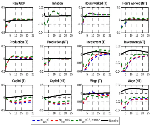
The real oil price shock targeting -the so-called Frankel rule- clearly underper-forms in comparison with the alternative monetary rules. The ine¤ectiveness of the real oil price targeting is especially noticeable at short-medium run as suggested by the dynamics of production and investment in the export e¤ort (Figure 3). We also see that the resource movement e¤ect is e¤ective at short-medium term. Speci…cally, the positive oil shock is associated with a contraction in the export sector through the evolution of capital and wages and hours worked. In addition, our results show that not only the Frankel rule does not prevent the Dutch disease e¤ect but, at the same time, it leads to higher macroeconomic volatility.

Last but not least, unlike other monetary rules, the combination with …scal policy does not improve the e¤ectiveness of monetary policy to cope with the Dutch disease e¤ect. 5 10 15 20 25 -0.5 0 0.5 Real GDP 5 10 15 20 25 -0.04 -0.02 0 0.02 Inflation 5 10 15 20 25 -0.2 -0.1 0 0.1 Hours worked (T) 5 10 15 20 25 -0.1 0 0.1 Hours worked (NT) 5 10 15 20 25 -0.2 0 0.2 Production (T) 5 10 15 20 25 -0.2 0 0.2 Production (NT) 5 10 15 20 25 -0.04 -0.02 0 0.02 Investment (T) nu_{sw t}=0 nu_{sw t}=0.6 nu_{sw t}=0.6, eta=0.2 Baseline 5 10 15 20 25 -0.04 -0.02 0 0.02 Investment (NT) 5 10 15 20 25 -0.5 0 0.5 Capital (T) 5 10 15 20 25 -0.5 0 0.5 Capital (NT) 5 10 15 20 25 -0.04 -0.02 0 0.02 Wage (NT) 5 10 15 20 25 -0.04 -0.02 0 0.02 Wage (T)

5.2

Optimal policy and Welfare analysis

In this sub-section, we evaluate, at the …rst stage, the dynamic of our model under a set of policy rules implemented during a windfall and, at the second stage, the response of welfare to windfall.

5.2.1 Optimal Policy

We compare the reponses of our main variables under alternative monetary and …scal policy rules in the aftermath of an oil price shock. These results are obtained with the standard (or baseline) calibration (see section 2). For this, we use four rules: in‡ation targeting rule (IT rule), …xed exchange rate rule (ER rule), domestic oil price targeting or frankel rule and optimal monetary (OMP) and …scal policies (OFP).

Three lessons are drawn from the analysis of optimal policy. Firstly, in line with …ndings from the impulse responses functions, the real oil price shock targeting exhibits the worst performances. Under this monetary rule, the real GDP is below its stationary level over 7 periods. In a similar way, domestic consumption exhibits a sizable negative dynamics. While the real exchange rate does not appreciate, this movement does not prevent a contraction of export sector as in a typical Dutch disease e¤ect. Thus, investment, capital, wages and hours worked in this sector are consistently below their stationary level. In addition, we see that Frankel rule does not allow macroeconomic stabilization as many of our macroeconomic variables exhibit large ‡uctuations over time.

Secondly, while the …xed exchange rate tends to be associated with ample ‡uc-tuations of macroeconomic variables, the best performances of the export sector is observed in this monetary rule. More speci…cally, all variables related to this sector are persistently above their stationary level. The overall impact of the exchange rate rule is noticeable as both real GDP and domestic consumption stay above their stationary level over the whole period.

Thirdly, other policies, i.e. the in‡ation targeting rule, the optimal monetary policy and the optimal …scal policy, are associated with macroeconomic outcomes located between the two previous policies. On the one hand, these policies are relatively similar in terms of stabilization properties. Thus, real GDP and domestic

consumption as well as export sector variables experience small ‡uctuations around their stationary level. On the other hand, relative to the Frankel rule, these policies perform better in terms of export sector dynamics.

5 10 15 20 25 -0.3 -0.2 -0.1 0 0.1 Real GDP 5 10 15 20 25 -0.15 -0.1 -0.05 0 0.05 Exchange rate 5 10 15 20 25 -0.15 -0.1 -0.05 0 0.05

Hours worked (Export sector)

IT rule ER rule Frankel rule OMP OFP Baseline

5 10 15 20 25 -0.06 -0.04 -0.02 0 0.02 0.04

Hours worked (Home sector)

Figure 4.1 Responses under alternative policy rules

5 10 15 20 25 -0.4 -0.2 0 0.2 0.4 0.6

Capital (Export sector)

5 10 15 20 25 -0.4 -0.2 0 0.2 0.4 0.6

Capital (Home sector)

5 10 15 20 25 -0.03 -0.02 -0.01 0 0.01 0.02

Wage (Export sector)

IT rule ER rule Frankel rule OMP OFP Baseline

5 10 15 20 25 -0.04 -0.02 0 0.02 0.04

Wage (Home sector)

5 10 15 20 25 -0.2 -0.15 -0.1 -0.05 0 0.05

Export goods production

5 10 15 20 25 -0.1 -0.05 0 0.05 0.1 Home production 5 10 15 20 25 -0.04 -0.02 0 0.02 0.04 0.06

Investment (Export sector)

IT rule ER rule Frankel rule OMP OFP Baseline

5 10 15 20 25 -0.04 -0.02 0 0.02 0.04 0.06

Investment (Home sector)

Figure 4.3. (Continued) Responses under alternative policy rules. 5.2.2 Welfare Analysis

To assess the impact of windfall on the welfare, we solve the model using a second order approximation of the utility function for di¤erent policies but also for di¤erent values of two parameters: share of oil stabilization fund dedicated to support trading (export) sector swt;and parameter of productivity enhancing public

capital : Formally, the welfare criterion is derived from the following single utility function: Ut(:) = Bt ln ct hg ;t1ct 1 + M Mt ln (mt) Lt (Lt)1+ 1 + ! (34) As in the impulse response analysis, three monetary policy rules are considered: an in‡ation targeting rule (hereafter IT rule), a …xed exchange rate rule (hereafter ER rule) and domestic oil price in‡ation rule (Frankel rule). In each case, the black, red and blue lines represent the response of the welfare under the baseline model, a positive parameter of share of OSF dedicated to support trading (export) sector, and, the combination of a positive OSF and the enhancing productivity coe¢ cient

0 1 2.5 3 3.5 4 4.5 5x 10

5 _{Welare under ER rule}

Baseline nu_{w st}=0.6 nu_{sw t}=0.6, eta=0.2 0 1 -60 -55 -50 -45 -40 -35

Welfare under Frankel rule

0 1 -20 0 20 40 60 80

Welfare under IT rule

Figure 5. Welfare responses under alternative policy rules

The results are shown in …gure 5. Our main …ndings are in line with the impulse response function’s results. Indeed, under ER rule, the impact of oil price shock generate a welfare gain contrary to IT rule and Frankel rule. The appearance of the Dutch disease in the last two cases seems to have a negative impact on the welfare gain. However, the welfare is negative when monetary authority adopts Frankel rule.

6

Conclusion

In this paper, we studied the role of …scal and monetary policies during a wind-fall episode in an oil exporting economy. Our main purpose was to compare the re-sponses of our model’s variables in the aftermath of a positive oil price shock under three monetary rules (In‡ation targeting rule, Exchange rate peg and Frankel rule) combined with government intervention (a share of oil stabilisation fund dedicated to support trading (export) sector, and the inclusion of the enhancing productivity coe¢ cient (EPC) associated to public spending as in Berg et al (2013). Our main …ndings show that the Dutch disease occurs only under in‡ation targeting and oil price in‡ation rules. The …xed exchange rate monetary rule seems to be e¤ective to prevent a Dutch disease e¤ect. Also, under IT rule, the decline in export sector tends to shrink gradually as the rise in the share of oil stabilisation fund. The decline in export goods production is completely resorbed when we combine the share of OSF with a positive coe¢ cient of enhancing productivity. This is not the case when oil price in‡ation rule is considered. Finally, optimal monetary and …scal policies do not give better results than ER rule which provides also the highest welfare gain.

References

[1] Acosta, P. A., Lartey, E K.K., Mandelman, F. S., 2009. Remittances and the Dutch disease. Journal of International Economics, vol. 79(1), 102-116. [2] Adolfson, M., Laseen, S., Linde, J., Villani, M., 2007. Bayesian estimation of

an open economy DSGE model with incomplete pass-through. Journal of International Economics, vol. 72(2), 481-511.

[3] Alberola, E., Benigno, G., 2017. Revisiting the Commodity Curse: A Financial Perspective. Journal of International Economics, vol 108, Supplement 1, s87-s106.

[4] Alter, A., Ghilardi, M., Hakura, D. S., 2017. Public Investment in Devel-oping Countries Facing Natural Resource Depletion. Journal of African Economies, 26(3): 295–321.

[5] Arezki, R., Ismail, K., 2013. Boom–bust cycle, asymmetrical …scal response and the Dutch disease. Journal of Development Economics, vol. 101(C), 256-267. [6] Baunsgaard, T., Villafuerte, M., Poplawski-Ribeiro, M., Richmond, C., 2012. Fiscal Frameworks for Resource Rich Developing Countries. IMF sta¤ dis-cussion note, 16, 2012 SDN/12/04.

[7] Ben Aïssa, M. S., Rebei, N., 2012. Price subsidies and the conduct of monetary policy. Journal of Macroeconomics, vol. 34(3), 769-787.

[8] Benkhodja, M. T., 2014. Monetary policy and the dutch disease e¤ect in an oil exporting economy. International Economics, 138 , 78-102.

[9] Berg, A., Portillo, R., Yang, S C. S., Zanna, L. F., 2013. Public investment in resource-abundant developing countries. IMF Economic Review, 61(1):92– 129.

[10] Bouakez, H., Rebei, N., Vencatachellum, D., 2008. Optimal Pass-Through of Oil Prices in an Economy with Nominal Rigidities. Cahiers de recherche 0831, CIRPEE.

[11] Calvo, G., 1983. Staggered Prices in a Utility-Maximizing Framework. Journal of Monetary Economics, 12, 383-398.

[12] Cherif, R., 2013. The Dutch disease and the technological gap. Journal of De-velopment Economics 101 (2013) 248-255.

[13] Christiano, L., Eichenbaum, M., Evans, C., 2005. Nominal Rigidities and the Dynamic E¤ects of a Shock to Monetary Policy. Journal of Political Econ-omy, 2005, vol. 113 (1), 1-45.

[14] Christo¤el, K., Coenen, G., Warne, A., 2008. The new Area-Wide model of the euro area: a micro-fouded open-economy model for forcasting and policy analysis. Working paper, vol 0944, ECB.

[15] Dagher, J., Gottschalk, J., Portillo, R., 2012. The Short-run Impact of Oil Windfalls in Low-income Countries: A DSGE Approach, Journal of African Economies (2012) 21 (3): 343-372.

[16] Devereux, M., Lane, P. R., Xu, J., 2006. Exchange Rate and Monetary Policy in Emerging Market Economies. The Economic Journal, 116: 478-506. [17] El Anshasy, AA., Bradley, MD., 2012. Oil prices and the …scal policy response

in oil-exporting countries. Journal of Policy Modeling 34 (5), 605-620. [18] Erceg, C., Henderson, D., Levin, A., 2000. Optimal monetary policy with

stag-gered wage and price contracts. Journal of Monetary Economics 46, 281-313. [19] Erceg, V. J., Guerrieri, L., Gust, C., 2006. SIGMA: A New Open Economy Model for Policy Analysis. International Journal of Central Banking, Inter-national Journal of Central Banking, vol. 2(1).

[20] Frankel, J.A., 2011. A Comparison of Product Price Targeting and Other Mone-tary Anchor Options for Commodity Exporters in Latin America, Economia, 12(1): 1-57.

[21] Frankel, J.A., 2017. The Currency-Plus-Commodity Basket: A Proposal for Exchange Rates in Oil-Exporting Countries to Accommodate Trade Shocks Automatically, HKS Working Paper No. RWP17-034.

[22] IMF., 2012. Macroeconomic Policy Frameworks of Resource-Rich Developing Countries, Sta¤ team report led by D. Ghura and C. Pattillo, August 24th, Washington D.C.

[23] Jacquinot, Pascal and Mestre, Ricardo and Spitzer, Martin, An Open-Economy DSGE Model of the Euro Area (July 2006). Available at SSRN: https://ssrn.com/abstract=951504 or http://dx.doi.org/10.2139/ssrn.951504

[24] Lama, R., Medina, J. P., 2012. Is Exchange Rate Stabilization an Appropriate Cure for the Dutch Disease? International Journal of Central Banking, International Journal of Central Banking, vol. 8(1), 5-46.

[25] Monacelli, T., 2005. Monetary Policy in a Low Pass-Through Environment. Journal of Money, Credit and Banking, vol 37, (6), 1047-1066.

[26] Pieschacón, A., 2012. The value of …scal discipline for oil-exporting countries. Journal of Monetary Economics, vol. 59(3), 250-268.

[27] Schmitt-Grohé, S., Uribe, M., 2003. Closing Small Open Economy Models. Journal of International Economics, 61: 163-185.

[28] Smets, F., Wouters, R., 2003. An Estimated Dynamic Stochastic General Equi-librium Model of the Euro Area. Journal of the European Economic Asso-ciation, vol. 1(5), 1123-1175, 09.

[29] Stahler, N., and Thomas, C., 2012. FiMod-a DSGE model for …scal policy simulations. Economic modelling, vol 29(2), 239-261.

A

Appendix

Table 2. Oil export in total export

Upper-Middle-Income High-Income Lower-Middle-Income Algeria Venezuela Russia Ecuador Norway Canada Angola Congo

1990 96,5 80,1 51,9 47,8 10,0 93,5 89,1 1995 94,6 76,7 43,11* 35,9 47,3 9,2 94,8 87,6 2000 97,2 86,1 50,6 49,4 63,9 14,2 94,8 87,6 2005 98,0 88,0 61,8 58,4 67,7 21,6 96,5 67,7 2010 97,3 93,4 65,6 55,3 63,8 26,3 96,6 77,7 2013 96,7 97,7 71,2 57,0 67,7 27,3 97,2 78,9 Average 96,8 88,4 62,3 51,2 62,1 19,7 96,0 79,9 Table 3. Oil export in term of GDP

Upper-Middle-Income High-Income Lower-Middle-Income Algeria Venezuela Russia Ecuador Norway Canada Angola Congo 1990 20,0 29,1 16,0* 11,6 9,9 2,0 32,5 39,7 1995 23,1 17,9 5,4 6,7 10,2 2,4 64,5 45,6 2000 38,5 23,7 13,0 13,3 17,2 4,7 77,0 74,9 2005 44,1 33,6 14,3 14,1 14,6 6,0 80,9 72,5 2010 34,8 21,2 12,6 13,9 10,9 5,0 58,8 70,4 2014 30,6 39,4 12,9 14,1 9,9 6,2 53,6 61,2 Table 4. Government e¤ectiveness

Upper-Middle-Income High-Income Lower-Middle-Income Algeria Venezuela Russia Ecuador Norway Canada Angola Congo 1996 -1,089 -0,541 -0,452 -0,475 1,951 1,742 -0,860 -1,169 2000 -0,964 -0,737 -0,720 -0,766 1,897 1,931 -1,462 -1,265 2005 -0,468 -0,931 -0,500 -0,947 1,864 1,887 -1,137 -1,271 2010 -0,480 -1,112 -0,469 -0,717 1,879 1,783 -1,118 -1,228 2016 -0,545 -1,293 -0,216 -0,432 1,883 1,798 -1,039 -1,096 Average -0,662 -0,988 -0,443 -0,678 1,905 1,838 -1,163 -1,189

Documents De travail GreDeG parus en 2018

GREDEG Working Papers Released in 2018

2018-01 Lionel Nesta, Elena Verdolini & Francesco Vona

Threshold Policy Effects and Directed Technical Change in Energy Innovation

2018-02 Michela Chessa & Patrick Loiseau

Incentivizing Efficiency in Local Public Good Games and Applications to the Quantification of

Personal Data in Networks

2018-03 Jean-Luc Gaffard

Monnaie, crédit et inflation : l’analyse de Le Bourva revisitée

2018-04 Nicolas Brisset & Raphaël Fèvre

François Perroux, entre mystique et politique

2018-05 Duc Thi Luu, Mauro Napoletano, Paolo Barucca & Stefano Battiston

Collateral Unchained: Rehypothecation Networks, Concentration and Systemic Effects

2018-06 Jean-Pierre Allégret, Mohamed Tahar Benkhodja & Tovonony Razafindrabe