HAL Id: halshs-00983063
https://halshs.archives-ouvertes.fr/halshs-00983063
Submitted on 24 Apr 2014HAL is a multi-disciplinary open access
archive for the deposit and dissemination of sci-entific research documents, whether they are pub-lished or not. The documents may come from
L’archive ouverte pluridisciplinaire HAL, est destinée au dépôt et à la diffusion de documents scientifiques de niveau recherche, publiés ou non, émanant des établissements d’enseignement et de
Optimal Rationing within a Heterogeneous Population
Philippe Choné, Stéphane Gauthier
To cite this version:
Philippe Choné, Stéphane Gauthier. Optimal Rationing within a Heterogeneous Population. 2014. �halshs-00983063�
Documents de Travail du
Centre d’Economie de la Sorbonne
Optimal Rationing within a Heterogeneous Population
Philippe CHONÉ, Stéphane GAUTHIER
Optimal Rationing
within a Heterogeneous Population
Philippe Chon´e
∗CREST-ENSAE
St´ephane Gauthier
†PSE and University of Paris 1
January 1, 2014
Abstract
A government agency delegates to a provider (hospital, medical gatekeeper, school, social worker) the decision to supply a service or treatment to individual recipients. The agency does not perfectly know the distribution of individual treatment costs in the population. The single-crossing property is not satisfied when the uncertainty per-tains to the dispersion of the distribution. We find that the provision of service should then be distorted upwards relative to efficiency when the (first-best) efficient number of recipients is sufficiently high. JEL classification numbers: I18, D82, D61
Keywords: Rationing, screening, universal coverage, upward distor-tion, Spence-Mirrlees condition
∗ENSAE, 3 avenue Pierre Larousse, 92245 Malakoff; Phone: +33(0)141175390; E-mail
address: [email protected].
†MSE, 106-112 bd de l’Hˆopital, 75013 Paris, France; Phone: +33(0)144078289; E-mail
1
Introduction
We consider a government agency in charge of supplying a service or treat-ment to a population of potential recipients. We assume that the cost and the benefit of the treatment vary across individuals. Efficiency requires that the treatment is provided to an individual if and only if social benefit exceeds social cost for that individual.
The individual heterogeneity in cost and benefit may in part be explained by recipients’ characteristics that are observed by the agency. To some extent, the agency can thus use “rationing by denial”, whereby the treatment is denied to individuals with unfavorable cost-benefit ratio. In many instances, however, there remains substantial unobserved heterogeneity conditional on observable variables. The agency has then to leave the selection of recipients to the discretion of the service provider, i.e. rely on “rationing by selection”, see [3]. In practice, the supply decision is indeed delegated to the provider for various services, e.g. medical or social care, after-school or training programs. Under rationing by selection, the agency first determines the total num-ber of recipients. This step requires knowing the distribution of unobserved heterogeneity among potential recipients. Perfect knowledge of the distribu-tion is commonly assumed in the literature. For instance, the assumpdistribu-tion is made in [5] and [4], with the former article considering many treatment vari-eties and the latter investigating provider altruism –two issues not addressed here.
The present note places the emphasis on the uncertainty about the dis-tribution of unobserved heterogeneity. The composition of the population of recipients addressed by a given provider depends on local conditions, creat-ing significant variation in the underlycreat-ing distributions across providers. The effect of differences in composition on the cost and benefit distributions is difficult to estimate empirically (see [6] for a recent survey).
Accordingly, we relax the assumption that the agency perfectly knows the cost and benefit distribution in the population of potential recipients. We find that the uncertainty about the distribution of heterogeneity causes the number of recipients to be distorted relative to efficiency. The direction of the distortion depends on whether the uncertainty pertains to the mean or to the dispersion of individual treatment costs. In the former case, the usual Spence-Mirrlees condition is satisfied and the distortion is necessarily downwards: The number of treated recipients is lower than recommended
by first-best efficiency. In the latter case, the Spence-Mirrlees condition no longer holds. We find that the first-best optimum governs the the sign of distortion in the second-best program: The distorsion is upwards when the first-best number of treated recipients is sufficiently high. Uncertainty about the cost dispersion then pushes towards universal coverage policies.
2
Model
A population of recipients, whose size is normalized to one, is eligible for a treatment supplied by a single provider. Recipients are indexed by two nonnegative real numbers b and c, with distribution function Φ(b, c). The treatment of a type (b, c) recipient yields benefit b to the recipient and costs c to the provider. The corresponding net social benefit is b − (1 + λ)c, where λ is the (exogenously given) marginal cost of public funds.
Assumption 1. The (expected) net social benefit of treatment for a given cost level c, E(b | c) − (1 + λ)c, is a non-increasing function of cost c with a unique zero, denoted by c∗∗
.
Assumption1holds true in particular when the expected benefit decreases with cost, a case often considered in the literature, e.g., in [2] and [4]. [5] provides health related examples where this assumption is relevant. Under this assumption, the first-best requires to treat recipients with cost c ≤ c∗∗
. Denoting by F the marginal distribution of individual treatment costs in the population of recipients, the first-best optimal number of treated recipients is n∗∗
= F (c∗∗
).
In this paper, we assume that the agency relies on rationing by selec-tion: the agency observes the number n of recipients but not their individual characteristics. The treatment decision is delegated to a single provider who observes the individual characteristics of recipients. The agency offers a take or leave contract specifying the number of recipients that must be treated by the provider and a compensating transfer T . The utility of the provider when she accepts the contract is U (n, T ) = T − C(n), where C(n) represents the aggregate cost of treating n recipients.
Given (n, T ), utility maximization requires that the least costly recipients be treated in priority. The provider’s cost of treating n recipients, 0 ≤ n ≤ 1,
is therefore given by
C(n) =
Z F−1(n)
0
c dF (c). The marginal cost is C′
(n) = F−1
(n), i.e., the cost of the marginal treated recipient is F−1
(n), the nth-percentile of the distribution F . It follows that the cost function C(n) is convex in n.
The net social benefit of treating n recipients is given by S(n) = B(n) − (1 + λ)C(n), where
B(n) =
Z F−1(n)
0 E(b | c) dF (c).
represents the (expected) the gross social benefit. Under Assumption 1, the net social benefit function S(n) is concave in n, reaching its maximum at n∗∗
= F (c∗∗
). When the agency knows the distribution of individual recipients characteristics Φ, it can choose the number of recipients n and the transfer T that maximize
B(n) + U (n, T ) − (1 + λ)T = S(n) − λU (n, T )
subject to the provider’s participation constraint U (n, T ) ≥ 0. The solution to this maximization problem is the first-best optimum, n = n∗∗
and U = U∗∗
= 0.
Under Assumption 1, the provider treats in priority the recipients with highest expected social values: The social net benefit and the provider’s private objective are ‘aligned.’ Hence, the agency can achieve the first-best optimum if it knows the distribution of individual recipients characteristics: From the distribution function Φ, the agency infers the optimal number n∗∗
and the corresponding cost, C(n∗∗
). It is then sufficient to ask the provider to treat n∗∗
recipients and reimburse C(n∗∗
).
3
Unknown cost distribution
We now relax the assumption that the agency knows the distribution of indi-vidual characteristics of recipients. We suppose that the agency only knows that the distribution function is Φi (i = H, L), associated with marginal cost
distribution Fi, with probability πi (πL + πH = 1). The true distribution
type. Hence, the agency is faced with two types of provider, themselves con-fronted with different populations of recipients and marginal distributions of individual costs. Provider i has cost function Ci(n) with Ci′(n) = F
−1 i (n),
and the net social benefit of having n recipients treated by provider i is Si(n) =
Z Fi−1(n)
0
[ Ei(b | c) − (1 + λ)c ] dFi(c),
where the conditional expectation Ei is taken under provider i’s
distribu-tion Φi. Assumption 1 is supposed to hold for the two provider types: The
first-best cost threshold for provider i is c∗∗
i such that Ei(b | c∗∗i ) = (1 + λ)c ∗∗ i ,
where Ei(b | c ∗∗
i ) represents the mean treatment benefit for provider i in
the population of recipients whose treatment cost is c∗∗
i . The corresponding
first-best number of recipients is n∗∗
i = Fi(c∗∗i ).
Appealing to the revelation principle, the agency offers a menu (ni, Ti),
i = H, L, maximizing
X
i
πi[Si(ni) − λUi(ni, Ti)]
subject to the provider’s participation constraints Ui(ni, Ti) = Ti−Ci(ni) ≥ 0
and the incentive constraints Ui(ni, Ti) ≥ Ui(nj, Tj) for all i, j = H, L.
We examine how the solution to this problem departs from the first-best optimum when the marginal distribution FL stochastically dominates the
distribution FH.
3.1
Local distortions
Suppose first that FLfirst-order stochastically dominates FH: FL(c) ≤ FH(c)
for all c, with strict inequality on a non-degenerated interval. In this case, for all n > 0, provider H’s marginal cost stands below provider L’s:
C′ H(n) = F −1 H (n) < C ′ L(n) = F −1 L (n),
and hence CH(n) < CL(n), since CH(0) = CL(0). The first-best menu
(n∗∗ i , Ci(n
∗∗
i )) is not incentive compatible: Provider H chooses (n ∗∗ L, CL(n ∗∗ L)) and earns CL(n ∗∗ L) − CH(n ∗∗
L) > 0. In order to reduce the informational rent
of recipients treated by type L with respect to the first-best n∗∗
L. The usual
single-crossing condition is satisfied: ∂T ∂n UH = C′ H(n) < C ′ L(n) = ∂T ∂n UL for all n.
Therefore a lower rent requires a lower number of recipients treated by provider L. This is the standard pattern in adverse selection problems. Proposition 1. Suppose that FL first-order stochastically dominates FH. At
the second-best optimum, provider H (provider L) treats the optimal number of (too few) recipients and earns a positive (zero) profit.
Proof. Since CL(n) > CH(n), the type H incentive constraint is binding,
U∗ H = CL(n ∗ L) − CH(n ∗ L), and U ∗
L = 0. The optimal number n ∗ L satisfies the first-order condition πLS ′ L(n ∗ L) − λπH[C ′ L(n ∗ L) − C ′ H(n ∗ L)] = 0. (1) Thus S′ L(n ∗ L) > 0 = S ′ (n∗∗
L), and S(n) being single-peaked, n ∗ L < n ∗∗ L. Type H treats n∗ H = n ∗∗
H recipients and earns U ∗ H = CL(n ∗ L) − CH(n ∗ L) > 0.
The main result of the paper concerns the case where FH is a
mean-preserving spread of FL: Both distributions FH and FL have the same mean,
CL(1) = Z ∞ 0 c dFH(c) = Z ∞ 0 c dFL(c) = CH(1),
and FL second-order stochastically dominates FH,
Z c 0 FL(c) dc ≤ Z c 0 FH(c) dc for all c.
Assumption 2. The two distribution functions cross only once, at some individual treatment cost denoted ˆc.
The single-crossing property does not hold, but Assumption 2 restricts the pattern of violation of this assumption, delimitating two different regions:
∂T ∂n UH = C′ H(n) < C ′ L(n) = ∂T ∂n UL ⇐⇒ n < ˆn, (2)
with ˆn = FL(ˆc) = FH(ˆc). In the spirit of [1], we use this partition to handle
the adverse selection problem.1
Proposition 2. Suppose that FH is a mean-preserving spread of FLand that
Assumption 2 holds. Then, provider’s H incentive constraint is the only one to be binding at the optimum. This provider treats n∗∗
H recipients.
The agency has a local incentive to distort the number of recipients treated by provider L upwards from n∗∗
L if and only if n ∗∗ L > ˆn.
Proof. By Assumption 2, FH(c) > FL(c) for c < ˆc and FH(c) < FL(c) for
c > ˆc. Using the expression of the marginal costs, we find that C′
H(n) < C′ L(n) for n < ˆn and C ′ H(n) > C ′
L(n) for n > ˆn. Since CH(0) = CL(0) and
CH(1) = CL(1), we have
CH(n) ≤ CL(n)
for all n, with equality for n = 0 and n = 1. The cost difference CL(n)−CH(n)
first increases, then decreases as n rises, achieving its maximum at ˆn = FH(ˆc) = FL(ˆc). The efficient provider, provider H, is the one faced with
more dispersed individual treatment costs.
It follows that at the second-best optimum, H’s incentive constraint must be binding, U∗ H = CL(n ∗ L) − CH(n ∗ L), and U ∗
L = 0. The number of recipients
treated by provider H is undistorted. The optimal number n∗
L of treated by
the L type maximizes
K(n) ≡ πLSL(n) + λπH[CH(n) − CL(n)]. (3)
The first derivative of this function at n∗∗
L is λπH[C ′ H(n ∗∗ L) − C ′ L(n ∗∗ L)], since
SL(n∗∗L) = 0. By (2), it is positive if and only if n ∗∗ L > ˆn.
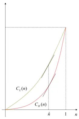
Figures 1 and 2describe how to derive the aggregate cost function from the marginal distribution of individual cost. By Assumption 2the marginal distributions intersect at ˆc. From the second order stochastic dominance property we also know that FH(c) is above (below) FL(c) for c less (greater)
than ˆc. Therefore, the slope of the cost function for provider H is less (greater) than the slope of the cost function for provider L when n is less (greater) than ˆn. This change in the way the slopes are ordered implies a fail-ure of the usual single-crossing condition. However, given that both providers
1In our setup, however, C′
H(n) − CL′(n) is non-monotonic in n, hence [1]’s Assumption
1 ) (c FL ) (c FH(c) FH nˆ c ) ˆ ( ) ˆ ( 1 1 n F n FH L
Figure 1: Individual cost cdf
) (n CL ) (n CH ˆ n nˆ 1
0 ) , (T n U L(T,n) 0 U L 0 ) , (T n U H ˆ * * * n nˆ 1 L n L n
Figure 3: Downward distortion
0 ) , (T n UH 0 ) , (T n UL ˆ ** * n nˆ nL nL1
Figure 4: Upward distortion
have the same aggregate costs at n ∈ {0, 1}, provider’s H aggregate cost must be lower for all n ∈ (0, 1).
The intuition is simple: When n recipients are treated, the individual treatment costs are concentrated around the mean CL(1) for provider L
and are more dispersed for provider H. The latter provider treats in pri-ority the least costly recipients, which gives him a cost advantage relative to provider L, that advantage being maximal for n = ˆn. Though the single-crossing condition is not met, type L (H) is unambigously the ‘inefficient’ (‘efficient’) type, i.e., CL(n) ≥ CH(n) for all n, thus allowing us to handle
with incentive constraints.
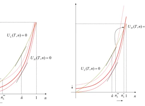
Figures3and4illustrate how the failure of the Spence-Mirrlees condition can be exploited by the agency to reduce the type H informational rent CL(nL) − CH(nL). The iso-utility curves are increasing and convex in n. In
the first-best, both types would earn zero utility: The corresponding iso-utility curves pass through the origin n = T = 0. If the first-best contracts were offered, type H would imitate type L by choosing to treat n∗∗
L recipients.
Provider H would then earn a positive profit T∗∗
L − CH(n ∗∗
L) = CL(n ∗∗ L) −
has a local incentive to reduce the number of treated by the L type when n∗∗
L < ˆn, as is the case in Figure 3. On the contrary, n ∗∗
L > ˆn in Figure 4,
and the agency then has a local incentive to increase the number of treated above n∗∗
L.
Thus, unlike the main strand of the literature, the sign of the local dis-torsion from the first-best optimum in the second-best setup are driven by the number of treated in the first-best problem: A high number of treated in the first-best yields an upward distorsion.
3.2
A global result
Previous results describe the pattern of local incentives to distort the number of treated recipients from the first-best. However it could be that the global optimum involves to treat n∗
L < n ∗∗
L recipients in the case where n ∗∗
L is above
ˆ
n. To go beyond the local result of Proposition 2, we introduce
Assumption 3. The distributions FL and FH are symmetric around ˆc, i.e.
Fi(c) + Fi(2ˆc − c) = 1 for all c and i = H, L.
Under Assumptions2and 3, the distributions are equal to one half when they cross: ˆn = FH(ˆc) = FL(ˆc) = 1/2.
Proposition 3. Suppose that Assumptions 2 and 3 hold, FH is a
mean-preserving spread of FL, and n ∗∗
L is larger than 1/2. Then the number of
recipients treated by provider L is distorted upwards if SL(1) > SL(1 − n ∗∗ L).
Proof. By Assumption3, the rent UH(nL) = CL(nL) − CH(nL) is symmetric
around its global maximum ˆn = 1/2, i.e. UH(n) = UH(1 − n) for all n.
Recall that the second-best number n∗
L of recipients treated by provider L
maximizes the function K(n) given by (3). We want to show that n∗ L> n
∗∗ L
when n∗∗
L > 1/2. The proof proceeds in three steps:
1. Let ˜nL = 1 − n∗∗L < 1/2. Since UH(n) = UH(1 − n) and SL increases
below n∗∗
L, the maximum of K on [˜nL, n ∗∗
L] is achieved above 1/2.
2. Since SL is increasing and UH is decreasing on the interval [1/2, n ∗∗ L],
K is increasing on this interval, implying that the maximum of K on [˜nL, n
∗∗
L] is achieved at n ∗∗ L.
3. By symmetry of UH and monotonicity of SL on the intervals [0, n ∗∗ L] and [n∗∗ L, 1], we have K(n) − K(1 − n) = SL(n) − SL(1 − n) ≥ SL(1) − SL(1 − n ∗∗ L) > 0 for all n ≥ n∗∗
L. It follows that the maximum of K(n) on [0, 1] is
achieved at the right of n∗∗ L.
By Proposition 2, the maximum is achieved strictly above n∗∗ L.
This global result is closely reminiscent of Proposition 2: The number of recipients is distorted upwards from the first-best optimum if the agency prefers the inefficient provider (the one faced with less dispersed individual treatment costs) to treat a sufficiently high number of recipients.
The new global condition in Proposition 3 depends on whether treating all the population is socially preferred to treating only a fraction 1 − n∗∗
L. It
should be satisfied in practice: if the first-best optimum recommends to treat n∗∗
L = 80% of the population, the agency should prefer providing universal
coverage to treating only 1 − n∗∗
L = 20% of the population.2
References
[1] Araujo, A., and H. Moreira (2010): “Adverse selection problems without the Spence-Mirrlees condition,” Journal of Economic Theory, 145(3).
[2] De Fraja, G. (2000): “Contracts for health care and asymmetric infor-mation,” Journal of Health Economics, 19, 663–677.
[3] Klein, R., and J. Mayblin(2012): “Thinking about rationing,” Dis-cussion paper, The King’s Fund.
[4] Makris, M., and L. Siciliani (2013): “Optimal incentive schemes for altruistic providers,” Journal of Public Economic Theory, 15(5), 675–699.
2This condition follows from Assumption3. Global results involving an upwards
distor-tion obtain for asymmetric distribudistor-tions when, for high values of n (n > ˆn), the first-best surplus for the inefficient provider is sufficiently high, and the difference between the ag-gregate cost functions of both providers decreases sufficiently with n.
[5] Malcomson, J. (2005): “Supplier Discretion over Provision:Theory and an Application to Medical Care,” RAND Journal of Economics, 36(2). [6] Street, A., D. Scheller-Kreinsen, A. Geissler, and R. Busse
(2010): “Determinants of hospital costs and performance variation: Meth-ods, models and variables for the EuroDRG project,” Working Papers in Health Policy and Management 3.