Non-anonymous Growth Incidence Curves, Income Mobility and Social Welfare Dominance : a theoretical framework with an application to the Global Economy

HAL Id: halshs-00966324

https://halshs.archives-ouvertes.fr/halshs-00966324

Preprint submitted on 26 Mar 2014

HAL is a multi-disciplinary open access

archive for the deposit and dissemination of sci-entific research documents, whether they are pub-lished or not. The documents may come from teaching and research institutions in France or

L’archive ouverte pluridisciplinaire HAL, est destinée au dépôt et à la diffusion de documents scientifiques de niveau recherche, publiés ou non, émanant des établissements d’enseignement et de recherche français ou étrangers, des laboratoires

Non-anonymous Growth Incidence Curves, Income

Mobility and Social Welfare Dominance : a theoretical

framework with an application to the Global Economy

François Bourguignon

To cite this version:

François Bourguignon. Non-anonymous Growth Incidence Curves, Income Mobility and Social Welfare Dominance : a theoretical framework with an application to the Global Economy. 2010. �halshs-00966324�

Non-anonymous Growth Incidence Curves,

Income Mobility and Social Welfare Dominance:

a theoretical framework with an application

to the Global Economy

François BOURGUIGNON

Paris School of Economics

March 2010

G-MonD

Working Paper n°14

Non-anonymous Growth Incidence Curves,

Income Mobility and Social Welfare Dominance:

a theoretical framework with an application to

the Global Economy

François Bourguignon

Paris School of Economics

March 2010

Abstract

The distributional incidence of growth is generally analyzed by com-paring the quantiles of the pre- and post-growth income distribution -e.g. the so-called Growth Incidence Curves. Such an approach based on an implicit re-ranking of individual incomes ignores income mobility by as-suming that only post-growth income matters in social welfare. By con-trast, this paper takes the view that "status quo matters" and that social welfare should logically be defined on both inital and terminal income. This leads to consider ’non-anonymous’ Growth Incidence Curves that plot income growth rates against the various quantiles of the initial dis-tribution. Dominance criteria that generalize those available for standard growth incidence curves are derived, which account for the inequality of individual income growth rates, conditional on initial income. An applica-tion to the cross-country distribuapplica-tional feature of global growth illustrates the analysis.

1

Introduction

Growth incidence curves (GIC) are increasingly used to describe the distribu-tional effects of growth. They simply plot the mean growth rate of real income in a population against income quantiles - see figure 1. A downard sloping GIC. thus indicates that growth contributes to equalizing the distribution of income and vice-versa for an upward sloping curve. Of course, the shape of GICs may be very diverse. An important issue, therefore, is that of comparing different

∗_{Paper prepared for the Conference "Inequality: new directions", Cornell University and}

London School of Economics, Ithaca 11-13 September 2009. I thank the participants to the conference for very helpful comments.

GIC. Under which circumstances, is it possible to say that a growth episode or its GIC is "better" than another, and what is the meaning of such a statement? Answers to that question have been provided by Ravallion and Chen (2003) and Son (2004). They essentially rely on applying first-order and second-order dominance criteria - Atkinson (1970) - to the terminal distribution of income. For instance, first order dominance implies that the GIC of a growth spell is everywhere above that of another. Second order dominance requires the mean growth rate of the p poorest in a growth episode or the ’pcumulative GIC’ -be everywhere larger than in another.

These results are quite intutitive. Growth may be thought as a specific re-distribution process, which can be analyzed with the standard tools of income redistribution analysis - i.e. tax-benefit incidence. In particular, GICs are very similar to tax progressivity charts whereas cumulative GIC bears some resem-blance with "concentration curves".1

On second thought, there is a difference, though. It lies in the horizontal axis of GICs. In standard redistribution analysis, individuals are ranked according to their position in the initial distribution of income.and the incidence curve shows how much their income is modified by redistribution. An important issue that arises in this context is that of the ’re-ranking’ of individuals by the redistrib-ution system. Many results on the relativive "progressivity’ of a redistribredistrib-ution system visavis another are valid only if there is no reranking of individuals -see Lambert (1993) for instance.

GICs compares the income of individuals which were not necessarily in the same initial position. The cumulative GIC shows the difference between the initial income of those individuals who are initially among the p poorest and the income of the p poorest individuals in the terminal distribution. They are not necessarily the same individuals. As redistribution analysis when it excludes re-ranking, GICs somehow ignore the issue of income mobility. Yet, GICs may have different shapes depending on whether mean growth rates are measured before or after the re-ranking of the population - see figure 3 below.

The present paper analyzes the distributional incidence of growth using the initial distribution as a reference, which leads to define ’non-anonymous’ Growth Incidence Curves (na-GIC). This extension of the original analysis of the distri-butional features of growth logically leads to taking into account the full joint distribution of individual initial incomes and terminal incomes, or equivalently, initial income and income growth, or income change As with GICs, the goal is to define dominance criteria of a growth path over another. Reasonably enough, the comparison is restricted to growth paths with the same initial distribu-tion, which we shall then call ’growth processes’ by analogy with the ’income processes’ defined by Benabou and Ok ( 2001).

Results similar to dominance criteria with GICs are obtained when social welfare functions are defined exclusively on final income. But things are different when it is recognized that "status quo matters", or, in other words, social welfare is defined on the bi-dimensional distribution of both initial and terminal incomes

as assumed in part of the literature on income mobility - e.g. Atkinson (1983), Chakravrty et al. (1985), Dardanoni (1993) or Gottschalk and Spolaore (2003) among others. In that case, it is shown that the GIC dominance criteria has to be complemented by more restrictive criteria. In particular, social welfare dominance requires not only dominance of the cumulative na-GICs but also that of "inequality corrected cumulative na-GICs". Although a direct application of the sequential dominance criterion obtained by Atkinson and Bourguignon (1986), these criteria do not seem to ever have been made explicit.2

Several authors already pointed to the difference that it makes to re-rank income earners or not to re-rank them in drawing growth incidence curves and in comparing growth spells. In analyzing the pro-poorness of growth in differ-ent countries based on panel data on individual incomes Jenkins and van Kern (2006, 2008) or Grimm (2007) have shown how different conclusions were ob-tained when using standard GICs and what we call in this paper non-anonymous GICs. If they discussed the issue of dominance of one growth episode over an-other based on non-anonymous GIC, however, they do not deal with the full implications of taking simultaneously into account both initial and terminal incomes in the evaluation of social welfare.

The paper is organized as follows. The next section recalls the basic results about GIC dominance relying on simple empirical examples based on the cross-country distribution of global growth in different periods. Section 3 presents sufficient and necessary conditions for the dominance of one growth process over another for general classes of social welfare functions defined on initial in-come and inin-come change and for a given initial ditribution of inin-come. These conditions imply in turn dominance criteria for na-GICs and for an extension of na-GIC that takes into accoun the inequality of income changes conditionally on initial income. Links with GIC dominance are also discussed. The analysis is conducted with continuous distributions and is shown to combine standard one-dimensional dominance results in the terminal income space and income-mobility specific criteria. Section 4 illustrates those various dominance condi-tions with a comparison of the cross-country structure of global economic growth in two recent periods using the 1995 distribution of world income as common initial reference. The concluding section summarizes the various results in the paper.

2

Alternative representations of the distributional

incidence of growth

Let the initial distribution of income in the economy being studied be described by its density, f (y), and cumulative distribution function F (y), with support (0, a). Growth takes place over some time period. Its distributional impact may

2_{Fields et al. (2002) refer explicitly to stochastic dominance of a distribution of income}

be described by the conditional distribution function, e_{Φ(z | y) of terminal} in-comes, z, conditionally on initial incomes y. Finally, let Φ(z) be the marginal distribution of income at terminal time implied by eΦ( ). We are interested in comparing two growth paths described by the transition functions eΦ( ) and e

Φ∗_{( ) and their corresponding terminal distributions Φ(z) and Φ}∗_{(z). Unless}

specified otherwise, we shall assume that the two growth paths have the same initial distribution, F (y).

Growth incidence curves are defined on the initial and terminal distributions of income. Define the ’quantile function’, yF(p) as the inverse of the cumulative

density F ():

yF(p) ⇐⇒ p = F (y)

and similarly for the terminal distribution Φ() or Φ∗_{(). The Growth Incidence}

Curve corresponding to the growth path Φ may then be defined (Ravallion and Chen, 2003) as:

gΦF(p) =

yΦ(p)

yF(p)− 1

It simply shows the rate of growth of the pth _{quantile of the distribution. The}

distributional impact of growth is thus represented through the inverse of the cumulative distribution functions rather than those functions themselves.

An obvious property of the GIC is First Order Dominance. Assume that the terminal distribution Φ() first order dominates (F OD) that of the alternative growth path Φ∗_{( ). In other words, the (additive) social welfare associated with}

Φ() is larger or equal to that associated with Φ∗_{( ) for all individual income}

utility functions that are increasing. It is well known that this is equivalent to Φ(z) ≤ Φ∗_{(z) for all z. This in turn implies that the GIC associated with}

growth path eΦ must be everywhere above that corresponding to growth path e

Φ∗_{, as long, of course, as initial distributions are the same on the two growth}

paths. Formally:

Φ() F OD Φ∗_{() ⇐⇒ Φ(z) ≤ Φ}∗_{(z) ∀z ⇐⇒ g}ΦF(p) ≥ gΦ∗_F(p) ∀p

Second order social welfare dominance (SOD) refers to individual utility functions that are increasing and concave in income. It is equivalent to the integral of the cumulative density function Φ() being no larger than the integral of Φ∗( ). In turn, we know this is equivalent to the mean income of the p poorest, or the ’generalized Lorenz curve’, being no smaller with Φ() than with Φ∗_{() for}

all p. Using quantile functions, the Generalized Lorenz curve can be expressed as : e LΦ(p) = Z p 0 yΦ(q)dq

Using the GIC, this can be rewritten as: e LΦ(p) = Z p 0 [gΦF(q) + 1] yF(q)dq = Z p 0 gΦF(q)yF(q)dq + eLF(p)

Comparing social welfare associated with two growth paths Φ and Φ∗, we thus have: Φ() SOD Φ∗_{() ⇐⇒} Z p 0 xΦ(q)dq ≥ Z p 0 xΦ∗(q)dq f or all p

where xΦ(q) is the absolute - rather than relative - change in quantile income

q over the growth path Φ, and similarly for Φ∗_{. Equivalently, this relationship}

may also be expressed in terms of the ’p-cumulative’ GIC, GΦF() defined by:

GΦF(p) =

Rp

0_RgΦ(q)yF(q)dq p

0 yF(q)dq

Second order dominance then requires that GΦF(p) ≥ GΦ∗_F(p) for all p - see

Son (2004).

Empirical illustrations in this paper are based on the global distribution of income per capita, with equal weight given to all countries.3 _{Income is}

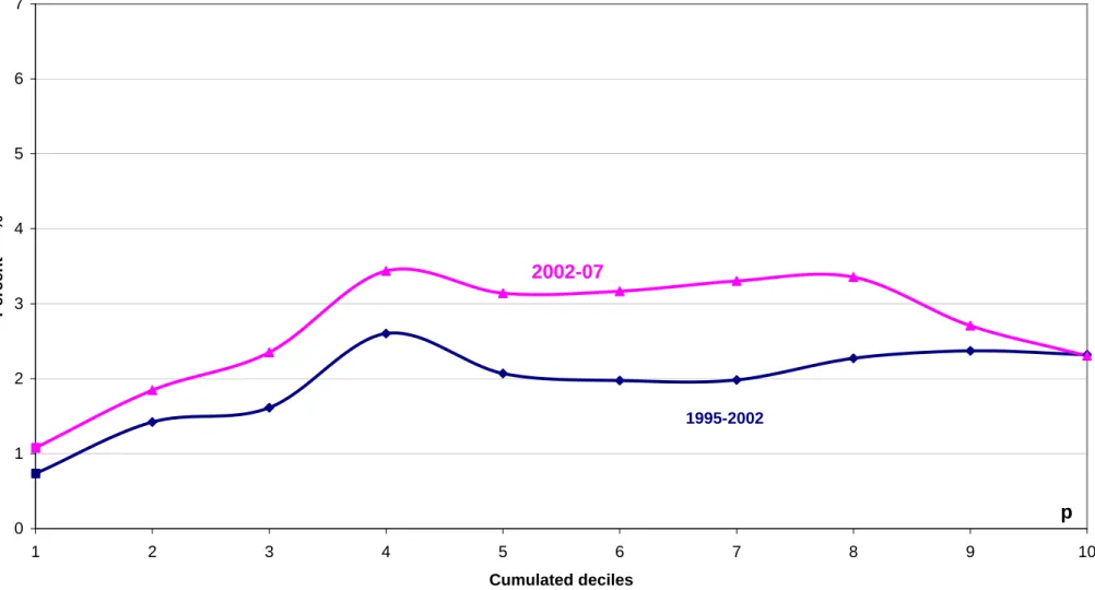
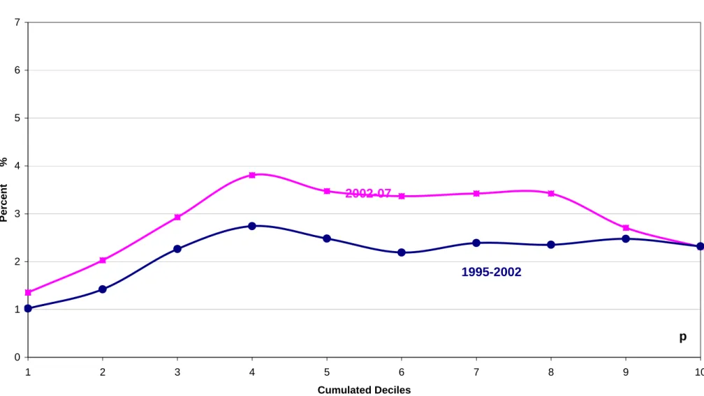
as-similated to GDP per capita. Data are drawn from the World Development Indicators (World Bank, 2009). Figure 1a shows the GIC curve of the global economy for the 1995-2002 period. To illustrate the comparison of growth paths discussed above, figure 1 also shows the GIC curve that would have been ob-tained for the same 1995-02 period had country growth rates over that period been those observed between 2002 and 2007. 4 _{It can be seen that there is no}

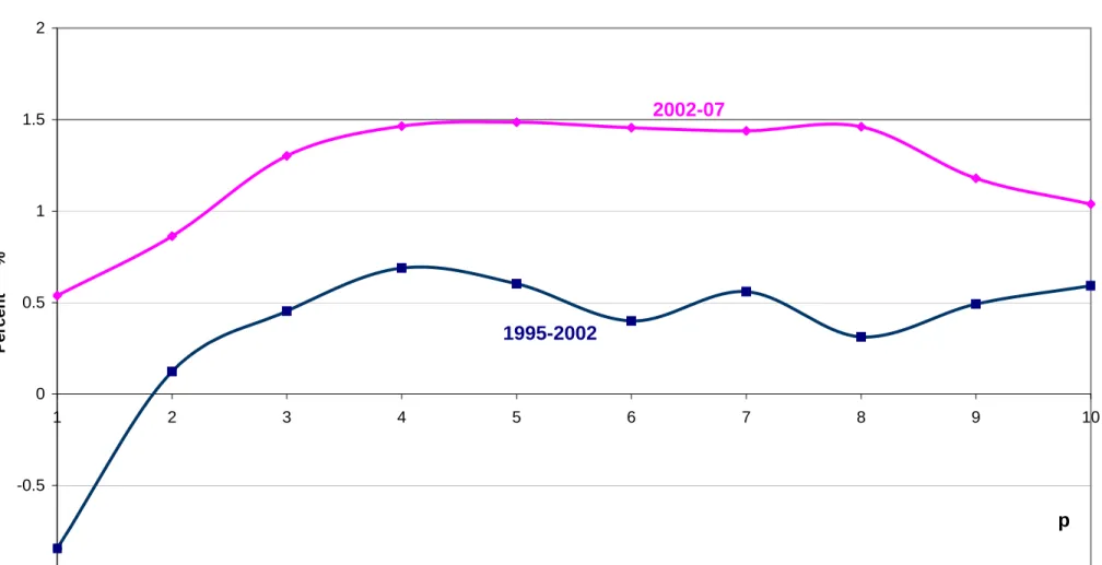
first order dominance because the mean income of the two upper deciles did not grow as fast in 2002-07 as in 1995-02. Figure 1b shows the p-cumulative growth incidence curves for the two periods. It can be checked there that second order dominance holds. In other words, social welfare would have been higher in 2002 with the 2002-07 growth rates than with the actual 1995-02 growth rates for all social welfare functions based on increasing and concave country income utility functions.

In the preceding example, it is important to stress that the comparison of two growth spells in the global economy is done using the same base year. Of course, it would be possible to define GICs for 1995-02 on the one hand and for 2002-07, using 2002 as initial year, on the other hand. Two remarks are in order in this respect. First, the shape of the 2002-07 GIC with 2002 as initial year is not the same as the 2002-07 GIC when 1995 is used as a base year as above - the 2002-07 growth rates being applied to 1995 country incomes. This is illustrated on Figure 2. Second, it must be clear that the F OD and SOD dominance results apply only when the initial distributions of the two growth paths being compared are the same. The GICs for 1995-02 and for 2002-07, with 2002 as a base year, can be compared but the comparison has little meaning in terms of social welfare.

3_{This is what Milanovic (2005) called ’inter-country’ rather than ’global’ distribution. Here}

we shall use the two terms interchangeably.

4_{In that comparison, the initial distribution is indeed the same -i.e. the 1995}

An ambiguity in interpreting GICs comes from the fact that the quantiles on the horizontal axis do not comprise the same statistical units. For instance, the 1995-02 GIC in figure 1a compares the mean income of the various deciles of the 1995 and 2002 distributions but the country composition of these deciles has changed during that time intervall. CICs thus are ’anonymous’ in the sense that the composition of the various quantiles of the distribution does not matter. For instance, Uganda and Tanzania moved out of the first decile whereas Eritrea and Madagascar moved in. If one is interested in whether global growth has been pro-poor between 1995 and 2002 there does not seem to be any good reason for ignoring what happened to countries that grew fast enough to move out of the bottom deciles.

An alternative to the GIC approach to the distributional features of growth consists of keeping the ranking of statistical units constant , whereas comparing the initial and terminal quantile functions , yF(p) and , yΦ(p), as done before is

equivalent to re-ranking them. The no-reranking approach to the distributional incidence of growth then associates to every quantile in the initial income dis-tribution yF(p) the terminal incomes Z(p) of individual units in that quantile.

The corresponding Growth Incidence Curve becomes ’non-anonymous’ since it it now possible to put a name on each point of the curve. Formally, non-anonymous Growth Incidence Curves (na-GIC)5 _{can be defined by:}

eg(p) = Ra

o zdeΦ(z | yF(p))

yF(p) − 1

In other words, the na-GIC associates to every quantile in the initial distribution the mean income growth of all individual units in that quantile. Likewise, the cumulative na-GIC curve may be defined as:

e G(p) = Rp 0_Reg(q)yF(q)dq p 0 yF(q)dq

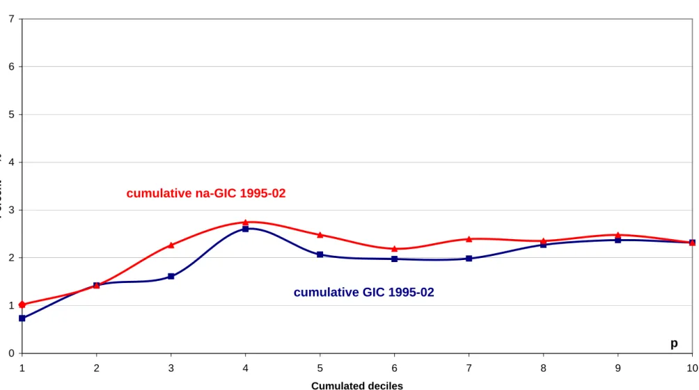
Figure 3a plots the modified GIC for the 1995-2002 gobal growth spell and compares it to the original GIC. The discrepancy between both curves is striking. The same is true of the cumulative modified and original GICs in figure 3b. In effect, the difference is such that comparing two different growth paths might well lead to different conclusions about their distributional impact depending on whether one does or does not re-rank the statistical units between the initial and the terminal year.The main differences between the GIC and the na-GIC in figure 3a comes from the fact that, between 1995 and 2002, India and Bosnia moved up from the third to the fourth decile of the distribution. The fast growth of these two countries is explicitly taken into account in the 3rd decile of the na-GIC whereas it is somewhat hidden in the change in the composition of the 3rd and 4th decile in the standard GIC.6

5_{Jenkins and van Kern (2008) and van Kern (2009) refer to the same curves as "mobility}

profiles".

It remains now to see whether the simple dominance criteria in comparing the standard GICs or cumulative GICs have some counterpart with na-GICs and whether they make any difference when comparing different growth paths.

3

The bi-dimensional approach: dominance

cri-teria when simultaneously accounting for

ini-tial and terminal incomes

As the preceding example shows the issue in evaluating the distributional impact of growth would seem to be whether the analysis must refer to the initial or the terminal situation of individuals or countries. If we are interested in pro-poor growth, should pro-poorness be measured comparing the poor in the initial and terminal distributions or should those individuals or countries that escaped poverty be taken into account? Interestingly enough, this issue is related to the length of the growth spell that is analyzed. In the preceding example, India was in the bottom three deciles of the global distribution in 1995. It is not anymore in 2002. Therefore, it is not included in the calculation of the mean growth rate of the bottom three deciles with the GIC approach. But, of course, it would have been included if the analysis had focused on a much shorter time period, say 1995-96. Ignoring the initial situation of observations therefore is equivalent with ignoring the time path between the initial and the terminal time of the period under analysis. This may be fine if the goal of the analysis is only to describe distributional changes between the initial and terminal points. It may not so if it is to evaluate social welfare along alternative growth paths.

This section considers the general case where social welfare depends on both initial and terminal incomes, or equivalently, initial income and income change. The case where social welfare depends solely on terminal income, which corre-sponds to the GIC approach, is a particular case of this general specification.

3.1

Decomposing the difference between two growth paths

into initial and transitional distribution differencesh

paths

Now that the analytical framework is explicilty bi-dimensional, it is possible to deal rigorously with the issue of comparing growth paths with different initial distrbutions. Consider then two growth paths described by the joint density

of the distributional effects of the 1997 crisis in Indonesia. The standard GIC curve suggests the crisis has been strongly regressive with poor people more severely affected than others, whereas the na-GIC for the same simulation data set points to the crisis being "progressive", initially poor people having done on average better tan the others.

functions of initial and terminal incomes: ω(y, z) and ω∗(y, z).One way or an-other, what matters is the difference between these two functions. With the same notations as above this can be written as:

∆ω(y, z) = ω(y, z) − ω∗(y, z). = f (y).e_{Φ(z | y) − f}∗(y).eΦ∗_{(z | y)} Then, a natural decomposition of that difference is:

∆ω(y, z) = f (y).∆e_{Φ(z | y) + .e}Φ∗_{(z | y)∆f(y)} (1) where ∆e_{Φ(z | y) = eΦ(z | y) − e}Φ∗_{(z | y) and ∆f(y) = f(y) − f}∗_(y).

A this stage, it is convenient to refer to ∆ω(y, z) as the difference in ’growth paths’ and to ∆e_{Φ(z | y) as the difference in ’growth processes’. The idea here is} that a growth path is the combination of a growth process -essentially a tran-sitional or conditional density function - with an initial distribution. The first part of ( 1) is the contribution to the difference in growth paths of the ’growth processes’, i.e. densities of terminal income conditional on intitial income. The second part is the contribution of the difference in initial distributions for a given growth process. To the extent that growth processes may be considered independently from initial distributions, then it is the first part of (1) that mat-ters. Hence the focus on growth paths with identical initial distributions in the preceding section, or the imposition of a given initial distribution for the comparison of two growth processes.

This choice of focusing on growth paths with identical initial distributions is important for social welfare comparisons. Considering simultaneously initial and terminal incomes within a social welfare dominance context can be done using the general bi-dimensional framework proposed by Atkinson and Bour-guignon ( 1982). But, if the point is to compare growth paths with the same initial distribution, then simpler and more powerful criteria derived in Atkin-son and Bourguignon (1986) can be used. The latter paper was referring to the comparison of two income distributions among households with different needs, the distribution of needs itself being constant. In the present context, that framework would be equivalent to replace ’needs’ by ’initial income..

In what follows, we briefly recall the results obtained in this latter paper, show how they apply to the present case and derive simple necessary conditions for dominance of one growth process over another that seem of practical use. Before doing this, however, some remarks are in order about the concept of social welfare dominance in two dimensions and the shape of social welfare functions to be used.

3.2

Defining welfare dominance among growth paths

Formally, the problem is to compare two growth processes given by the condi-tional distributions e_{Φ(z | y) and e}Φ∗_{(z | y) where z stand for terminal income} and y for initial income. The initial distribution of income is given by the cumu-lative density function F (y). Atkinson and Bourguignon (1982) suggested that

such comparison could be made by considering social welfare functions where individual utilities would depend on both initial and terminal income. This idea was analyzed further by Atkinson (1983) when analyzing mobility - assuming identical marginal distribution of terminal incomes too - and at a later stage by Dardanoni (1993) and Gottsshalk and Spolaore (2003) among others. Other authors had suggested to define social welfare on permanent incomes - see for instance Shorrocks (1978) or Chakravarty et al. (1985).7 _{The same perspective}

is adopted in what follows, except for the fact that, for analytical convenience, individual utility functions are specified as functions of initial income, y, and change in income, x (= z − y) with support [−a, a].

Let Ψ(x | y) and Ψ∗_{(x | y) be the corresponding conditional distributions}

over the growth processes being compared and

∆Ψ(x | y) = Ψ(x | y) − Ψ∗(x | y)

the difference between them. Denoting the utility an individual draws from his/her own growth process by u(y, x), the difference in overall social welfare between the two growth paths is defined as:

∆W = Z a

0

Z a

−au(y, x)d∆Ψ(x | y)dF (y)

(2) or, using quantile functions for the common marginal distribution F ():

∆W = Z 1

0

Z a

−au [y(p), x] d∆Ψ(x | y(p))dp

(3) Welfare dominance of growth process eΦ over eΦ∗_{holds in the sense of a family of}

utility functions, V , if ∆W ≥ 0 for all utility functions u( ) belonging to family V :

e

Φ%V Φe∗ ⇐⇒ ∆W ≥ 0 ∀u ∈ V

An interesting property readily apparent in (2) and (3) is that the dominance of a growth process over another in general depends on the initial distribution of income. It is thus posible that the growth process eΦ dominates the process e

Φ∗ for a given initial distribution F () but not for another.

3.3

Social welfare functions

Families of social welfare functions may be defined by restrictions imposed on the marginal utility of income change, x In effect, this is equivalent to imposing restrictions on the marginal utility of terminal income. Three families of func-tions will be considered depending on the number of restricfunc-tions imposed on the marginal utility of income change.

In the first family, V0, utility functions are only required to have positive

marginal utilities of income change:

V0= {u; ux≥ 0}

Nothe that no restriction is imposed on the marginal utility of initial income. This is because the two growth paths being compared have the same distribution of initial income so that no comparison has to be perfomed in that dimension. As no restriction is imposed on the way utility depends on initial income, this family of functions should lead to ’partial first order’ dominance’ relationships. A more restrictive family of social welfare functions requires the marginal utility of income change to decline with initial income. In other words, a drop in income is more painful the poorer people initially are and likewise an increase in income brings more additional utility the richer they are.

V1= {u; ux≥ 0, uxy≤ 0}

Although still no restriction is imposed on the marginal utility of initial income, this family of utility functions leads to the equivalent of first order dominance conditions in the uni-dimensional case because restrictions on utility functions are still limited to the first derivative of the utility function with repect to income change. To distinguish it from the previous case, it is conveninent to refer to dominance conditions defined by V1as ’full first-order dominance’.

Second order dominance may be obtained by imposing restrictions on the second derivative of utility with respect to income changes. In this respect, a sensible family of social welfare functions is:

V2= {u; ux≥ 0, uxx≥ 0, uxy≤ 0, uyxx≥ 0}

The marginal utility of income change is thus required to decline with the income change itself, a rather standard requirement, but this decline is supposed to be slower when initial income rises. The general intuition behind this is the same as for V1. It is essentially that utility depends less and less on income change as

initial income rises. The marginal utility of a given income change is lower for higer initial incomes in V1 (first order) and it declines more slowly with income

change in V2 (second order).

It must be noted that both families V1 and V2 include utility functions that

depend solely on terminal income, that is functions of the form: u(y, x) = h(y + x)

V1 requires functions h() to be increasing and concave, whereas V2 requires

in addition its third derivative to be positive. It can thus be said that dom-inance criteria based on V1 will necessarily be consistent with the standard

uni-dimensional dominance analysis where utility is assumed to depend solely on terminal income. However, V2 introduces the additional restriction that the

third derivative of h() must be positive.8 _{For the same reason, it can be said}

8_{In the uni-dimensional case, restrictions on the third derivatives of the utility functions}

are equivalent to the ’transsfer sensitivity’ axiom used by Shorrocks and Foster (1987) to generalize standard Lorenz dominance to cases where the Lorenz curves cross each other.

that both V1and V2are consistent with the well-known Pigou-Dalton principle,

but, of course add further restrictions to social welfare.

A much more general family of utility functions that belong to V1and V2 is

given by the following CES-like family of functions::

u(y, x) = [ayα+ b(y + x)α]β _{with α, β ∈ [0, 1] and a, b ≥ 0.} (4) Somehow, this functional form generalizes the standard permanent income hy-pothesis. In that expression, initial an terminal incomes are indeed substitutes but not necessarily perfect substitutes (case α = 1).

3.4

Dominance criteria

We now state the dominance criteria corresponding to the three preceding fam-ilies of social welfare functions.

3.4.1 Partial first-order dominance

Given the absence of any restriction on the way utility depends on initial in-come, the family of social welfare functions V0 simply leads to the standard

unidimensional first-order criterion for evey value of initial income. e

Φ%V0 Φe∗ ⇐⇒ ∆Wu≥ 0 ∀u ∈ V0 ⇐⇒ ∆Ψ(x | yF(p)) ≤ 0 ∀x, p (5)

3.4.2 Full first-order dominance

Applying directly the results in Atkinson and Bourguignon (1987) with a con-tinuous rather than a discrete specification for the dimension with the same marginal distribution leads to the following dominance condition.

e Φ % V1Φe∗ ⇐⇒ ∆Wu≥ 0 ∀u ∈ V1 ⇐⇒ (6) ∆Θ(x, p) = 1 p Z p 0 ∆Ψ(x | y F(q))dq ≤ 0 ∀x, p

In that expression, the function Θ(x, p) is simply the cumulative density func-tion of the income change x for the p smallest initial incomes, or the p-cumulative distribution function of the income change. This is the straight generalization of the first order dominance results in a single dimension to two dimensions. The partial first-order dominance criterion was leading to a comparison of the cumulative density fucntions of income change conditionally on initial income. The full first-order dominance criterion lead to the comparison of the cumulative density functions in both the income change and the initial income dimensions. It can be seen that full first-order dominance is less demanding that partial first-order dominance since it is now possible not to have dominance in the sense of (5) for some values of initial income but to have it in the sense of (6) when integrating along the initial income dimension.

3.4.3 Second-order dominance

The full first-order dominance criteria (6) is still very demanding since it requires the cumulative distribution function of one growth path to be everywhere below that of another. Intuitively, this property must certainly hold for low initial income levels and low income changes, but not so much for high levels of initial income or income changes. The second order dominance criterion based on the family V2 of welfare functions weakens that requirement by allowing cumulative

density functions of the growth paths being compared to cross each other. e

Φ % V2Φe∗ ⇐⇒ ∆Wu≥ 0 ∀u ∈ V2 ⇐⇒ (7)

∆H(x, p) = Z x

−a∆Θ(z, p)dz ≤ 0 ∀x ∈ [−a, a] and ∀p ∈ [0, 1]

In this expression H(x, p) is the integral of the cumulative function Θ(x, p) with respect to income change. It is well-known since Atkinson (1970) and Shorrocks (1983) that the conditions ∆H(x, p) ≤ 0 is strictly equivalent to Generalized Lorenz dominance. In the present case, given the fact that the income change may take negative values the concept of "incomplete change" is preferred to the generalized Lorenz curve. The following equivalence can easily be shown:

∆H(x, p) = Z x

−a∆Θ(z, p)dz ≤ 0 ∀x ∈ [−a, a] and ∀p ∈ [0, 1] ⇐⇒ (8)

X(q, p) ≥ X∗(q, p) ∀p, q ∈ [0, 1]

where X(q, p) (resp X∗(q, p)) is the income gain among the p poorest individ-uals in terms of initial income and, among them, the q poorest in terms of income change. X and X∗ _{are referred to as the ’p-cumulative incomplete}

in-come change’. The word ’incomplete’ refers here to the fact that only a fraction q among the p poorest are taken into acccount. Formally, it is given by:

X(q, p) =

Z Z(q,p) −a

zΘz(z, p)dz with Θ [Z(q, p), p] = q

and equivalently for X∗_{, where Θ}

z(z, p) is the density function of the distribution

of income changes for the p poorest in terms of initial income.

3.5

Some necessary conditions for dominance

Both (6) and (7) criteria compare manyfolds associated with growth paths. Dom-inance is achieved when one manyfold is everywhere above or below another. These manyfolds may not be very convenient to perform actual comparisons of growth paths, but it is always possible to restrict the comparison to a few values of p, q or x as done below in figure 5.

If this is found to be too cumbersome, it is still possible to focus on a few indirect indicators of the relative position of these manyfolds. Some interesting necessary conditions for dominance of one growth path over another can be derived in this way.

First, notice that by integrating below the Θ(x, p) manyfold, first order dominance requires that the p-cumulative mean income changes be higher on the dominating growth path for all values of p. This is also a requirement for second order dominance when considering the intersection of the X(q, p) manyfold with the q = 1 plane.

e

Φ ºV1 or V2 Φe∗ =⇒ X(1, p) ≥ X∗(1, p) ∀p ∈ [0, 1] (9)

This condition has a direct relationship with the na-GICs associated with eΦ and e

Φ∗_{as will be seen below.}

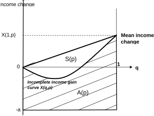
Second, integrating below the p-cumulative incomplete mean income change curves, X(q, p) with respect to q provides another necessary condition for second order dominance. Figure 4 shows the p-cumulative incomplete income change curve, X(q, p), for a given value of p. Integrating below this curve from the lower bound of income changes −a, one obtains an area with size A(p). The same could be done for the growth path eΦ∗ leading to an area of size A∗(p). If growth path eΦ dominates eΦ∗ _{in V}

2, then (8) implies that A(p) ≥ A∗(p) for all

p.

Another way of expressing this necessary condition for second order domi-nance of eΦ over eΦ∗_{is as follows. In figure 4 it can be seen that :}

A(p) = X(1, p)/2 + a − S(p) (10) where S(p) is the area between the bisector and the p-cumulative incomplete income change curve. Clearly, S(p) depends on the degree of inequality of the distribution of income changes. If they were all equal then the incomplete income change curve would simply be the bisector and S(p) would be 0. By analogy with the Gini coefficient, one can thus define an inequality index for the distribution of x as:

Γ(p) = 2.S(p)/X(1, p) (11) Combining (10) and (11) the necessary condition A(p) ≥ A∗_{(p) for the}

sec-ond order dominance of eΦ over eΦ∗becomes:

X(1, p) [1 − Γ(p)] ≥ X∗(1, p) [1 − Γ∗(p)] _{∀p ∈ [0, 1]} (12) According to (12)dominance of eΦ over eΦ∗_{requires not only that the}

p-cumulative mean income changes be higher for the dominating growth path but that this property still holds when mean income changes have been cor-rected by a term that takes into account the inequality in the distribution of income changes. One can thus refer to (12) as a condition on ’inequality-corrected p-cumulative mean income changes’.

A problem with this inequality corrected mean income change is that it may be negative. Indeed, it can be seen on figure 4 that the area S(p) may be larger than X(1, p)/2, which implies that the inequality coefficient Γ(p) may be larger than unity. This is essentially due to the fact that inequality is defined here on a variable that can take negative values. However, to the extent that what matters is the comparison between two growth processes, the sign of inequality corrected mean income changes may not be that important.

3.6

Dominance criteria and growth incidence curves

First, partial first-order dominance implies dominance of na-GIC curves. Noting x(p) and x∗(p) the income change means of the two growth paths for the pth_{quantile of the initial income distribution. The na-GIC curves are given}

respectively by x(p)/y(p) and x∗(p)/y(p). As partial first-order dominance (5) requires the conditional cdf of income change to be lower along the dominating growth path, this implies the income change means to be larger on that path:

e

Φ % V0Φe∗ ⇐⇒ ∆Ψ(x | yF(p)) ≤ 0 ∀x, p =⇒

eg(p) = x(p)/y(p) ≥ eg∗_{(p) = x}∗_{(p)/y(p) ∀p}

Second, both full-first-order and second-order dominance imply p-cumulative na-GIC dominance. This is the necessary condition (9) seen above. To extend that condition to p-cumulative na-GIC curves, it is only necessary to divide the p-cumulative income change means by the p-cumulative initial income means, Y (p) defined by:

Y (p) = Z p

0

yF(q)dq

The following implication then holds: e

Φ _º V1 or V2Φe∗ =⇒ X(1, p) ≥ X∗(1, p) ∀p ∈ [0, 1] =⇒

e

G(p) = X(1, p)/Y (p) ≥ eG∗(p) = X∗(1, p)/Y (p)

Third, second-order dominance leads to an extension of p-cumulative na-GIC curves that takes into account the inequality in the distribution of income changes. These inequality-corrected p-cumulative na-GIC curves, G(p), are de-fined by:

G(p) = e_{G(p). [1 − Γ(p).]} and the following implication holds:

e

Φ ºV2 Φe∗ =⇒ G(p) ≥ G

∗

(p)

Conceptually, this extension of na-GIc curves is important because it intro-duces a notion of ’income mobility’ or ’horizontal inequality’ into the description of the distributional features of growth. Standard GICs compare the distribu-tion of terminal income and thus refer implicitly to the change in vertical in-equality associated with growth. na-GICs account for income mobility but focus on mean income changes conditionally on initial income. Inequality-corrected na-GICs introduce horizontal inequality into the descriptyion of growth. Two growth paths may have the same p-cumulative na-GIC curves and quite dif-ferent inequality-corrected p-cumulative na-GIC curves, indicating that there is

more disparity in individual growth rates for given initial income in one path. That path could not dominate the other in the sense of V2.

A last point to be scrutinized is the relationship between the dominance criteria stated above and standard GICs. It has been seen that all families of social welfare functions defined on initial income and income change included social welfare functions defined on terminal income only. It should thus be the case that dominance criteria established in this section imply uni-dimensional dominance criteria which lie behind standard GICs.

This is easily checked. Consider for instance the partial first-order domi-nance criterion (5). The cumulative density function of terminal income, Φ(), associated with the conditional cdf of income changes Ψ(x | y) is given by:

Φ(z) =

1

Z

0

Ψ(x | y(p))dp

It follows that the partial first-order dominance criterion (5) implies first order dominance of the distribution of terminal income on growth path eΦ over path e

Φ∗. In turn this implies GIC dominance, i.e. gΦF(p) ≥ gΦ∗_F(p). The same

result can be proven for full first-order or second-order dominance. They imply dominance of cumulative GICs defined on terminal incomes.

4

An empirical illustration with the global

dis-tribution of income

To illustrate the preceding criteria, we use again the change in the global dis-tribution of income by country, comparing the 1995-02 period with what would have been the growth path if growth rates had been during that period what they have actually been between 2002 and 2007. Thus, the comparison between the two growth paths is made using the same initial income distribution as a reference, in accordance with a previous argument in this paper.

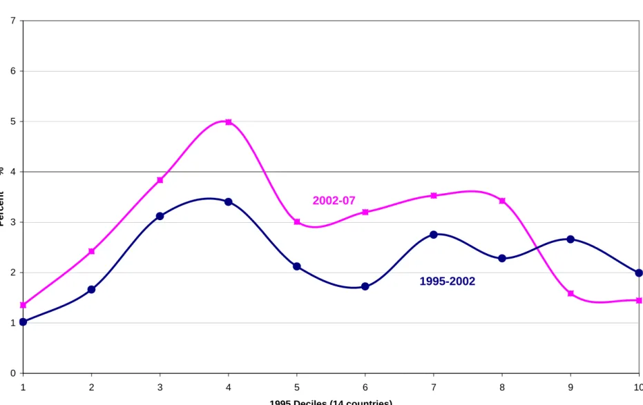
Figure 5 shows the na-GIC by 1995 income decile for the two growth processes. Despite the fact that the overall average growth rate has been larger in 2002-07, there is no partial first order dominance in the sense of (5), since the two curves in figure 5a cross each other. The annual growth rate in the 9th 1995 decile is lower along the 2002-07 growth path. On the basis of the p-cumulative na-GIC curves shown in figure 5b, there is no reason to reject full first order dominance in the sense of (6).

Moving now to second-order dominance in the sense of (7), figure 6 shows the projections of the incomplete income gain manyfold, X(q, p), on the q plane for selected values of p. For the ease of comparison with other charts, incomplete income gains are normalized by the mean 1995 income of the p deciles. So, the ordinate of the various curves at q = 100% for the various values of p corresponds to the mean income change shown on the p-cumulative na-GICs in figure 5b. Figure 6 suggests that second-order dominance holds. Indeed, the incomplete

income gain curves X(q, p) are everywhere higher for 2002-07 than for 1995-02, for all values of p being considered.

It logically follows from this that dominance must also hold for inequality-corrected p-cumulative na-GICs. Those curves are shown in figure 7 and this is indeed the case. Note on this figure that the inequality-corrected p-cumulative na-GIC is negative for the first decile of the distribution in 1995-02. In other words, the inequality coefficient, Γ(.1), turns out to be negative on that growth path, indicating a higher degree of inequality of gowth rates among the 10 per cent poorest countries according to 1995 incomes. In effect, it can be checked that the coefficient of variation of income gains is indeed lower for the poorest countries, as of 1995.

This example shows that the dominance criteria derived in the preceding section are not so restrictive as to prevent full dominance when comparing al-ternative growth paths for the global economy. Alal-ternatively, one may wonder whether the record mean growth rate observed during 2002-07 is not sufficient for dominance to hold whatever the country structure of growth behind that mean. The simple simulation reported in figure 8 shows that this is not the case.

The simulation consists of keeping the overall mean growth rate of the 2002-07 period constant while increasing the dispersion of growth rates across coun-tries. In effect, growth rates are artificially modified applying the following mean preserving spread rule:

gi → g + S(gi− g) + ui

where gi is the growth rate of country i, g the overall growth rate of the global

economy, S a scale factor arbitrarily set to 1.8 and uia corrective term ensuring

that full first-order dominance holds for the poorest countries while mean growth is preserved. This transformation is equivalent to increasing the inequality of income changes or growth-related income mobility. In other words, countries which initially (i.e. 1995) were close to each other in terms of income find them-selves more distant, and presumably at more distant ranks of the global income distribution in the terminal year of the period considered.

Figure 8b shows that the simulated 2002-07 growth path still dominates 1995-02 when considering p-cumulative na-GICs. However, figure 8c shows that dominance does not hold anymore when considering the inequality-corrected p-cumulative na-GICs. It follows that there cannot be dominance in terms of the incomplete income change (12) or the social welfare criterion (7).

This example illustrates the different meaning of the p-cumulative and the inequality corrected p-cumulative na-GICs. Even though these are only neces-sary conditions for dominance of a growth path over another, whether one is satisfied and the other is not gives some indication on the way the structure of growh affects overall dominance. If (9) holds and not (12) then the reason for no dominance is likely to come from more inequality in growth rates for initially close observations. In the opposite case, no dominance is more likely to be due to a lower overall mean growth rate. But, of course, a complete diagnosis can

only be obtained by considering the whole p-cumuative incomplete income gain curves, X(q, p).

5

Conclusion

This paper extended the concept of Growth Incidence Curve to that of non-anonymous Growth Incidence Curves where growth is evaluated for the various quantiles of the initial distribution of income without any re-ranking. This simple extension of the original growth incidence framework leads to considering simul-taneously initial and terminal incomes in evaluating growth, or equivalently to explicitly introducing income mobility into the description of the distributional features of growth.

The main contribution of this paper is to provide a rigorous bi-dimensional framework for the social welfare evaluation of growth, under the assumption that both terminal and initial incomes enter individual welfare. Bi-dimensional social welfare dominance criteria obtained in previous work have been adapted to this particular case and some interesting necessary conditions have been derived that compare growth processes on the basis of different definitions of non-anonymous growth incidence curves. Of special relevance is the ’inequality-corrected cumu-lative non-anonymous growth incidence curve’ where the mean income growth of the various quantiles of the initial distribution are scaled down by a factor that depends negatively on the degree of inequality of income changes within these quantiles. This simple dominance criterion thus takes into account changes in vertical inequality but also horizontal inequality, that is differences among people who are initially in the same situation.

Applying such criteria to evaluate growth clearly requires the availability of panel data on individual incomes. The empirical application in this paper relies on a particular panel which is the cross-country distribution of GDP per capita. It helped illustrating the various concepts being discussed, but it may be considered as too specific, especially in view of the fact that population weights were simply ignored. Other authors have worked on panel data of individual incomes in particular countries at various points of time and it might be interesting to study the properties of the instruments proposed in the present paper in this kind of framework.

Another field of application is the modeling of tax-benefit reforms. Typi-cally, the distributional aspects of these reforms are analyzed through ’micro-simulation’ techniques which simulate the income of every individual in a data base if a given reform were to be implemented. Comparing reforms with the help of the tools developed in this paper which allow combining vertical and horizontal inequality concerns seems promising.

6

References

Atkinson, A. (1970), On the measurement of inequality, Journal of Economic Theory, 2, 244-263

Atkinson, A. (1983), The measurement of economic mobility, in Atkinson, Social Mobility and Public Policy, Wheatsheaf books Ltd

Atkinson A. and F. Bourguignon (1982), The comparison of multi-dimensional distributions of economic status, The Review of Economic Studies, 54, 183-201

Atkinson, A. and F. Bourguignon (1987), Income distribution and differ-ences in needs, in G. Feiwel (ed), Arrow and the Foundations of the Theory of Economic Policy, Macmillan, London, 350-70.

Atkinson, A. ,F. Bourguignon and C. Morrisson (1992) Empirical Studies of Earnings Mobility, Harwood Academic Publishers

Benabou, R and E. Ok (2001), Mobility as progressivity: ranking income processes according to equality of opportunity, NBER Working Paper No. 8431 Chakravarty, S. , B. Dutta and J. Weymark (1985), Ethical indices of income mobility, Social CHoice and Welfare 2, 1-21

Dardanoni, V. (1993), Measuring social mobility, Journal of Economic The-ory, 61, 372-94

Fields, G. J. Leary and E. Ok (2001), The measurement of income mobil-ity: an introduction to the literature, in J. Silber (ed), Handbook on Income Inequality Measurement, Kluwer Academic Press

Fields, G. J. Leary and E. Ok (2002), Stochastic dominance in mobility analysis, Economics Letters, 75, 333-339

Fields, G (2009), Does income mobility equalize longer-term incomes? new measures of an old concept, Journal of Economic Inequality, Son; HH (2004), A note on Pro-Poor Growth, Economics Letters, 82(3), 307-14

Gottshalk, P. and E. Spolaore (2002), On the evaluation of economic mobil-ity, The Review of Economic Studies, 69, 191-208

Grimm, M. (2007), Removing the anonymity axiom in assessing pro-poor growth, Journal of Economic Inequality, 5(2), 179-197

Jenkins, S. and P. van Kern (2006), Terends in income inequality, pro-poor income growth and income mobility, Oxford Economic Papers, 58, 531-48

Lambert, P. (1993), The distribution and redistribution of income: a math-ematical analysis, Manchester University Press

Milanovic, B. (2005), Worlds Apart: Measuring International and Global Inequality , Princeton University Press

Ravallion, M. and S. Chen (2003), Measuring Pro-Poor Growth, Economics Letters, 78(1), 93-99

Ravallion, M. (2004) Pro-poor Growth: a Primer, World Bank Policy Re-search Working Paper 3242

Robilliard, A-S, F. Bourguignon and S. Robinson, Examining the social im-pact of the 1997 Indonesian crisis using a Macro-micro model, in F. Bour-guignon, L. Pereira da Silva and M. Bussolo (eds), The Impact of Macroeco-nomics Policies on Poverty and the Income Distribution, The World Bank and Palgrave

Shorrocks, A. (1978), Income inequality and income mobility, Journal of Economic Theory, 19, 376-93

Shorrocks A. (1983) Ranking income distributions. Economica 50:3-17 Shorrocks, A. and J.E. Foster (1987) ”Transfer Sensitive Inequality Mea-sures”, Review of Economic

Studies, 54, 485-497.

Son, Hyun Hwa (2004), A note on pro-poor growth, Economics Letters, 82, 307—31

Figure 1a. Growth Incidence Curve for global growth: average annual GDP per capita growth

rates by decile, 1995-02 vs. 2002-07 (using 1995 as base year)

0 1 2 3 4 5 6 7 1 2 3 4 5 6 7 8 9 10 Pe rc e n t % 1995-2002-07

Figure 1b. P-cumulative Growth Incidence Curve for global growth: average annual GDP

per capita growth rates for p poorest decile, 1995-02 vs. 2002-07

0 1 2 3 4 5 6 7 1 2 3 4 5 6 7 8 9 10 Percent % 1995-2002

2002-07

p

Figure 2. Global growth incidence curves: changing the base year of for 2002/07 growth

from 2002 to 1995 (annual rates)

0 1 2 3 4 5 6 7 1 2 3 4 5 6 7 8 9 10 Percent %

2002-07 (base 95)

2002-07 (base 02)

Figure 3a. Anonymous (standard) vs. Non-anonymous Growth Incidence Curves: global

growth, 1995-2002, annual rates

0 1 2 3 4 5 6 7 1 2 3 4 5 6 7 8 9 10 Percent %

GIC 1995-02

na-GIC 1995-02

Figure 3b. Anonymous (standard) vs. Non-anonymous p-Cumulative Growth Incidence

Curves: Global growth, 1995-2002, annual rates

0 1 2 3 4 5 6 7 1 2 3 4 5 6 7 8 9 10 Percent %

cumulative GIC 1995-02

cumulative na-GIC 1995-02

p

1

0

-a

q

Figure 4. p-cumulative incomplete mean income changes X(p,q) for given p

A(p)

Mean income

change

Income change

S(p)

X(1,p)

Incomplete income gain curve X(q,p)

Figure 5a. Non-anonymous Growth Incidence Curve for global growth: average annual

growth rates by 1995 decile, 1995-02 vs. 2002-07

0 1 2 3 4 5 6 7 1 2 3 4 5 6 7 8 9 10 Pe rc e n t % 1995-2002 2002-07

Figure 5b. Non-anonymous p-cumulative Growth Incidence Curve for global growth:

average annual growth rates for p poorest1995 deciles, 1995-02 vs. 2002-07

0 1 2 3 4 5 6 7 1 2 3 4 5 6 7 8 9 10 Percent %

1995-2002

2002-07

p

Figure 6. Projections of the p-cumulative incomplete income gain curve, X(q,p), on

the q plane (p=.3, .5,.8; 1): 1995-02 (solid lines); 2002-07 (dotted lines)

(income gains expressed as percentage of 1995 income)

-0.5 0 0.5 1 1.5 2 2.5 3 3.5 0 1 2 3 4 5 6 7 8 9 10 In co mp let e in co me g a in : % 1995 in co me in co me)

p = .3

p = .5

p = .8

p = 1

______

______

______

______

Figure 7. Inequality corrected non-anonymous p-cumulative Growth Incidence Curve for

global growth: 1995-02 vs. 2002-07

1995-2002

2002-07

p

Figure 8a. Non-anonymous Growth Incidence Curve for global growth: average annual

growth rates by 1995 decile: 1995-02 vs. modified 2002-07

0 1 2 3 4 5 6 7 8 1 2 3 4 5 6 7 8 9 10 Percent %

1995-2002

modified

2002-Figure 8b. Non-anonymous p-cumulative Growth Incidence Curve for global growth:

average annual growth rates for p poorest 1995 deciles, 1995-02 vs. modified 2002-07

0 1 2 3 4 5 6 7 1 2 3 4 5 6 7 8 9 10 Percent %

1995-2002

modified 2002-07

p

Figure 8c. Inequality corrected non-anonymous p-cumulative Growth Incidence Curve for

global growth: 1995-02 vs. modified 2002-07

-1 -0.5 0 0.5 1 1.5 2 1 2 3 4 5 6 7 8 9 10 Percent %

1995-2002

modified 2002-07

p