Geometric frustration: the case of triangular antiferromagnets

(1)

HAL Id: tel-00537747

https://tel.archives-ouvertes.fr/tel-00537747

Submitted on 19 Nov 2010

HAL is a multi-disciplinary open access archive for the deposit and dissemination of sci-entific research documents, whether they are pub-lished or not. The documents may come from teaching and research institutions in France or abroad, or from public or private research centers.

L’archive ouverte pluridisciplinaire HAL, est destinée au dépôt et à la diffusion de documents scientifiques de niveau recherche, publiés ou non, émanant des établissements d’enseignement et de recherche français ou étrangers, des laboratoires publics ou privés.

antiferromagnets

Pierre-Éric Melchy

To cite this version:

Pierre-Éric Melchy. Geometric frustration: the case of triangular antiferromagnets. Data Analysis, Statistics and Probability [physics.data-an]. Université de Grenoble, 2010. English. �tel-00537747�

(2)

THÈSE

thèse

Pour obtenir le titre de

de docteur de l’université de Grenoble

Spécialité : physique (matière condensée)

Arrêté ministériel : 7 août 2006 Présentée et soutenue publiquement par

Melchy Pierre-Éric

le 8 octobre 2010

Frustration géométrique:

le cas des antiferromagnétiques

triangulaires

Thèse dirigée par Mineev Vladimir et codirigée par Zhitomirsky Mike

jury

M. Holdsworth Peter

École Normale Supérieure de Lyon Rapporteur

M. Honecker Andreas

Université de Göttingen

Rapporteur

Mme Lacroix Claudine Institut Néel, CNRS

Présidente

(3)

(4)

i

Abstract

This doctoral dissertation presents a thorough determination of the phase diagrams of classical Heisenberg triangular antiferromagnet (HTAF) and its anisotropic variants based on theoretical and numerical analysis (Monte Carlo). At finite-field HTAF exhibits a non-trivial interplay of discrete Z3 symmetry and continuous S1 symmetry. They are successively broken

(discrete then continuous) with distinct features at low and high fields: in the latter case the ordering is along transverse direction; in the former case an intermediate collinear phase is stabilised before 120-degree structure is. Due to zero-field behaviour, transition lines close at (T, h) = (0, 0).

Single-ion anisotropy is here considered. Easy-axis HTAF for moderate anisotropy strength 0 < d 6 1.5 possesses Z6⊗S1symmetry at zero-field which induces triple BKT-like transitions.

At finite field the symmetry is the same as for HTAF: both thus share the same symmetry-breaking pattern. Yet specificities can be observed in the easy-axis system: splitting of zero-temperature transition at one-third magnetisation plateau, reduction of the saturation field.

Easy-plane HTAF belongs to the class of universality of XY triangular antiferromagnet: it thus interesting to start with this system. Zero-field behaviour results from the breaking of Z2 ⊗ S1 symmetry, where the discrete component is an emerging chiral symmetry. An

intermediate magnetically chiral ordered phase exists which extends to finite-field where the symmetry is Z2⊗Z3. The upper limit of this intermediate phase along field axis is a

multicrit-ical point at which transition lines are inverted. Above, the intermediate phase is a collinear phase. At high field the compound symmetry is broken as a whole Z6.

(5)

Résumé

Cette thèse de doctorat présente la détermination théorique et numérique (Monte Carlo) du diagramme de phase du système classique antiferromagnétique de Heisenberg sur réseau triangulaire (HAFT) et de ses variantes anisotropes. Sous champ HAFT présente une intri-cation non triviale des symétries discrète Z3 et continue S1. Elles sont successivement brisées (discrète puis continue) selon des modalités diﬀérentes à champ fort et modéré : dans ce cas-là l’ordre a lieu selon la direction transverse ; dans ce cas-ci une phase colinéaire intermédiaire est stabilisée avant la phase à 120 degrés. Du fait du comportement à champ nul les lignes de transitions se terminent à (T, h) = (0, 0).

L’anisotropie mono-ionique est ici considérée. HAFT avec anisotropie d’axe facile pour une anisotropie modérée, 0 < d 6 1.5, possède une symétrie Z6⊗ S1 à champ nul, qui induit

une triple transition BKT. Sous champ, la symétrie est identique à HAFT : les deux partagent donc le même scénario de brisure de symétries. Le système anisotrope présente toutefois des spéciﬁcités ; séparation de la transition à température nulle au champ de tiers d’aimantation, réduction du champ de saturation.

HAFT avec anisotropie de plan facile appartient à la classe d’universalité de XY AFT il est donc intéressant de commencer par ce système-ci. Le comportement à champ nul résulte de la symétrie Z2⊗ S1 où la composante discrète est une symétrie chirale émergente. Une phase

intermédiaire chirale magnétiquement désordonnée est stabilisée ; elle se prolonge sous champ, où la symétrie est réduite à Z2 ⊗ Z3, jusqu’à un point multicritique auquel les transitions

s’inversent. Au-dessus de celui-ci la phase intermédiaire est colinéaire. Sous champ fort la symétrie composite se brise comme une symétrie Z6 unique.

(6)

Acknowledgement

Preparing a doctorate couldn’t have been possible without the presence of many persons throughout the years as it is mere a certain achievement of a part of my life than a three-year challenging experience.

First I should thank my supervisor M. Zhitomirsky whose ruthless scientific demand prevented me to lean towards any kind of lazy thinking or lack of rigour. This is a rare quality in an inflating research world, quality for which I am really grateful to him. I’d also like to thank other senior researchers who were around during these years at CEA (thanked for its material support): J. Villain and V. Mineev for their mentoring and yet distant presence; X. Waintal, and M. Houzet for the fresh blood they are injecting into the theory group. As said there are many more persons who helped me along my way. Professors and tutors ignited and fueled my eager curiosity for understanding that has kept on growing with knowledge alongside an ever more acute perception of its stunning limitations requiring a tireless conquest of its frontier. In physics I’d like to thank F. Mila, B. Kumar, M. Kläui, P. Martin, A. Georges, M. Mézard, A. Aspect, J. Dalibard, J.-L. Basdevant, and S. Laurens. In mathematics I can’t help being grateful to J. Lannes, J. Chevallet, N. Tosel, and C. Viano. Other names arise in my mind from which I’d like to extract only two for this page not to turn into an endless tribute: J.-P. Dupuy for his enlightening conversations, for his passionate and yet rational to his fingertips commitment to the criticism of an erring science; S. Robert for his bright and reinvigorating approach to epistemology.

Beside these persons I cannot but warmly thank my colleagues turned friends and ﬁrst of all Raphaël who has shared much of the hard time and quite a few joyful moments of these last three years; Sean, who left a year ago, helped me a lot in many regards even though I may wish we had had more time to share ; Martin brought a cheerful and enthusiastic youth. Of course I met other so-called young researchers (PhD students and postdocs) whose encounter was appreciable: may they be thanked even without their naming. Yet I’d like to address personal thanks to a youngster whose passion for physics and joyful character brought quite an appreciable refreshment: Vincent.

For all their precious and enriching friendship throughout the years without which it would undoubtedly have been much harder if not impossible altogether I rejoice addressing with all my heart my very thanks to Claire, Delphine, Michel, Philippe,

(7)

Arnaud, Philippe, Jean-Paul, Arnaud, and François-Xavier. Their joyful warmth, their supportive presence, their challenging pieces of advice, their simple sharing the ups and downs are parts of what has helped me up. Persons I am profoundly grateful to and lovingly thankful to for their countless eﬀorts to foster my development, for their being inﬁnitely open-minded regarding my choices, wills and desires, for their never lacking support whatever the dire situation they, I, or we may be facing are my parents and my brother.

Last I’d like to thank these inspiring ﬁgures that enlighten my sky, all these great persons who make me proud of being called a human-being, whether they may be scientists, philosophers, artists or other great achievers, famous or not, of what can be called the best part of our humanity. Out of my personal sky I could name quite a few of these stars that lead my course. However I limit myself to the one who stood by my side throughout the writing of this dissertation and represents a model for any writer for his avoiding any superﬂuous note: Johann Sebastian Bach.

(8)

Chapter 1 Introduction

Condensed matter physics deals with matter in its condensed form: what does this tautology state? In this context condensed can be deﬁned as held together thanks

to internal interactions. It means that this branch of physics doesn’t investigate

el-ementary entities but the collective behaviour of interacting particles. Its name was coined rather recently (1967) by P. W. Anderson and V. Heine when they renamed their Solid-state Theory laboratory at Cambridge, UK, Theory of Condensed Matter. From a perspective in terms of macroscopic physical properties, they made the focus evolve towards the underpinning phenomenon, the grounding effect of which extends beyond the sole solid state, namely many-body interactions and the induced collective phenomena measurable either at a microscopic or macroscopic level. One of the most striking feature of collective phenomena is phase transition. Phase transitions are a commonly experienced fact — anybody cycling in winter does know that water in its solid form, also known as glaze when covering the ground, has quite distinct properties. Yet their understanding and their description is far less straightforward and has been fostering the development of theories and experiments by physicists for generations. They arise whenever there are competitive processes governing the equilibrium of a system: varying external parameters such as temperature, pressure, magnetic field, it is then possible to change the equilibrium configuration. The trouble in condensed matter physics stems from the hardship to analytically describe systems with more than two interacting particles: yet any realistic system such as this very sheet of paper consists of several billions of billions of atoms — this is no reason to conclude that this thesis is intractable: another important characteristic of condensed matter physics is to look at systems at the relevant scale and I doubt the atomistic one is the right choice for this piece of work! To overcome this hardship it has been necessary to develop ways of treating systems with a huge number of particles in a tractable way: this is what statistical mechanics can do. It makes use of the observation that physical properties of a given system can be correctly described by probabilistic distributions. Boltzmann can

(11)

without hesitation be named the father of this revolutionary approach.1 _{Thanks to this}

revolutionary viewpoint it has been possible to describe macroscopic properties of mat-ter from microscopic underpinning phenomena. The formalism of statistical mechanics, however originally devised in a classical language, could fully be extended to quantum context with a straightforward correspondence. With this toolbox in hand physicists could further develop the understanding of collective phenomena, among which critical phenomena that occur at phase transitions.

In a way or another various modern descriptions of critical phenomena are built upon the observation criticality is characterised by a loss of scale hierarchy: about phase transition the system look the same at diﬀerent scales — this auto-similarity is coined as fractal. In other words details don’t matter. An early understanding of this statement took the form of mean ﬁeld as enunciated by Weiss in 1907 [128]: this approach consists in considering for each particle the interactions with its neighbours and the environment at the level of mean values. However simplistic such a treatment may seem it has revealed not only fruitful to orientate intuitions but also exact in certain limits (roughly speaking in high dimensions for short-ranged interactions). Another development of this idea was proposed by Landau with his phenomenological description of second-order phase transitions2 _{based on a symmetry analysis of the system. Landau’s discussion is}

in fact two-fold. On the one hand he explicited symmetry rules governing a second-order phase transition: at a continuous transition there must be a group-subgroup relation between the symmetry groups of each phase on both sides of the transition. This leads to a classiﬁcation of possible continuous phase transitions given a model with a speciﬁc symmetry group. On the other hand he proposed an hydrodynamic-like development of the free energy functional in terms of successive powers of the order parameter and its gradient (which is possible at a continuous transition as the order parameter goes to zero3_{). Both sides of this reasoning work together as the development of the free}

energy functional introduces terms that must respect the symmetry of the model. This fruitful theory elegantly circumvents a major difficulty of statistical mechanics, namely the explicit calculation of partition function given a specific Hamiltonian. A later development fully pushing this idea of scale-invariance and discarding irrelevant details was the development during the 1960’s of renormalisation group by Kadanoff [41] and Wilson [129, 130]. The underlying idea is to describe the model at larger and larger

1

Boltzmann’s epitaph reads: S = k log W .

2

After Ehrenfest’s first classification of phase transitions according to continuity properties of the derivatives of free energy (in that classification an n-th order transition is a transition at which first discontinuity occurs for the n-th derivative), modern classification distinguishes first-order transitions characterised by the existence of non-zero latent heat from second-order ones that are continuous (without any latent heat) and associated with a diverging correlation length at the transition. Infinite-order transitions exist as well such as Berezinskii-Kosterlitz-Thouless transition that is dealt with in this dissertation.

3

Extensions of Landau’s formalism to certain first-order transitions can be done as presented for example in [119].

(12)

3 scales using a coarse-graining approach: during this transformation, that is called a flow, coupling constants of the model undergo changes that constitute a semi-group (hence the name that mathematically speaking is not exact) with certain constants flowing to zero, which means they don’t play any role for the criticality of the system. With this viewpoint it was then possible to introduce classes of universality: such a class groups various systems sharing common relevant interactions and consequently common symmetries. Each class can then be defined by a set of critical exponents that describe how quantities of interest such as specific heat behave in the vicinity of the transition. Most of physicists’ efforts in the analysis of phase transitions has thus been the determination of the class of universality which the model they investigate belongs to and in another direction the attempt to describe all possible classes of universality.

The latter eﬀort has undergone a dramatic change with conformal ﬁeld theory. This theory is based on the fact that critical theories are not only invariant under changes of scale as previously introduced with the renormalisation group but also under the action of conformal transformations4_{. If conformal invariance doesn’t bring anything}

new in dimensions d > 3, for d = 2 it does bring new constraints that should enable to catalogue bidimensional critical phenomena. This statement singles out the specificity of dimension 2. 2 d is in many regards specific as it offers a wealth of models with exotic critical behaviours that cannot be found in other dimensions; some of them even evade treatment with methods such as mean-field approximation, renormalisation group, and other methods perfectly working at higher dimensions. A way to grasp this specificity of bidimensional models is to think of their topological properties: as can readily be observed continuous deformations that are the pictorial way to glimpse at topology are far more restricted in 2d than in higher dimensions where it is often possible to circumvent a singularity using the extra dimensions. On the other side most methods used in 1d systems are specific to this dimension with the extreme constraint of the dimensionality that induces specific collective excitations.

Beside these theoretical achievements, numerical physics has grown in importance and played quite crucial a role in the understanding of critical phenomena. As pre-viously shortly alluded to one major hindrance in statistical mechanics is the actual handling of partition function. Numerical methods can precisely help overcoming it even without any explicit calculation of the partition function at stake — in the end the interesting elements are physical observables rather than mathematical devices used to built up theories. One major player in the ﬁeld of numerical statistical physics is Monte Carlo procedure in its various variants. Undoubtedly the algorithm proposed by Metropolis and coworkers [78] fostered the emergence of the ﬁeld, which has been fur-ther boosted by the exponential growth of computing facilities pushing furfur-ther away the balking limitations of numerical simulations. In a word the idea behind these methods

4

The group of conformal transformation is the subgroup of coordinate transformations that leave the metric invariant up to a scale factor, ie that preserve the angle between two vectors.

(13)

is to astutely explore the phase space to catch a faithful glimpse of the system under scrutiny: this is achieved through a Markov chain5_{. Numerics has thus grown as the}

third pillar on which modern statistical physics stands.

With this well equipped toolbox in hand it becomes possible to deal with phys-ical models among which magnetic systems constitute one of the most appreciated playground thanks to the variety of models that can be both theoretically devised and experimentally studied. An incomparable advantage of magnetic systems is in-deed that many experimental techniques are available to both probe macroscopic and microscopic properties: from bulk thermodynamical measurements (specific heat, sus-ceptibility, etc.) to local probing (atomic force microscopy, muon spin resonance), with such fine structural investigation tools as neutron scattering experiments (elastic and inelastic scattering, polarised or unpolarised neutrons, spin echo, etc.). Furthermore it is most of the time possible to write models accurately describing these spin systems or in the reverse way certain models initially theoretically devised and studied have proven relevant for the description of real compounds. For sure magnetic materials are less clean and less tunable than artificial magnetic crystals obtained in quantum optics. The latter are however still out of the energy range of interest and therefore remain promising experimental toys not yet at their full maturity [14].

As said condensed matter deals with collective phenomena and consequently coop-erative behaviours. In quite a few circumstances cooperation can lead to an extreme case which is frustration. Roughly speaking (more precise a definition is proposed in the following) frustration occurs whenever it is impossible for all interacting entities to simultaneously reach an optimum. In spin systems the concept was formally introduced in the 1970’s. With the rough picture above proposed it can readily be understood that this concept is relevant to a huge variety of problems in statistical mechanics, and even far beyond, as such fields as econophysics or sociophysics flourish. As previously pointed out magnetic systems provide an actual playground to deal with abstract concepts and frustration is no exception: various compounds indeed embody frustration and make it possible to confront models with experiments and reversely to seek inspiration in re-ality. Frustrated magnets offer quite an interesting playground to test various exciting concepts beside the release (or not) of frustration such as spin liquids, exotic phase transitions, quantum criticality, etc.

With this background in mind it is now possible to proceed to a more precise intro-duction of grounding concepts and questions supporting this dissertation. Symmetries in 2d is the topic of Sec. 1.1. Then a thorough introduction to frustration is proposed in Sec. 1.2. Last an historical perspective on the family that models studied in the fol-lowing chapters of this dissertation belongs to, namely antiferromagnetic spin sytems on a triangular lattice, is proposed in Sec. 1.3.

5

A Markov chain is a random process such that next step only depends on the current state: it is memoryless, which makes it perfectly suited for numerical simulations.

(14)

1.1. SYMMETRY BREAKING IN2D 5

1.1 Symmetry breaking in 2d

When dealing with phase transitions in general the question of symmetry breaking naturally comes out. In 2d this issue acquires a dramatic specificity. In 1966 Mermin and Wagner demonstrated that the breaking of a continuous symmetry in bidimen-sional systems is impossible at any finite temperature. As a consequence second-order phase transition in spin systems with continuous rotational symmetry, as is the case of isotropic models of spins with more than one component in zero field, is excluded. This statement doesn’t end the story. Berezinskii on the one hand [10, 11], Kosterlitz and Thouless on the other hand [61] argued that despite its continuous symmetry XY model on the square lattice does undergo a finite-temperature transition. No symmetry-breaking is associated with this transition but a dramatic change in the behaviour of stable topological defects. Such a transition is an example of an infinite-order transi-tion; this one is referred to as a BKT transition. The discussion of phase transition in terms of topological defects was formalised by different physicists [82, 76, 75, 79] in the late 1970’s. It is based on homotopy groups: these groups concentrate the sufficient information to describe topological properties of objects. The simplest one, the fun-damental group, π1, describes how closed loops in a topological object evolve under a

continuous deformation. For example any closed loop on the sphere S2 _{can be shrunk}

to a point, hence the fundamental group of the sphere is the trivial group: π1(S2) = 0.

On a circle the situation is less simplistic: some closed loops can twine around the cir-cle without being shrinkable to a single point; moreover these can twine several time, which means an integer can be associated to loops which is its winding number (zero in case of a shrinkable loop). This makes it understandable that the fundamental group of a circle is the group of integers: π1(S1) = Z. This theory enables the handling

of topological defects which exist in physical systems. These topological defects can induce phase transitions, which means it is possible to describe phase transition cal-culating the homotopy group of the symmetry group of the Hamiltonian. XY model exempliﬁes this approach: the symmetry group of the Hamiltonian is S1_{; as seen above} π1(S1) = Z. As a consequence XY system admits stable point defects that are integer

vortices. The observation put forward by Berezinskii, Kosterlitz, and Thouless is that vortices are bound into pairs of vortex-antivortex at low temperature and are free at high temperature, which means a transition occurs in between: this binding-unbinding transition is BKT transition. As a consequence of above mentioned Mermin-Wagner theorem the order settling below the transition is not a long-range order but rather a quasi-long-range order. This low-temperature phase is hence a soft massless phase with power-law decaying correlation functions and continuously varying critical exponents in contrast to what happens in Ising model with its massive low-temperature phase.

An interesting question is then the evolution from one model to the other. A way to study it consists in investigating discrete Abelian models with Zp symmetry. Beside

(15)

bidimensional crystals that are governed by discrete rotational symmetry (p = 2, 3, 4, 6 are of experimental relevance). If an XY model perturbed by Zp terms was studied by

José and coworkers in their seminal 1977’s work, ﬁrst speciﬁc studies of pure Zp systems

came slightly later [28, 17, 27]. These works showed that there is a critical value pc

such that for p 6 pc two massive phases exist as in Ising model whereas for p > pc

between these two massive phases an intermediate critical massless phase (or quasiliq-uid) emerges the lower limit of which tends to zero as p goes to inﬁnity in agreement with Mermin-Wagner prescription. An even more striking result has been obtained on p-state clock model, aka Zp models: the existence of an extended universality [65].

Above a certain temperature Teu for p > 4, thermodynamical properties are proved

identical to those of the continuous model p = ∞. In particular for p > 8 this collapse starts in the intermediate quasiliquid phase, which implies that the upper transition is a real BKT transition. It constitutes an example of an emergent symmetry.

Another example of an emergent symmetry in bidimensional systems is the one of an extra discrete degeneracy in certain bidimensional systems with a continuous symmetry [122]. This phenomenon revealed by Villain arises as a consequence of multi-q structure. Let’s introduce a spin structure Si = u cos q·ri+v sin q·riwhere u and v are orthogonal

unit vectors and q is an ordering vector6_{. In case this structure describes all ground}

states, which is the case with spins of dimension n = 2 or 3 (unless the ordering vector

q lies at special positions within Brillouin zone in this latter case), this formula shows

that an extra discrete degeneracy exists for spins of dimensionality n = 2 as soon as the star7 _{of q consists in more than one vector and for n > 3 if the star is not reduced to} {q, −q}. Let’s explicit this assertion in the former case: changing q into −q changes

sine into its opposite.As the vectors are bidimensional there is no direct continuous transformation to change q structure into −q structure. The existence of this extra degeneracy makes it possible for the system to order at ﬁnite temperature despite its original continuous symmetry. A widely discussed example is the case of XY model on the triangular lattice with its emergent chiral order that is presented in Chap. 4.

1.2 Frustration

Frustration is a concept that was formally introduced in the context of spin glasses [121, 123] even though earlier studies dealing with frustrated magnets exist [125, 114, 44, 2]. A characteristic property of frustrated systems, namely their extensive entropy at zero temperature, was discussed as early as 1935 by Pauling [96] in water ice. Frus-tration can be deﬁned as the impossibility to minimise all individual interaction terms

6

qis obtained as a vector minimising with respect to k the Fourier transform PjJijcos k · (ri− rj)

where (Jij) is the set of bilinear exchange constants defining the Hamiltonian H = PhijiSi· Sj.

7

The star of a vector k is the set of inequivalent vectors generated by the action of the lattice symmetry group on the vector k.

(16)

1.2. FRUSTRATION 7

at the same time, may it be due to randomness, to geometric constraints, or to com-peting interactions. After the formal introduction of the term frustration, frustrated magnets without randomness were studied for a while for their connection with spin glass. Yet it soon became obvious that these magnetic systems that had been stud-ied for some of them before the hype about spin glass could bring more. Thanks to the diversity of experimental methods available to study magnetic systems, this field of research has experienced a continual and vivid cross-fertilisation between theoreti-cians and experimentalists. Investigations on frustrated magnetic materials have had implications far beyond magnetism itself. Indeed their highly degenerate ground state manifold, their possibly non-collinear or incommensurate order, the assumptive spin liquid, and their possibly novel phase transitions offer a playground to investigate chal-lenging and exciting fundamental questions both in classical and quantum systems. Regarding quantum systems such questions as the link between cuprates supraconduc-tors and 2d quantum frustrated antiferromagnets [3] or as deconfined quantum critical point, which is a new paradigm to describe phase transitions beyond Landau-Ginzburg-Wilson paradigm encompassing transitions between phases with no symmetry relation [104, 105], have renewed the vivacity of research on this topic. Interestingly various analytical, numerical and experimental techniques have been used to study frustrated magnetic systems: analytical developments à la Onsager, Landau-Ginzburg treatment and more generally analysis of symmetry and topological properties, mean-field tech-niques, renormalisation group apparatus, high- and low-T series expansions, Monte Carlo simulations, experimental investigations. In certain cases some of these differ-ent approaches may be at odds such as exemplified by the opposition between certain renormalisation group methods (ε = d − 2 development of a non-linear σ model) on the one hand and Monte Carlo simulations and topological discussions on the other hand to describe classical frustrated Heisenberg spin systems [4, 49]. Renormalisation group approaches, Monte Carlo simulations and experimental measurement do not yield a consistent picture of such systems, which is the illustration how non-trivial the critical behaviour of frustrated magnets is. It also points out the necessity to carefully under-stand the limitations of the techniques that are used in order to identify the origin of such mismatches; hence a better insight into these techniques can be gained. Frustrated magnetism has been at the heart of much highlighted research of the past thirty years as is the case with cuprates high-Tc supraconductors, Josephson junction arrays,

multi-ferroics, etc. The most recent topic creating a real hype in this ﬁeld was the description of pseudo magnetic monopoles in spin ice systems [18]. Frustration can be studied in insulating crystals as well as in metals or in disordered systems. Hereafter we consider only the case of insulating crystals.

In insulating crystals the relevant picture to understand magnetism is the one of isolated spins located at vertices of a lattice. From the Hubbard model one can derive localised-spin interaction Hamiltonians: depending on spin dimensionality, they are Ising (1d spin space), XY (2d) or Heisenberg (3d) models. The simplest cases consist

(17)

in bilinear interaction terms. In such cases the competition of interactions inducing magnetic frustration can stem either from a competition between diﬀerent interaction paths (typically between nearest-neighbours and next-nearest neighbours) or from the topology of the lattice. Widely studied examples of the former case are J1− J2 model

on the square lattice, spin ladders, among others [21, 81]. In the latter case the frus-tration is said to be geometric. Geometrically frustrated magnets build up a major and diverse group of magnets. Geometrically frustrated systems can typically be built with triangular elementary plaquettes that can arrange either on a corner sharing pattern (kagome lattice) or on an edge sharing one (triangular lattice), in 2d or 3d as well. Another common building block is tetrahedron (corner sharing tetrahedra can form the so-called pyrochlore lattice). Common frustrated lattices comprise the 2d triangular lattice, kagome lattice, fcc, and pyrochlore among other ones. Numerous materials in this class exist [36]: anhydrous alum, jarosites, pyrochlores, spinels, magnetoplumbites, garnets,etc. Geometrically frustrated spin systems enable us to study frustration in very simply formulated models and to deal with non-trivial topology questions. Indeed an important characteristic of these systems is the nature of the order parameter which can be such an object as a matrix of SO(3), or a complex vector with S1 _{⊗ Z}

3

sym-metry group. Homotopy theory then yields non-trivial topological excitations, which may lead to exotic phase transitions. The identification of a new class of universality is however a tricky issue due to the non-trivial critical behaviour of frustrated spin sys-tems and the complicated order parameter symmetry group. A famous example of such a difficulty is provided by the twenty-year-long controversy about the nature of the phase transition in Heisenberg antiferromagnet in stacked triangular crystals. Early claims of a new universality class based on two-loop renormalisation group analysis and Monte Carlo simulations appeared [47, 48]. Various simulations and theoretical analysis were then published. Using a non-linear σ model Azaria and coworkers [5] claimed the transition should pertain to O(4) universality class if it were not first-order or mean-field tricritical. Tissier and coworkers published an extensive non-perturbative renormalisation group study of frustrated spin systems in dimension between two and three: a consequence of their study is that the transition of Heisenberg stacked trian-gular antiferromagnet is first-order; they further argue that the reason why numerical simulations stalled around the transition and identified it as second-order with new critical exponent is the existence of a region in the flow diagram where the flow is slow, inducing a very weak first-order character [116, 118]. Last Ngo and Diep published a careful Monte Carlo simulation using both advanced techniques and very large clusters to support the first-order character of the transition [88]. Similarly in this work we present results that firmly stand against a new universality class for the breaking of

S1 _{⊗ Z}

2, which agree with the detailed analysis presented on fully frustrated XY spin

systems [37].

An important characteristic of frustrated magnets is the extensive degeneracy of low-energy modes, which induces extensive entropy at zero temperature. Such a highly

(18)

1.3. TRIANGULAR ANTIFERROMAGNET: HISTORICAL PERSPECTIVE 9

degenerate ground state manifold can induce some long sought states such as spin liquids or spin glasses without any randomness, which is another reason why so much effort has flowed into research on frustrated spin systems. Spin liquids can be defined as gapped spin systems with a finite correlation length at zero temperature [80]. One good example of this is kagome antiferromagnet; yet its experimental realisation is still lacking: the grail of a perfect spin-1/2 kagome system still seems far away. A dramatic consequence of such a degeneracy is the possible appearance of extra soft modes, at least at T = 0 as is the case for XY classical spins on the triangular lattice or for Heisenberg spins on the triangular lattice. This is however a fragile feature that is quite sensitive to various perturbations and makes it even harder to observe, all the harder as an order by disorder phenomenon [124], for example induced by thermal fluctuations, can occur. It is by no way a systematic phenomenon in geometrically frustrated systems as Heisenberg pyrochlore and four-component spin system on kagome lattice show: both remain disordered at low temperature [86].

Yet ways to remove this accidental continuous degeneracy exist. First, thermal ﬂuctuations are expected to induce an order by disorder phenomenon as pointed out by Villain and collaborators at the very beginning of 1980’s [124]; however such an ordering may occur in certain cases only at higher order than the second one as discussed by Sheng and Henley [106]. Quantum ﬂuctuations are another way to reduce degeneracy and induce order that will not be developped in this work. Last anisotropy changes symmetry, which may induce ordering: this point is the object of a large part of the work here presented.

1.3 Triangular antiferromagnet: historical

perspec-tive

When considering geometric frustration the simpler system to come to the mind is an antiferromagnetic model on the triangular lattice. With their stunning simplicity triangular antiferromagnets have been occupying physicists for several decades. As this dissertation deals with classical systems the historical perspective here proposed leans towards classical systems even though their quantum counterparts do present several interesting features. Reviewing what has been done on triangular antiferromagnets clearly shows various research on these systems have gone diﬀerent paths. After the historical exact solution of Ising models [125, 126] completed by the demonstration this model belongs to Ising universality class with a Z6 symmetry-breaking term [1] with an

upper transition at T = 0 and further reﬁnements in the discussion of Z6

symmetry-breaking as reinforced by the introduction of next-nearest-neighbour couplings [63, 33], much effort has been devoted either to quantum Ising models with and without field (in the latter case, a transverse field enables to have a glimpse at other interesting models: the dual model is a Z2 gauge model that is equivalent to quantum kagome

(19)

antiferro-magnet, system expected to exhibit a spin-liquid phase) or to stacked triangular Ising antiferromagnet. The investigation of stacked triangular antiferromagnets in case of

XY and Heisenberg models has also gathered much attention, probably thanks to

ex-perimental realisations of these models [23, 49]. Most investigated layered compounds diverge from 2d models as they are in fact chains weakly coupled in a triangular lattice, and thus exhibit 3d ordering properties of quasi-1d objects. A large class of compounds pertains to ABX3 family where A stands for Cs or Rb, B for a magnetic ion, either

Mn, Cu, Ni, or Co, and X for one of the halogens, Cl, Br, or I. Depending on the kind of anisotropy in the compound relevant model changes. For those with a strong easy-axis anisotropy Ising model is adapted: this is the case of CsNiCl3, CsNiBr3, and

CsMnI3. Easy-plane anisotropy as present in CsMnBr3 and CsVBr3 leads to a

descrip-tion with XY model. As for systems with a very weak anisotropy, such as CsVBr3

and RbNiCl3, they let Heisenberg model correctly describe them. Another reason why

stacked systems have been so widely studied is their amenability to mean-field analysis [97, 99, 101, 100]. As already discussed a twenty-year-long controversy opposed propo-nents of a continuous transition from the paramagnetic to the ordered phase in XY and in Heisenberg stacked triangular antiferromagnet to opponents claiming these transi-tions were first-order. After the non-perturbative renormalisation group approach by Tissier and coworkers [116, 118, 117], and various numerical treatment, Ngo and Diep proposed clear numerical evidence of a first-order transition thanks to Wang-Landau flat histogram algorithm implemented on quite large clusters [89, 88] (and references therein for previous numerical works).

At the other end research on 2d models and quasi-2d compounds has generated fewer publications, many extensively discussing zero-field behaviour. The work by Miyashita and Shiba on the one hand [85] and by Lee and coworkers on the other hand [66, 67] really started the investigations on 2d XY model which were complemented by Kawa-mura’s spin-wave calculations [46] and Korshunov’s extensive analysis of symmetry and topological excitations [57, 56, 60, 59]. The interest rose due to the emergent chiral tran-sition as already forecast by Villain [122]. As a consequence two symmetry-breaking occur, which at zero-field induces two distinct transitions that some authors failed to distinguish [66, 67] as opposed to others [85, 68, 134, 69, 91]. Yet finite-field behaviour has lacked thorough careful investigations despite the quite fine discussion proposed by Korshunov [57], which was a motivation to undertake such investigations. As far as Heisenberg triangular antiferromagnet is concerned if its quantum version has been rather popular the classical model has been only quite partially studied. Zero-field be-haviour, after the pioneering and inspiring topological analysis proposed by Kawamura and Miyashita [51, 50], did attract some interest [5, 6, 109, 133, 132, 53]. As this model has a continuous symmetry in zero-field, after Mermin-Wagner theorem it is expected no finite-temperature transition can occur. Kawamura and Miyashita challenged this view putting forward the existence of two regimes with distinct properties of the stable point topological defects, namely Z2 vortices. Further numerical achievements [53] and

(20)

1.3. TRIANGULAR ANTIFERROMAGNET: HISTORICAL PERSPECTIVE 11

an experimental realisation of an Heisenberg triangular antiferromagnet [87] propose convincing support for this transition. Finite-ﬁeld behaviour contrastingly has been at best overlooked [52]. With so little theoretical work on it and with new experimental results on quasi-2d compounds (Rb4Mn(MoO4)3, Nakatsuji et al., private

communica-tion) did require a correct study.

In this context the work presented in this dissertation intends to propose a clear picture on the whole phase diagram of classical Heisenberg model (Chap. 2) and its anisotropic variants, namely easy-axis (Chap. 3) and easy-plane anisotropic models (Chap. 4) based on a blend of numerical simulations and symmetry analysis without any heavy technical apparatus. If studies were published presenting elements of a phase diagram for anisotropic models [84, 83], the anisotropy was exchange anisotropy. From an experimental point of view single-ion anisotropy as used here seems more relevant. Furthermore from a theoretical point of view its perturbing impact is much more dra-matic. As easy-plane anisotropic Heisenberg triangular antiferromagnet is presented and since a precise phase diagram was still absent, XY triangular antiferromagnet has been studied as well and results are presented in Chap. 4.

(21)

(22)

Chapter 2 Heisenberg Triangular

Antiferromagnet

In this chapter we deal with the isotropic version of Heisenberg triangular antiferro-magnet (HTAF); in a way this is the original version that is referred to when speaking of Heisenberg antiferromagnetic model on the triangular lattice. In the first section the model is briefly introduced and key properties of its Hamiltonian are exposed. Then results on zero-field behaviour are reviewed and critically compared. Sec. 2.3 and 2.4 are devoted to finite-field behaviour: first we discuss symmetries of HTAF in an exter-nal field, then our numerical calculations for this system are presented and the phase diagram of HTAF proposed. Considering existing results on zero-field behaviour of HTAF, a new study has seemed worthless; yet to support this viewpoint and to draw a complete picture of the phase diagram of HTAF as here intended, a critical review of literature on this topic is included.

2.1 Model

To deal with electronic crystalline systems it is necessary to take into account two competing energies describing the behaviour of electrons: Coulomb repulsion and ki-netic energy (hopping). If the incompletely ﬁlled orbitals (3d in iron-group elements and 4f in rare-earth elements) are decribed by localised orbitals, this is encompassed in so-called Hubbard model:

H = X n,n′_,s bn′_−na†_n′_,san,s+ U X n a†_n,↑a_n,↑a†_n,↓a_n,↓ (2.1)

where n indexes sites and s is a spin index, a†

n′_,s a fermionic creation operator creating

an electron at site n with spin s and an,s the associated annihilation operator.

(23)

This Hamiltonian can be written in another form when developing it in the low-energy sector:

H = JX

hi,ji

Si· Sj (2.2)

where I have assumed for simplicity symmetry in the bn′_−n terms and then a single

exchange energy (J can indeed be written in terms of an exchange integral). This Hamiltonian is called Heisenberg Hamiltonian [136]. When considering systems with large spins it is quite appropriate to describe spins as classical vectors which makes Heisenberg model more tractable. In systems for which this work is relevant such an approximation is correct (most of them are rare-earth compounds) and from now on only classical models are used unless otherwise stated. For simplicity classical spins are normalised to one.

Hereafter we consider HTAF with an applied ﬁeld:

H = X hi,ji Si· Sj − h · X i Si (2.3)

written in the units of the exchange constant J. Even though we did not specifically work on zero-field behaviour a glimpse on what happens without any field will be given for the phase diagram to be entirely discussed.

Let’s discuss the ground states of (2.3) first at zero field then at finite field. A preliminary observation is the following transformation of (2.3):

H = 1₂X ∆ (S∆,1· S∆,2 + S∆,2 · S∆,3+ S∆,3· S∆,1) + h 6 X ∆,i S∆,i (2.4) = 1 4 X ∆ Ç S∆,1+ S∆,2 + S∆,3 − h 3 å2 + const. (2.5)

where summation runs over triangular plaquettes ∆.

This transformation makes it plain that to minimise the Hamiltonian a sufficient condition is to equate each square in the sum to zero, which is possible: it even makes it obvious that imposing a specific structure on a given triangle imposes the config-uration on the whole lattice. Let’s indeed consider a given triangle ∆: let’s pick up one configuration satisfying S∆,1+ S∆,2+ S∆,3 = 0 (infinity of solutions, among which

those with spins pointing at 120 degrees from one another equally share frustration on the three bonds); then on a neighbouring triangle ∆′ _{there is a unique solution to}

S∆′_,1+ S_∆′_,2+ S_∆′_,3 = 0 as the two spins pertaining to both ∆ and ∆′ are already ﬁxed,

qed. As a consequence ground states respect a three-sublattice pattern, the so-called

√

3×√3 pattern that is associated with ordering wave vector q0 = (4π/3, 0). Obviously

the condition is a necessary one as well: if one of the squares in the sum were non-zero then the energy of the considered configuration would be strictly larger than the one of configurations with all squares equal to zero – these configurations exist as already

(24)

2.2. BRIEF REVIEW OF ZERO-FIELD BEHAVIOUR 15

demonstrated – and hence would not be a ground state, qed. Such a constraint how-ever lets a continuous degeneracy appear in the system. There are indeed six degrees of freedom corresponding to the three unit-length vectors (spins) constrained by three equations: three free parameters remain. A closer look at this extra degeneracy shows that it corresponds to the degrees of freedom of the three-spin structure on a triangular plaquette, thence the corresponding order parameter space SO(3).

As previously discussed the ordering respects a three-sublattice pattern: it is thus natural to describe the spin structure as:

hSii = l1cos(q0· ri) + l2sin(q0· ri) + m (2.6)

where m is static magnetisation, which is zero at zero ﬁeld, and l1 and l2 are

antiferro-magnetic ordering vectors. In this language, 120-degree structure corresponds to a pair of orthogonal vectors l1 ⊥ l2, |l1| = |l2| and m = 0. In case of a distorted 120-degree

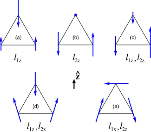
structure (either due to field or easy-axis anisotropy) m 6= 0. Let’s present two other configurations of importance as well (an overall view of low-field planar configurations can be found in Fig. 3.1). Collinear fully-ordered configuration, so-called up-up-down configuration, is characterised by l2 = 0 and l1 and m collinear. High-field planar

V-shape configuration is defined by l2 = 0, l1 having components both along the field and

transverse to it, and m along the applied ﬁeld direction.

2.2 Brief review of zero-field behaviour

At zero field this extra continuous degeneracy of ground state manifold coincides with order parameter space which is SO(3) the group of rotations in 3 dimensions, or in a more pictorial language the rigid body of three spins in a given triangle. Let’s discuss possible phase transitions in such an order parameter space. First, an important remark should be put forward: in this two-dimensional system there cannot be any finite-temperature phase transition associated with the breaking of a continuous symmetry, after Mermin-Wagner theorem [77]. With this viewpoint there shouldn’t be any finite-temperature transition in HTAF. However the conclusion becomes less obvious when the question is dealt with from a topological viewpoint: indeed stable topological defects exist in HTAF, which may induce a phase transition in a similar way to what happens in XY antiferromagnet as described by Berezinskii [10, 11] on the one hand and by Kosterlitz and Thouless [61] on the other hand (see Sec. 1.1 and 4.1) with the so-called BKT transition. Such a claim was made by Kawamura and Miyashita [51, 50]. Topologically stable defects are given by homotopy groups [82, 76, 75, 79]: line defects by zeroth homotopy group, point defects by first homotopy group and instanton by second homotopy groups. In this case the single non-trivial homotopy group is the first one: π1(SO(3)) = Z2, which implies the system admits stable Z2 vortices. How can both

(25)

relevant non-linear σ model [5, 6] predict a zero-temperature phase transition pertaining to O(4) universality class, further investigations either based on harmonic expansion and analytical predictions [133] or on Monte Carlo techniques [109, 132, 53] indicate two regimes exist: a low-temperature one, T < T∗_{, which is consistent with renormalisation}

group predictions, and a high-temperature one, T > T∗ _{in which the inﬂuence of}

free vortices has to be taken into account, which is not done in renormalisation group analysis. Wintel et al. and Southern and Young thus point out a crossover between two regimes at T = T∗_{, T}∗ _{≈ 0.28 (Kawamura et al. [53] ﬁnd T}∗ _{= 0.285 ± 0.005): in}

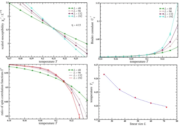
low-temperature regime spin correlation length and antiferromagnetic susceptibility are well described by renormalisation group; in high-temperature regime a ﬁt to BKT behaviour is much more accurate. The latter indicates a certain similarity with BKT transition. Their conclusion relies on the study of spin correlation length ξ, susceptibility χ(q0)

and spin stiﬀness. ξ is estimated with Orstein-Zernicke relation:

χ(q) = 1 L2 X i,j hSi· Sji T e iq(Ri−Rj) = χ(q0) 1 + ξ2_{(q − q} 0)2 (2.7) The temperature T∗ _{of this sharp crossover is compatible with Miyashita’s and}

Kawa-mura’s results who found with quite a simple Monte Carlo approach T ≈ 0.3 as a transition temperature. Contrary to above cited authors who consider it merely as a sharp crossover, Kawamura supports the idea of a peculiar transition. The original ar-gument by Kawamura and Miyashita [50] is based on a thorough discussion of vortices in HTAF. As said these are Z2 vortices and not Z vortices as is the case in XY systems

that exhibit BKT transition. To track the behaviour of vortices they introduce a vor-ticity function that is defined on the dual lattice links: 120-degree structure now stands at a vextex of the dual lattice; on the oriented links in the dual lattice the rotation of 120-degree structures from one end of the link to the other is a well-defined object that can be represented by an SU(2) matrix U. Vorticity V is the function defined on closed loops C as follows: V(C) = 1 2tr Y i∈C Ui ! (2.8) They showed that vorticity undergoes a transition between a perimeter-law asymptotic behaviour at low-temperature (T < T∗_{) and an area-law asymptotic behaviour at high}

temperature (T > T∗_{), which is similar to the behaviour of Wilson’s loops [131, 55]:} VR = hV (CR)i −→

R→∞

®

exp(−αA) T > T∗

exp(−βR) T < T∗ (2.9)

where CR is a loop of length R, A is the enclosed area. In fact this point emphasises

(26)

2.2. BRIEF REVIEW OF ZERO-FIELD BEHAVIOUR 17

high-temperature phase. On this particular point all groups do agree. On the nature of the change at T∗ _{there is a disagreement. Kawamura and coworkers further support}

their viewpoint [53] pointing out the existence of two different length scales. Indeed as already discussed in their early paper [51, 50], the transition cannot be a BKT one. It is then hardly surprising that they disagree with other groups like Wintel and his coworkers who are specifically looking for a BKT transition. Let’s further develop the argument. Vorticity exhibits a sharp drop from low-temperature regime to high-temperature regime, similarly to what happens in a usual BKT transition. There is however an important difference: in HTAF spin stiffness doesn’t undergo any such sharp drop whereas in usual BKT transition both spin stiffness and vorticity behave the same way with a jump at the same temperature. Here comes the main difference between a BKT transition and what occurs in HTAF: the existence of two different length scales, namely the one of spinwaves and the one of vortices [53]. The former doesn’t diverge at the transition contrary to the latter. In other terms the system is characterised by two different stiffnesses. Spin correlation function C(rij) = hSi· Sji can be factorised into

a spinwave contribution and a vortex contribution, the same way it is done for BKT transitions: C(rij) = Csw(rij)Cv(rij) [40]. Assuming the normal exponential form for

correlation functions, correlation length then reads:

ξ= ξswξv

ξsw+ ξv

(2.10) Consequently in the vicinity of the transition where ξv ≫ ξsw correlation length exhibits

a weak essential singularity:

ξ ∼ ξsw Ç 1 −ξsw ξv å (2.11) Spin correlation length remains ﬁnite at low temperature: spin correlation decays expo-nentially both above and below the transition. This exponential decay was expected due to Mermin-Wagner theorem; a more sophisticated argument based on topological con-siderations consists in the following: symmetries involved in a phase transition can be found and analysed through the space associated with low-temperature phase removing its topological defects, here vortices, and retaining all other parameters equal. In topo-logical language this means calculating the universal covering of the order parameter space. Here the universal covering of SO(3) is S3_{, the three-dimensional sphere. S}3

is the order parameter space of Heisenberg ferromagnetic four-component spin system as well: in two dimensions, spin correlations in this system decay exponentially, which indicates the same occurs in HTAF at zero ﬁeld. Low-temperature phase is not an ordered state in the traditional way but is topologically ordered as the single accessi-ble sector is the one without any free vortex. The nature of low-temperature phase is thus rather uncommon: Kawamura and coworkers proposed to call such a state that is neither a liquid nor an ordered AF state a spin gel [53].

(27)

2.3 Finite-field behaviour: symmetry discussion

As discussed in the preceding section, zero-field behaviour excludes finite-temperature transition to a long-range ordered phase with a gapped spectrum, ie a massive phase. It was consequently quite surprising to realise so far published phase diagrams depict transition lines going to a finite-temperature multicritical point at zero-field [52], which disregards an essential feature of HTAF, namely that zero-field configurations are mass-less. Indeed the existence of such a multicritical point would imply an infinitesimally small field makes the system massive: this is quite questionable a statement! For this reason it was necessary to examine anew finite-field behaviour in Heisenberg triangular antiferromagnet. A more natural viewpoint is indeed that finite-field transition lines close at (T, h) = (0, 0).

Looking back at the antiferromagnetic order parameter in Eq. (2.6) symmetries at ﬁnite ﬁeld can be discussed. If we consider a simple translation ˆTa with a lattice vector

a (ri → ri+ a) the order parameter is transformed as

ˆ

Ta[l1+ il2] = (l1+ il2)e−iq0·a (2.12)

with the phase factor q0 · a ∈ {0, ±2π/3}, which means that an inherent discrete Z3

symmetry exists besides the continuous S1 _{symmetry associated with free rotations}

about the direction of the applied ﬁeld ˆz. Hence the system is governed by a compound symmetry S1 _{⊗ Z}

3. Yet as seen with (2.5) a continuous degeneracy still exists: it

doesn’t match any symmetry in the Hamiltonian. In such a case it is legitimate to wonder whether this degeneracy of ground state manifold is robust against fluctuations. For a degeneracy not associated with any symmetry of the Hamiltonian, no Goldstone mode exists [34], which implies there is no entropy gain for such states. In our case relevant fluctuations are thermal ones. As shown by Sheng and Henley [106], thermal fluctuations must be calculated at higher order than the second one for degeneracy to be removed; a selection does occur reducing degeneracy to S1_{⊗ Z}

3. This reduction of

degeneracy is an example of an ‘order by disorder’ scheme [124].

At low temperature and low field the expected stable configuration is the so-called 120-degree configuration which is a natural solution of (2.5). A simple calculation shows that 120-degree configuration is not stable above h = 3. Since ground state configurations are defined by the configuration on any triangle, let’s write (2.3) using a three-sublattice pattern:

H = N_{3 ×} 1_{2 ×}6 (m1· m2+ m2· m3+ m3· m1) −

N

3 h (m1 + m2+ m3) = Nε

where mi = hSii is thermal averaged value of the spins of i−th sublattice, N is the

number of spins, and ε the average energy per spin:

ε= m1· m2+ m2· m3+ m3· m1−

h

(28)

2.3. FINITE-FIELD BEHAVIOUR: SYMMETRY DISCUSSION 19

θ

Figure 2.1: Distorted 120-degree structure with the definition of the angle θ. The structure is rotationally symmetric about the dashed axis that stands for the external field direction or the anisotropy axis (as discussed in Sec. 3.1). The three arrows stand for the three spins of a triangular plaquette.

The energy of a deformed 120-degree structure (see Fig. 2.1) then reads:

ε = cos 2θ − 2 cos θ +h

3(1 − 2 cos θ) (2.14)

The minimisation of (2.14) with respect to θ yields: cos θ = 1 2 Ç 1 + h 3 å (2.15) which shows such a conﬁguration exists if and only if h 6 3.

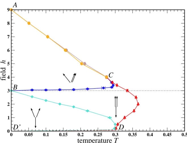
At T = 0 a transition must therefore occur between low-field (h < 3) and high-field (h > 3) regimes. In fact an intermediate phase separates the low-field low-temperature and quasi long-range ordered 120-degree phase from high-field configuration [35]. The intermediate phase corresponds to one-third magnetisation plateau: it is an up-up-down collinear configuration. Consequently spin-flop transition doesn’t exist: instead double continuous transitions occur. At T = 0, this intermediate collinear phase is confined to the point h = 3 that hence is a critical point that can be studied in quantum limit as an interesting quantum critical point. At finite temperature, thermal fluctuations are strong enough to stabilise this collinear phase in a larger domain of temperature-field plane in low field region (high fields obviously suppress up-up-down structure). At high field thermal fluctuations select a planar configuration instead of umbrella structure [106]: in this configuration two sublattices develop the same magnetisation [22] and non-zero transverse magnetisation exists as illustrated in Fig. 2.2.

(29)

β α

Figure 2.2: High-field planar structure that is stabilised at h > 3, referred to as V-shape configuration in the text. It is characterised by l2 = 0, l1 with components both along the

direction of the dashed line that is the direction of field and of the easy-axis in case of easy-axis HTAF, and transverse to this direction and m along the dashed line. The three arrows stand for the three spins of a triangular plaquette.

The natural question is then the nature of phase transitions occurring in the system. Such a treatment can be carried out discussing the order parameter symmetries. Con-sidering the order parameter space, S1_⊗Z

3, a discrete and a continuous symmetry have

to be broken. Diﬀerent scenarios are possible as Korshunov discussed it [60, 57, 58, 59]. Naturally there are three of them: either (i) the restoration of S1 _{occurs before the}

restoration of the discrete symmetry or (ii) it is the opposite way round or (iii) there is a single transition that belongs to a new universality class. The latter case seems quite exotic and rather unlikely: the reason why it may have been suggested in some numerical studies is that numerical accuracy at that time was too limited to distin-guish both transitions. Modern numerical investigations have ruled it out. First two scenarios involve excitations associated with each symmetry: vortices for the continuous symmetry, domain walls for the discrete symmetry. As a consequence it is possible to investigate the restoration of the compound symmetry analysing the behaviour of these excitations, or in other words tools used to investigate each transition can be used (spin stiﬀness and/or vorticity for S1_{, correlation function and/or susceptibilities for Z}

3). A

major diﬀerence between both scenarios is that in the second case fractional vortices form at kinks on domain walls [60, 57, 58], which implies the jump in spin stiﬀness is larger than it is in case of integer vortices, namely (2q2_/π_{)T for 1/q vortices. This can}

be considered a deﬁnitive way to distinguish between both scenarios.

To discuss the succession of phase transition it is necessary to distinguish low-field and high-field regions as the involved spin configurations are different. In low-field region, as previously mentioned, thermal fluctuations stabilise up-up-down collinear phase, which thus appear as an intermediate phase between 120-degree configuration and both high-field configuration and high-temperature (paramagnetic) phase. This means that discrete symmetry-breaking occurs first (in this case Z3) then

continu-ous symmetry-breaking (S1_{). Indeed collinear structure only breaks Z}

3 symmetry and

leaves S1 _{symmetry unbroken. The latter breaks down in 120-degree conﬁguration.}

(30)

dif-2.3. FINITE-FIELD BEHAVIOUR: SYMMETRY DISCUSSION 21

ferent: Z3 symmetry-breaking is associated with the component along ﬁeld direction

whereas S1 _{symmetry-breaking is associated with transverse component. As ordering}

occurs along different components in low-field region, the order of phase transition is clear and associated universality classes as well: the upper transition corresponds to the ordering along the field (up-up-down structure) and pertains to three-state clock model universality class (cf.[9]) whereas the lower transition corresponds to the ordering along a transverse direction (120-degree structure) and pertains to a BKT universality class. At high fields the situation is less clear because there is only one ordered phase which corresponds to a planar spin configuration with spins on two sublattices iden-tical and with a finite transverse magnetisation, so-called V-shape configuration (see Fig. 2.2). As l2 = 0 in this high-field configuration, there is a single order parameter

involved in the breaking of two symmetries. In real space the ordering actually occurs along a single component, namely the transverse one; the ordering of parallel compo-nent is induced by the ordering of transverse compocompo-nent as can be seen considering the following term of Landau-Ginzburg functional that comes into play: Sz

q Ä S⊥ q ä2 , which indicates that transverse component acts as an ordering ﬁeld on parallel component. As previously discussed the breaking of compound symmetry Z3 ⊗ S1 at once is quite

unlikely: successive transitions corresponding to the successive breaking of each com-ponent of this compound symmetry are thus expected. The tricky question to answer to is then the order of these transitions. Korshunov demonstrates case (ii) implies the existence of fractional vortices centered at kinks on domain walls. Numerically it can be checked examining spin stiﬀness jump at binding-unbinding transition: the jump for a 1/q fractional vortex is indeed (2q2_/π_)T

BKT. From this observation he draws

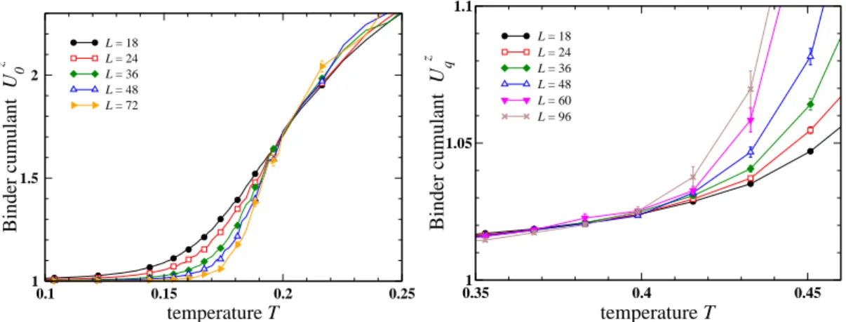
the conclusion that scenario (i) necessarily occurs: the transition temperature for the binding-unbinding transition of fractional vortices is indeed much lower than the es-timate for the transition associated with domain walls (percolation threshold), which is contradictory with scenario (ii). Consequently there is no fractional vortices and scenario (i) should occur. In next section a way to numerically ﬁnd out the transition sequence is proposed.

(31)

0 0.05 0.1 0.15 0.2 0.25 0.3 0.35 0.4 0.45 0.5

temperature T

0 1 2 3 4 5 6 7 8 9

field

h

B

C

A

D

D’

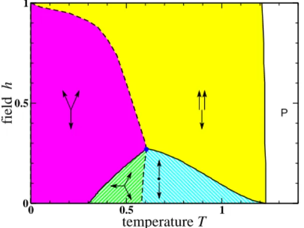
Figure 2.3: Phase diagram of Heisenberg triangular antiferromagnet. Solid lines are a guide to the eye linking calculated points. Dashed lines indicate theoretically expected transitions for which precise numerical results have not yet been obtained. Spin structures are sketched by the configuration on a triangular plaquette with z axis assumed vertical and xy plane perpendicular to the plane of the sheet.